Báo cáo hóa học: " Research Article Collaborative Area Monitoring Using Wireless Sensor Networks with Stationary and Mobile Nodes" docx

Hindawi Publishing Corporation
EURASIP Journal on Advances in Signal Processing
Volume 2009, Article ID 750657, 16 pages
doi:10.1155/2009/750657

Research Article
Collaborative Area Monitoring Using Wireless Sensor Networks
with Stationary and Mobile Nodes
Theofanis P. Lambrou and Christos G. Panayiotou
KIOS Research Center for Intelligent Systems and Networks, Department of Electrical and Computer Engineering,
University of Cyprus, Nicosia 1678, Cyprus
Correspondence should be addressed to Theofanis P. Lambrou,
Received 1 August 2008; Revised 10 December 2008; Accepted 4 March 2009
Recommended by Frank Ehlers
Monitoring a large area with stationary sensor networks requires a very large number of nodes which with current technology
implies a prohibitive cost. The motivation of this work is to develop an architecture where a set of mobile sensors will collaborate
with the stationary sensors in order to reliably detect and locate an event. The main idea of this collaborative architecture is
that the mobile sensors should sample the areas that are least covered (monitored) by the stationary sensors. Furthermore, when
stationary sensors have a “suspicion” that an event may have occurred, they report it to a mobile sensor that can move closer to the
suspected area and can confirm whether the event has occurred or not. An important component of the proposed architecture is
that the mobile nodes autonomously decide their path based on local information (their own beliefs and measurements as well as
information collected from the stationary sensors in a neighborhood around them). We believe that this approach is appropriate
in the context of wireless sensor networks since it is not feasible to have an accurate global view of the state of the environment.
Copyright © 2009 T. P. Lambrou and C. G. Panayiotou. This is an open access article distributed under the Creative Commons
Attribution License, which permits unrestricted use, distribution, and reproduction in any medium, provided the original work is
properly cited.

1. Introduction
Recent progress in two seemingly disparate research areas
namely, distributed robotics and low power embedded
systems has led to the creation of mobile sensor networks

[1]. Autonomous node mobility not only brings with it
its own challenges, but also alleviates some of the traditional problems associated with static sensor networks. It is
envisaged that in the near future, very large scale networks
consisting of both mobile and static nodes will be deployed
for applications ranging from environmental monitoring to
military applications [2].
In this paper we consider the problem of monitoring a
large area using wireless sensor networks (WSNs) in order to
detect and locate an event. In this context, we assume that the
event emits a signal that is propagated in the environment.
The sensors capture attenuated and noisy measurements of
the signal and the objective is to reliably detect the presence
of the event and estimate its position. By reliably we mean
that we would like to minimize the probability of miss event
(an event that remains undetected) subject to a constraint on

the probability of false alarms (the sensors report an event
due to noise). Note that in many applications false alarms
are as bad (if not worse than) as missed events. In addition
to the incurred cost for sending response personnel to the
area of the event, frequent false alarms may lead the users to
ignore all alarms, and as a result even detected events will go
unnoticed.
To achieve reliable detection in a large area, it is necessary
to deploy a huge number of sensors which with the current
technology implies a prohibitive cost [3]. For example,
consider a lake to be monitored for events (an event can be
a boat that spills a substance in the lake that changes the
water turbidity). If the lake has an area of 20 km × 20 km,
and we assume that each sensor has a reliable sensing range

(detection range) rd =10 m, then the number of sensor nodes
needed to monitor the entire lake is of the order of 106 which
with today’s technology implies a prohibitive cost.
Given that it is infeasible to reliably cover the entire
area with stationary nodes, in this paper we investigate
an alternative way of monitoring the area using several
stationary and some mobile sensor nodes that collaborate


2
in order to improve the area coverage and/or to detect an
event as fast as possible. The main idea is that the mobile
nodes will collaborate with the stationary nodes (and with
each other) in order to sample areas that are least covered by
the stationary nodes. In the context of WSNs, sensor nodes
are fairly inexpensive and unreliable devices, thus it is not
feasible to have an accurate state of each sensor node in the
field (some nodes may have failed or been carried away).
As a result one cannot have all necessary information to
centrally solve a path planning problem and predetermine
the path that each mobile sensor node should follow in
order to sample the areas least covered. In the proposed
approach, mobile nodes navigate through the sensor field
autonomously using only local information (i.e., the mobile
node’s beliefs and measurements as well as information
collected from the nodes, stationary or mobile, that are in
a neighborhood around the mobile).
This paper investigates the use of signal processing
techniques in the path planning of mobile agents for
improving the area monitoring in the context of WSNs. The

main contribution of this paper is that it investigates a family
of path planning algorithms and proposes a distributed
algorithm that is fairly simple; it relies only on local
information (i.e., information collected from the mobile’s
neighborhood) and can achieve very good performance. The
strategy used by each mobile is based on receding horizon
optimization and is motivated by the approach presented
in [4] where two or more agents are moving in an area
cooperatively searching for targets of interest and avoiding
obstacles or threats. At every step, the mobile node tries to
move toward, the least covered area, and at the same time it
avoids areas covered by other nodes. In the context of WSNs,
several approaches exist for identifying the point where a
mobile node should go in order to improve the area coverage
(for details see Section 6). All these approaches solve a static
problem and to the best of our knowledge, none of them
considers the path that the mobile node should follow in
order to get to its destination.
The paper is organized as follows. Section 2 describes
the model that has been adopted and the underlying
assumptions. Section 3 presents a family of distributed path
planning algorithms that can be utilized by each mobile
sensor in order to navigate through the sensor field. Section 4
presents the dynamic target estimation and allocation strategy used for coverage, event detection and collaboration
purposes. Section 5 presents several simulation results using
various sensor fields with randomly deployed sensor nodes.
Section 6 reviews related work in two research fields, the area
coverage for both stationary and mobile sensor networks and
the path planning algorithms in the fields of mobile robotics
and unmanned aerial vehicles. The paper concludes with

Section 7.

2. Model Description and Problem Formulation
2.1. The Environment. The environment is represented as
a rectangular area A = Rx × R y . We consider a set S
with S = |S | static sensor nodes that are randomly placed
in the area A, at positions xi = (xi , yi ), i = 1, . . . , S. In

EURASIP Journal on Advances in Signal Processing
addition, we assume that a set M of M = |M| mobile
sensor nodes are available and their position after the kth
time step is xi (k) = (xi (k), yi (k)), i = 1, . . . , M, k = 0, 1, . . ..
For notational convenience, we define the set of all sensor
nodes N = S ∪ M and reindex all mobile nodes as m =
S + 1, . . . , S + M. It is assumed that all sensors know their
location through a combination of GPS and localization
algorithms. Furthermore, it is assumed that all sensors can
reach the fusion center (commonly referred to as sink in the
WSN literature) using multihop communication.
In addition, we consider a set E with E = |E | stationary
nonoverlapping event sources (sources with nonoverlapping
footprints.) that are randomly placed in the environment at
positions e j = (xe , y e ), j = 1, . . . , E.
j
j
Next, we also define the neighborhood of a sensor s
as the set of all sensors that are located at a distance less
than or equal to rc from the mobile. In other words, the
neighborhood of sensor s ∈ N is the set of all sensors that
are in the disc centered at xs with radius rc :

Hrc (s) = j : xs − x j ≤ rc , j ∈ N , j = s
/

(1)

for all s = 1, . . . , S + M. If rc is the communication range of
the sensor, then Hrc (s) defines all sensors that are one hop
away from that node. In general however, one can define
larger neighborhoods that include sensors that are two or
more hops away.
2.2. Sensor Model. We assume that each event source j ∈ E
emits a constant signal V j in the surrounding environment.
As we move away from the source, the measured signal is
inversely proportional to the distance from the source raised
to some power α ∈ R+ which depends on the environment.
As a result, the tth measurement of sensor i ∈ N is given by
⎧
⎨

⎫

Vj ⎬
zi,t = min⎩Vsat ,
+ wi,t ,
rα ⎭
j =1 i j
E

(2)

where Vsat is the maximum measurement which can be
recorded by a sensor, ri j is the radial distance of sensor i from
the event source j,
ri j =

xi − x e
j

2

2

+ yi − y e ,
j

(3)

and wi,t is additive Gaussian noise with zero mean and
variance σi2 . A sensor node reports that it has reliably
detected an event if the measurement it receives is greater
than the detection threshold τd (Alternatively one could use
the average measurement or simply assume smaller noise
variance.) . This threshold is determined in a way such that
the probability of false alarm is less than a given constraint
p f a . This calculation can be done as in [3] and references
therein, but for the purposes of this paper, it is assumed
that this threshold is given. This threshold together with V j
defines a disc around the source (footprint of the source)
where, if sensor i is located inside this disc, then it will be
alarmed (i.e., its measurement will be above the threshold τd )

EURASIP Journal on Advances in Signal Processing

3

with high probability, at least 0.5. Given the model (2), the
radius of the disc is given by
rd =

α

Vj
.
τd

(4)

By symmetry, there exists a disc around every sensor with
radius rd where if a source exists it will cause the sensor
to be alarmed with high probability (at least 0.5). This is
referred to as the detection (sensing) range of the sensor and
it is assumed known. For the purposes of this paper, if the
event occurs within this disc, then we say that it is reliably
detected. Furthermore, we assume that an event is detected
by the network if at least one sensor (stationary or mobile)
detects the event but other fusion rules can also be used at
the fusion center.
Similarly, we assume that we are given a “suspicion”
threshold τs < τd such that if the measurement of the sensor

i, τs ≤ zi ≤ τd , then sensor i does not report a detection,
however, it may report that it “suspects” that there may be
an event around its area. Note that τs defines a disc around
the sensor with radius rs > rd , and thus a node may report
the suspicion if the event exists in the “donut” that is formed
by the suspicion disc when the detection disc is removed.
The event suspicion may be used in different ways. It can be
reported to the sink which may fuse the information from
several sensors or it can be given to a nearby mobile node
which will collaborate with the stationary sensors in order
to move closer to the suspected event area to confirm the
existence or not of the event. In this paper, the suspicion will
be used as in the latter example.
2.3. Objectives. The aim of this paper is to plan the path
of the mobile nodes in order to achieve certain objectives.
As already mentioned, the sensor network environment is
constantly changing (sensors may fail or be carried away)
thus it is unrealistic to expect that a central controller will
have all necessary information to predetermine the paths
that each mobile should follow, and thus we will consider
dynamic path planning algorithms that use locally available
information to determine where to go next.
In this type of problems, one can define different
objectives that may result in different strategies. A possible
objective is to detect and locate events as fast as possible. For
this objective, a candidate strategy for the mobile nodes is
to quickly move toward large uncovered areas since, if there
exists an undetected event source, it is most likely located
in those areas. Another possible objective is to maximize the
area coverage (minimize the average probability that an event

source remains undetected). In this case, a good candidate
strategy for the mobile is to navigate through areas not
covered by other sensors (stationary or mobile). As will be
shown in the sequel, it turns out that a combination of these
two strategies can achieve very good results.
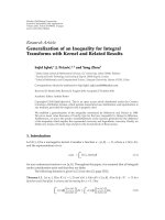
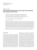
To make the concept of area coverage more concrete,
we divide the field area in small squares with side da. In
other words, we transform the sensor field area A into a grid
G of size X × Y , where X = Rx /da and Y = R y /da
(see Figure 1). Thus, we assume that any sensor s ∈ N is

Stationary sensor

Suspicion range rs

Mobile sensor

Event

Detection range rd

Coverage hole center

Figure 1: Environment Model.

located in the cell zs = (i, j), i = xs /da and j = ys /da
(i.e., zs is the discretized coordinate corresponding to xs ).
Furthermore, we assume that a sensor located in the cell zs ,
depending on the detection range d = rd /da , covers a
neighborhood of cells D d (zs ):

D d (zs ) =

p, q : p − i

2

+ q− j

2

2
≤ ld , zs = i, j

.
(5)

We associate with the grid G, an X × Y matrix Gk , k = 0, 1, . . .,
where each element of Gk captures our “confidence” that if
an event occurs in the corresponding area of the field, it will
be detected by the sensor network. If the (i, j)th cell falls in
the detection range of a static sensor, then the corresponding
Gk (i, j) = 1, for all k (here we use the fact that a stationary
sensor may perform a long run average of its measurements
and thus the probability of detecting a source in its detection
range goes to 1). Otherwise, initially (at k = 0) Gk (i, j) =
0 and as the mobile nodes move around, if they sample
areas not covered by the static sensors, then our confidence
increases and continues to increase as the mobiles take more
samples. Furthermore, if a cell has not been sampled for
some time, then it is possible that our confidence will be

reduced. Thus at every step, we use the following updating
rule for every element of matrix Gk :
⎧
⎨0.5 · Gk i, j +0.5,

Gk+1 i, j = ⎩
f · Gk i, j ,

if i, j ∈ D d (zs ), s ∈ N ,
otherwise,
(6)

where 0 ≤ f ≤ 1 is the “forgetting” factor. This factor can be
used to account for the physics involved with the phenomena
of the events that are being monitored. For example, it can
account for sources that are active only during a window
of time of the observation interval or sources that turn on


4

EURASIP Journal on Advances in Signal Processing
y1

and off at various time instances. Consequently, coverage is
defined as
Ck =

1
X ×Y

×

Gk i, j .

yi

(7)

1≤i≤X
1≤ j ≤Y

2.4. Mobile Sensor Node Model. The state of the ith mobile
node at time k is denoted by υi (k) which is comprised
of two components, υi (k) = [xi (k), θi (k)]. As already
mentioned xi (k) is the node’s position and θi (k) is its
orientation (heading direction). The mobile nodes move at
some constant speed ψ and make path planning decisions at
discrete time intervals, which means that each mobile node
follows a straight line of length ρ = xi (k + 1) − xi (k) when
moving from xi (k) to xi (k + 1). Moreover, we point out that
this model can also include maneuverability constraints of
the mobile platform using some angle φ which constrains the
maximum allowed difference between θi (k) and θi (k + 1).
Finally, we describe the information required by each
mobile in order to make path planning decisions. Each
m
mobile uses a coverage cognitive map, an X × Y matrix Pk ,
m
m ∈ M where it keeps the state of the field. Ideally Pk should

m
remain Pk = Gk at all times k, since the matrix Gk represents
the accurate global state of the field which is used for the
computation of the field coverage Ck . Clearly, in a dynamic
environment where several sensors may accidentally move,
fail or more sensors are added, it is impossible to guarantee
m
that Pk = Gk at all times. However, we emphasize, that
the proposed algorithm, that will run by a mobile located
at some zm (k), computes its next position based mainly on
m
local information, that is, information in the submatrix of Pk
that corresponds to the cells D c (zm (k)), where c = rc /da
and thus, it is sufficient to have accurate information only
for the D c (zm (k)) submatrix. This is easily attainable since
the required information can be obtained from the mobile’s
neighbors in Hrc (m).

3. Collaborative—Distributed Path Planning
In this section we present a family of distributed path
planning algorithms that can be utilized by each mobile
sensor in order to navigate through the sensor field and
to achieve its objectives. These algorithms are based on a
receding-horizon approach and are motivated by [4]. In this
family of algorithms, the mobile’s controller evaluates the
cost of moving to a finite set of candidate positions and
moves to the one that minimizes the overall cost as described
next. Before we proceed, to simplify the notation, in this
section, we dropped the index for each mobile, that is, x(k)
refers to the position of the ith mobile sensor, i ∈ M.

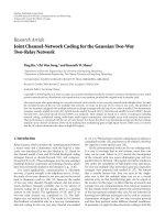
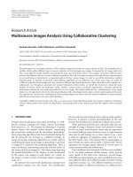
Suppose that during the kth step, the mobile node is
at position x(k) and it is heading to a direction θ. The
next candidate positions are the ν points y1 , . . . , yν that are
uniformly distributed on the arc that is ρ meters away from
x(k) and are within an angle θ − φ and θ + φ as shown
in Figure 2. Note that the parameters ρ and φ can be used
to also model the maneuverability constraints of the mobile
platform. At the kth position, the mobile node evaluates a

yν
φ
x(k)

ρ

θ

Figure 2: Evaluation of the mobile node’s next step.

cost function J(yi ) for all candidate locations (y1 , . . . , yν ) and
moves to the location x(k +1) = yi∗ where i∗ is the index that
minimizes J(yi ):
J yi∗ = min J yi .
1≤i≤ν

(8)

The cost function J(·) is of the form
J yi =

w j J j yi ,

(9)

j ∈F

where F is a set of indeces such that the functions J j , j ∈
F are normalized cost functions with 0 ≤ J j ≤ 1 and
are defined to achieve certain objectives. For the purposes
of this paper, F = {t, c, s, r, m, b} but other functions can
also be included. The objective of Jc and Js is to achieve
collaboration between the mobile and its neighboring nodes
that are very close to it using only local information. On
the other hand, the objective of Jr and Jt is to use more
“global” information in order to avoid local minima. Jm is
a function for achieving collaboration between two or more
mobile nodes and finally Jb is a function for avoiding getting
out of the area boundaries. Furthermore, w j , j ∈ F are
positive weights that tradeoff the various objectives (e.g.,
if it is desired that a mobile moves quickly to its target
destination, then wt is made large).
3.1. Path Cost Functions. In this section we present the details
for the cost functions that we found to give the best performance among the algorithms that we have investigated. For
completeness, other functions that have been investigated are
placed in an appendix.
3.1.1. Neighboring Sensor Collaboration Cost Function Using
an Artificial Function. A main objective of the collaboration
between the mobile and stationary nodes is for the mobile
to avoid areas that have been covered by other nodes. The
objective of this function is to push the mobile away from

areas covered by other sensors. The cost function Js (y) used


EURASIP Journal on Advances in Signal Processing

5

involves a repulsion force that pushes the mobile away from
its closest neighbor. The form of this function is given by
⎧
⎪
⎨

⎛
⎜

Js y = max ⎪exp⎝−
j ∈Hrc (m)⎩

y − xj
2
rd

2⎞

⎫
⎪
⎬

⎟

⎠⎪,
⎭

(10)

where Hrc (m) is the set of all nodes in the communication
range of the mobile m. The detection range rd quantifies
the region size around the mobile m to be repelled by its
neighbors. A related function that we considered consists of
the total force applied to the mobile, that is, the resultant of
all repulsion forces from all neighbors. However, we found
that its performance was inferior to that of (10) and thus we
do not consider it any further in the paper.
3.1.2. Target Cost Function. Assuming that the mobile has a
target destination point xt , the cost Jt (y) is a function that
pulls the mobile toward its target and is a function of the
distance between the mobile and the target position. This
function should take a smaller value as the mobile moves
toward the target destination and thus for the purposes of
this paper it is given by
Jt y =

y − xt

,

(11)

where is the maximum distance between the mobile node
and its target and is used for normalization purposes. There

are several ways that one can use to assign a target position
to a mobile. For example, target points may be chosen by
a central controller as part of the mobile’s mission. During
a subsequent section we will describe alternative ways of
determining the target position for each mobile. Depending
on the mode of the mobile’s movement, its target may be
either an area that is poorly covered (monitored) or the
estimated location of a “suspected” source.
All cost functions used in the paper can be easily computed by a mobile node using information in its cognitive
map or by obtaining information from its neighbors. To
compute Jt (·), one needs to determine a target position (xt )
and this will be done in the next section.

4. Dynamic Target Estimation and Allocation
In addition to the possibility of prespecifying a target
position for the mobile, in this paper we investigate the
possibility allowing the mobile to dynamically determine its
target position xt ; at every step k the mobile uses the collected
information to determine its new target location. We point
out that it is even possible for a mobile to have two target
positions, a short term as well as a longer term target (i.e.,
include two similar terms in (9) with different weights).
The dynamic target estimation is performed using two
different algorithms depending on the state of the measurements obtained by the mobile and its neighbors as shown in
Figure 3. If the mobile does not get any “suspicion” messages
from its neighbors (i.e., all obtained measurements are below
the suspicion threshold τs ), then the mobile is in a coverage

mode and its target is the biggest coverage hole in some
neighborhood around the mobile (the size and shape of this

area can be a parameter of this problem). On the other hand,
if the mobile receives at least a “suspicion” message then
it goes into the search mode and the target becomes the
estimated event source position. Finally, if an event source
is detected by the mobile, we assume that it is neutralized
and that the mobile moves towards its next target (This is a
modeling assumption that may not be very practical. On one
hand we may assume that the actual time between the step
that the mobile detected the event and the next one is long
enough to allow a response crew to respond. On the other
hand, the mobile may be programmed to ignore (subtract)
the signal from the known sources so it can continue its
mission.) . Next we present the specific algorithms used in
each case.
4.1. Coverage Hole Estimation Scheme—Zoom Algorithm.
In this subsection we present a computationally efficient
algorithm for coverage hole detection. Using the coverage
hole detection algorithm a central controller (e.g., the sink)
can estimate the coordinates of up to the M biggest coverage
hole centers (which can become the target coordinates of the
M mobiles). In other words, the aim of this algorithm is to
determine where the M mobiles should be placed in order
to maximize coverage (i.e., maximize (7)). We emphasize
that this algorithm can run either by any central controller
on the entire field to obtain up to M coverage holes, or by
each mobile node itself, to estimate the coordinates of the
biggest coverage hole center inside a neighborhood rc at each
moving step k. Since this algorithm may run frequently (as
new information regarding the state of the field becomes
available) it is required that it is computationally efficient.

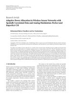
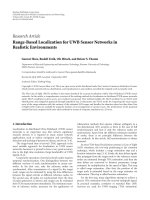
Using the principle of divide and conquer we propose the
Zoom Algorithm which is very efficient in computation complexity, time and memory. The idea is to divide the grid (i.e.,
m
the matrix Gk ) or any subgrid (i.e., a submatrix of Pk that
corresponds to the cells D c (zm (k))) in four equal segments,
and choose the segment with the maximum number of
empty cells, that is, the segment with the maximum number
of cells with G(i, j) = 0. (Alternatively, one can choose the
segment with the least coverage as defined by (7)). Then, this
procedure is repeated either until the segment size is equal
to a single cell or until all segments have the same number
of empty cells. In the first case, the hole center position
will be the center of the cell. In the second case, the hole
center position will be the lower right corner of the upper
left segment (the center of the segment during the previous
iteration). Figure 4 illustrates the idea of zooming for hole
detection when this algorithm is used by each mobile node
in a distributed fashion. The details of the algorithm, when it
is used by a central controller, are listed in Algorithm 1.
More information and comparative theoretical and simulation results between the zoom algorithm and other ways
of finding the coverage holes can be found in [5].
4.2. Source Position Estimation Scheme. As mentioned earlier,
as each mobile node m navigates in the field, it continuously


6

EURASIP Journal on Advances in Signal Processing
τs < zi (k) < τd

zi (k) > τd

Target =
estimated
source
position

Target =
coverage
hole
position
zi (k) < τs

Source
detection

τs < zi (k) < τd
zi (k) < τs

Figure 3: The target allocation strategy for the ith mobile sensor node during the kth step.

Non updated
grid region
Updated
grid region

Static
sensor

Mobile sensor

communication
range

2

1

421

422
42

41

42 4

423
4

3

Coverage
hole position
(target)

44

43

(a)

Root

q1

q41

q 42 1

q4

q3

q2

q 42 2

q44

q43

q42

q 42 3

q 42 4

(b)

Figure 4: Illustration of the zoom algorithm (a) Grid segmentation (b) Generated tree.

EURASIP Journal on Advances in Signal Processing

7
is assumed that it is neutralized and the mobile resumes its
coverage function.

Zoom Algorithm
1: Import coverage cognitive map G
/∗∀i, j ∈ X, Y ⇒ c(i, j) = G(i, j)∗/
2:
C=G
3: for each mobile sensor m ∈ M
4:
for each zooming step zx , x = 1, . . . , κ
5:
for each segment qs , s = 1, . . . , 4 ∈ Zx
/∗ each segment has L/2zx × L/2zx cells ∗/
6:
for each cell (i, j) ∈ Qs
7:
if c(i, j) == 0
8:
a(qs ) = a(qs ) + 1
9:
end
10:
end
11:
end

12:
if a(q1 ) == a(q2 ) == a(q3 ) == a(q4 )
13:
xm = max{i : (i, j) ∈ Q1 )}
14:
ym = min{ j : (i, j) ∈ Q1 )}
15:
break
16:
end
∗
17:
(qs ) = arg max a(qs )
/∗ select next region to segment ∗/
∗
18:
xm = min{i : (i, j) ∈ Qs }
∗
19:
ym = min{ j : (i, j) ∈ Qs }
20:
end
21:
place mobile sensor at (xm , ym )
22:
for each cell (p, q) ∈ Nr (xm , ym )
23:
c(p, q) = c(p, q) + 1
24:
end

25: end

4.3. Distributed Target Allocation. The previous two subsections describe two different methods that can be used by
the mobiles in order to autonomously decide their target
location. Both methods utilize information that can be
obtained by the mobile from its neighborhood. In the case
of the coverage hole estimation, the information is included
in a relevant submatrix of the cognitive map, while for the
source position estimation the relevant information is the
measurements of the neighboring nodes. A possible problem
arises when two or more mobiles are close to each other. In
this case, it is very likely that the information they will use to
estimate the target position will be the same and as a result
they will all estimate the same target location. Clearly, this is
not a good collaboration strategy since there is no benefit if
they all converge to the same point.
To avoid this problem we utilize the following two
protocols depending on the state of the mobile node (i.e.,
searching for a source or coverage).
If a mobile node m is in searching mode and also in
communication range with other mobiles, then it queries
its neighboring mobiles for their current position and their
target locations. Then, it computes the distance between its
t
own target and the target of the neighboring mobiles dm, j for
all neighboring mobiles j,
t
t
dm, j = xm (k) − xtj (k) .

Algorithm 1: Pseudocode for the Zoom Algorithm.

samples the environment and also queries its neighboring
nodes about their positions and their sensor measurements
z j , j ∈ Hrc (m). In the case when one or more sensor
readings are between the τs and τd thresholds, the mobile
node uses the measurements to estimate a likely position of
the source which will then become its target location. For this
estimation, a number of estimation algorithms can be used
(e.g., see [6–8]). For the purpose of this paper non linear
least squares estimation has been used. The event source
location (target position) xt = (xt , yt ) is the solution to the
minimization problem:
⎛

J=

⎜
⎝ zi −
i∈Ω(k)

⎞2

V
2

(xt − xi ) + yt − yi

⎟

⎠
2 α/2

,

(12)

where Ω(k) is a set of measurements that includes the
measurements of the mobile’s neighbors at the kth step
together with any measurements obtained by the mobile up
until step k. In this paper, a uniform diffusion model [8] has
been adopted and also the initial source concentration V is
assumed to be known. We point out however that extension
for the case where V is unknown is straightforward. As
long as the mobile continues to get “suspicion” signals, it
continues to search for the source by updating the estimated
source position. As before, once the source are detected, it

(13)

If this distance is greater than a threshold value then it
assumes that the two mobiles are heading toward different
t
targets and thus it continues normally. If dm, j is less than
the threshold value then it is very likely that the two mobiles
are heading toward the same suspected point and thus only
one should continue the search toward that target while the
other should switch to the coverage mode. This decision is
based on the distance of each mobile from its target. The
mobile that is closest to its target continues the search while

the other switches to the coverage mode. For the purposes of
this paper, the threshold distance used to decide whether two
mobiles are heading toward the same target is set to 2rd .
Now if a mobile node m is in the coverage mode
and is also in neighborhood of other mobiles, then, in
order to avoid going toward the same point, it queries the
other mobiles in its communication range for their current
locations and their target points. Once a mobile has received
the target points of all mobile neighbors, then it updates
its cognitive map and assumes that these target points
constitute covered areas. Then it proceeds normally with
the coverage hole estimation algorithm (Zoom Algorithm).
With this simple scheme, the mobiles avoid exploring the
same areas. This scheme has some important benefits. It is
distributed (no need for a central controller), it is simple, and
it utilizes only local information (the relevant information
in the submatrix D c (zm (k)), which corresponds to the
neighborhood rc of the cognitive map).
Finally, it is worthwhile to mention that when two
mobiles come into communication range, they can also


8
exchange their cognitive maps so that a mobile does not
explore areas already explored by other mobile nodes.

5. Simulation Results
In this section we present some simulation results with some
representative scenarios that show the movement of a set of
mobile nodes and also compare the performance of different

path planning algorithms (all from the family of algorithms
presented in Section 3). Depending on which cost functions
are used in (9) and the weights, one can obtain different
algorithms. To distinguish between the different algorithms
investigated, we use acronyms where each letter corresponds
to the individual cost functions used, for example, TS refers
to an algorithm for which wt > 0 and ws > 0 while wc =
wr = wm = 0. (For all algorithms and all experiments to
prevent any mobile from going outside the area we have used
wb = 1).
Unless otherwise stated, all experiments refer to a square
300 m × 300 m field, and a grid with da = 1 m is used. The
mobile maneuverability parameters are set to ρ = 2 m and
φ = 30◦ while for every decision ν = 10 candidate next
positions are considered. For the event propagation model,
we assume that V = 1500, Vsat = 100, and the exponent
α = 2. Finally we assume that a detection threshold τd = 15,
and thus the sensing radius of all sensors (stationary and
mobile) is rd = 10 m and the communication radius rc =
4.5 · rd = 45 m (for the neighborhood of each sensor we only
consider its one hop neighbors).
Next we present some representative scenarios and show
the movement of a team of robots that uses the Distributed
TS algorithm, a simple algorithm that performed very well
against all other algorithms investigated. In this algorithm,
every mobile makes autonomous decisions using only the Jt
(with = rc ) and Js cost functions (i.e., wt = 0.8, ws = 0.2,
and wc = wr = wm = 0). For estimating the target positions,
the mobile uses either the coverage hole detection algorithm
(in coverage mode) or the source position estimation algorithm (in search mode) and the distributed target estimation

scheme presented in the previous section. Finally, for the
coverage hole detection algorithm only the cells in D c (zm (k))
are used. In other words, the coverage hole is estimated only
in its neighborhood.
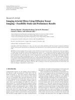
In the first simulation experiment we use a team of two
mobile nodes and show the behavior of the Distributed TS
algorithm in a field with 100 randomly deployed stationary
sensors. In this simulation scenario there is no event source
thus Figure 5 shows how the two mobile nodes navigate
collaboratively through the field, sampling points that are
not adequately covered by the stationary sensors. As seen
from the paths followed, there is collaboration between
mobile and stationary sensors in the sense that the mobiles
have found two different paths that are least covered by
the stationary sensors. Also notice how the two mobiles
collaborate and select different targets at the beginning
of their motion. Moreover note that one can adjust the
mobile’s parameters in order achieve different objectives. For
example, Figure 5(a) shows a path where the mobiles move
quickly through the field to achieve faster detection. On the

EURASIP Journal on Advances in Signal Processing
300
rc
250

200

150

Target
(coverage
hole center)

100

50

0

0

50

100

150

200

250

300

(a) Paths followed when the mobile’s objective is fast detection (wt =
0.8, ws = 0.2, rc = 45 m)
300
rc
250

200

150

100

50

0

0

50

100

150

200

250

300

(b) Paths followed when the mobile’s objective is better coverage
(wt = 0.2, ws = 0.8, rc = 25 m)

Figure 5: Dynamic path planning using a team of two mobile
nodes.

other hand, Figure 5(b) shows a scenario where the mobiles
try to achieve better coverage by covering a hole before they
proceed. Finally, we point out that given enough time, all
algorithms will cover the entire field.
Figure 6 shows the paths followed by two mobile nodes
when a set of five nonoverlapping static sources exist (each
source is turned on at the beginning of the simulation time
and stays on for the entire simulation with V = 3000).
We assume 100 randomly deployed sensors in the field. The
detection threshold of all sensors is τd = 30 (thus rd =
10 m), and the suspicion threshold is τs = 5 (rs = 24.5 m).
Figure 6 also shows the positions of the event sources. One
source is reliably detected by the stationary sensors however
for the remaining four there are no stationary sensors in
a radius rd around the event, and thus these events would
have remained undetected. Initially, both mobile nodes are


EURASIP Journal on Advances in Signal Processing

9

300

300

Coverage
hole center

250

250

200
200

rc
150

Source
position
estimates

150

rs
rd

100

100

Event
source

50

50

0

0

100

200

300

(a) Paths followed in an empty sensor field (0 stationary sensors)
0

0

50

100

150

200

250

300

Figure 6: Dynamic distributed path planning using a team of two
mobile nodes in the presence of event sources.

navigating towards their current estimated coverage hole

positions. Note that in some cases there are sensors within
rs from the event sources and these sensors are likely to
report the “suspicion” to the passing mobile node. Once a
mobile node gets a suspicion message from a static node in its
communication range (or its sensor measurement is inside
the “suspicion” region, τs ≤ zi ≤ τd ), then it switches its
target to the estimated location of the event.
The next simulation experiment demonstrates the behavior of the Distributed TS algorithm (with fixed parameters
as described above) for sensors fields with different densities
(empty, sparse and dense fields). Figure 7 shows the paths
followed by three mobile nodes after 300 moving steps. From
the figure it is evident that the Distributed TS algorithm is
able to easily adapt to different sensor node densities without
getting trapped in local minima. Mobile nodes always keep
navigating in the sensor field, passing/sampling through
uncovered regions and improving coverage. Figure 7(a)
shows that in the case of an empty field (no stationary
sensors are available) mobile nodes collaborate and navigate
similarly to standard search algorithms.
In the next simulation experiment (Figure 8) we investigate the value for the suspicion threshold τs . Note that there
exists a tradeoff in its actual value. If this threshold is set too
high, then the mobile will get in the searching mode rarely
(clearly τs < τd ). On the other hand, if this threshold is
set too low, then the mobile will be running after frequent
false alarms. In this experiment we evaluate the number of
detected sources over 20 sensor fields with 100 stationary
sensors. In each field 15 nonoverlapping event sources are
randomly placed. As shown in Figure 8(a) only a small
number of the sources is detected by the stationary sensors
(at time zero, about 6.5 sources on average are detected).

A group of two mobile sensor nodes using the Distributed
TS algorithm is employed. We measure the average number
of detected event sources as well as the average coverage

300
250

200

150

100

50
0

0

100

200

300

(b) Paths followed in a sparse sensor field (100 stationary
sensors)
300

250
200

150
100
50
0

0

100

200

300

(c) Paths followed in a dense sensor field (300 stationary
sensors)

Figure 7: Paths followed after 300 moving steps by a set of three
mobile sensor nodes using the distributed path planning algorithm
for different sensor field densities.


10

EURASIP Journal on Advances in Signal Processing

Number of event sources found

13

(1) RCM. This algorithm has been developed in [4, 9]

for cooperative search missions by UAVs. The RCM
algorithm uses the cost functions Jr , Jc , and Jm with
the following weights wr = 0.5, wc = 0.2, wm = 0.3
and with triangle parameters δ = 15◦ and μ = 40.
Note that since this algorithm does not use the Jt
function, it can only navigate in the field to reduce
uncertainty (maximize coverage) and cannot move
towards a target.

12
11
10
9
8
7
0

100 200 300 400 500 600 700 800 900 1000
Time steps
τs = 1
τs = 5
τs = 10

τs = 12
τs = 15

(a) Average number of nonoverlapping event sources found over 20
sensor fields

(3) TSM. This algorithm is similar to the TCM algorithm

(uses a central controller to solve the global target
assignment problem). The TSM algorithm uses the
following cost functions Jt , Js , and, Jm with the
following weights wt = 0.5, ws = 0.2, and wm = 0.3
√
and with parameters = 2A, where A is the sensor
field area.

80

70
Coverage

(2) TCM. In this algorithm a central controller decides
the next step of each mobile node. Once a mobile
node approaches its target destination a new target
(coverage hole point) is assign to the mobile using
a centralized target assignment scheme where the
controller computes the biggest coverage hole in the
entire field which is not already assigned to other
mobile nodes. The TCM algorithm uses the following
cost functions Jt , Jc , and Jm with the following weights
wt = 0.5, wc = 0.2, wm = 0.3 and with parameters
√
= 2A, where A is the sensor field area.

60

(4) Distributed TS. As described earlier.

50

40

0

100 200 300 400 500 600 700 800 900 1000
Time steps
τs = 1
τs = 5
τs = 10

τs = 12
τs = 15

(b) Average coverage improvement over 20 sensor fields

Figure 8: Evaluation of the suspicion threshold τs optimum value.

improvement for 1000 moving steps. Moreover the following
values for other parameters are used: noise variance is σ 2 =
10, τd = 15, ν = 5, rc = 5 · rd , and = rc .
Figure 8 shows that if the suspicion threshold is set too
low (τs = 1), then the mobile does run after frequent false
alarms and as a result its performance with respect to either
the number of detected sources or the area coverage is not
very good. As shown in the Figure 8 the best value for this
experiment is τs = 5 as this value succeeds coverage close to
the maximum which means that it minimizes the uncertainty
(or the probability of miss events) and at the same time

achieves the maximum rate of detected event sources.
In the next simulation results we compare the following
path planning algorithms.

Furthermore the following parameters are used: rd = 10
(τd = 15), τs = 5, rc = 3 · rd , ν = 5 and σ 2 = 10.
Figure 9 shows the paths followed by two mobile nodes
for 500 moving steps when the above algorithms are
employed. We use a randomly deployed sensor field with
100 stationary sensor nodes and 4 nonoverlapping event
sources. As shown in Figure 9(d) the Distributed TS algorithm achieves better collaboration between the mobiles and
detects all the event sources. Better collaboration is achieved
because the paths, followed by the mobile sensors using the
distributed TS algorithm, have the minimum overlap (almost
zero) compared to the other algorithms.
Next we compare the average performance of each
algorithm using Monte Carlo simulation. We assume 20
sensor fields with 100 randomly deployed static sensors and
15 static nonoverlapping sources (also placed at random
points). Figure 10 is an average over the 20 randomly
generated sensor fields and shows that the static sensor
network would have detected around 6-7 event-sources on
average and the average coverage of the stationary field
would be about 30%. Next, a set of two mobile nodes
is used for 1000 moving steps. Figure 10 shows that the
Distributed TS algorithm outperforms the other algorithms
both in the average number of detected event-sources (see
(Figure 10(a)), and in the average coverage improvement
(Figure 10(b)) and its computation is negligible compared to
the RCM algorithm (Figure 10(c)) mainly because there is no

EURASIP Journal on Advances in Signal Processing

11

RCM (UAVs)

300

TCM

300

200

200

100

100

0

0

100

200

300

0

0

100

200

(a) RCM
TSM

300

300

(b) TCM
Distributed TS

300

200

200

100

100

0

0

100

200

300

(c) TSM

0

0

100

200

300

(d) Distributed TS with distributed target assignment

Figure 9: Paths followed for 500 moving steps using different path planning algorithms.

need to compute the triangle needed in Jr . This performances
indicates that the Distributed TS algorithm is able to achieve
better collaboration between the mobile nodes and its
computation efficiency shows that it is a good candidate to

be implemented even onto a tiny microcontroller of a mobile
sensor node [1].
Finally, as mentioned earlier, fast event detection and
area coverage may be two slightly conflicting objectives.
Depending on the objective, there may be one or more
optimal paths, however, finding them is not easy. Given a
path, an easier problem is to determine whether it achieves
close to optimal performance. For the coverage objective, this
is easily done by observing the coverage overlap between the
static and mobile sensors. In that respect, the paths found by
the Distributed TS algorithm have performance close to the
optimal.

6. Related Work
The work presented in this paper is partially related with
two research fields, the area coverage in WSNs and path
planning in the fields of mobile robotics and UAVs. Although
many researchers in the WSNs area have studied the coverage
problem, to the best of our knowledge, this is the first time
that a general architecture is proposed that combines the
coverage problem with distributed path planning algorithms
so that the mobile nodes can navigate towards poorly covered
areas. The benefit of this approach is that events that would
have remained undetected can now be detected.
Next, we present a brief overview of papers that address
the coverage problem in the context of WSNs. For a more
thorough survey of the coverage problem the reader is
referred to [10, 11].

12

EURASIP Journal on Advances in Signal Processing

80

12

70

11
Coverage (%)

Number of event sources found

13

10
9

60
50

8
40
7
0

100 200 300 400 500 600 700 800 900 1000
Time steps

RCM (UAVs)
TCM

TSM
Distributed TS

(a) Average number of nonoverlapping event sources found over 20
sensor fields

0

100 200 300 400 500 600 700 800 900 1000
Time steps
RCM (UAVs)
TCM

TSM
Distributed TS

(b) Average coverage improvement over 20 sensor fields

500

Computation time (s)

400

300

200

100

0

1

2
3
Path planning algorithm

RCM (UAVs)
TCM

4

TSM
Distributed TS

(c) Average computation times

Figure 10: Comparison of different path planning algorithms.

In [12] authors proposed the Grid Scan algorithm
to find the maximum blind region in order to deploy
additional static sensors. The proposed Zoom Algorithm is
computationally significantly more efficient than Grid Scan
[5]. Next, we present several other approaches that have
been proposed in order to determine the coverage holes
where mobile nodes can be deployed. All these approaches

do not consider the path that the mobile should follow
in order to reach to its destination. In [13] authors used
Voronoi diagrams to discover the existence of coverage holes.
A sensor node compares its sensing disk with the area of its
Voronoi polygon to estimate any local coverage hole. Three
distributed self-deployment algorithms have been proposed
to calculate new optimal positions to which mobile sensors
should move to increase coverage: Vector-based (VEC),

Voronoi-based (VOR) and Minimax algorithm. The same
authors in [14] describe a bidding protocol for mixed sensor
networks that use both static and mobile sensors to achieve a
cost balance.
In [15] authors address the problem of enhancing
coverage in a mixed sensor network. They present a method
to deterministically estimate the exact amount of coverage
holes under random deployment using Voronoi diagrams
and use the static nodes to estimate the number of additional
mobile nodes needed to be deployed and relocated to the
holes locations to maximize coverage. In our case we use
a small number of mobile nodes that move collaboratively using path planning algorithms in order to enhance
the event detection probability of the stationary sensor
network.


EURASIP Journal on Advances in Signal Processing

13

Communication

range
M3
μ

M5
M4

δ
y1

yi

Behind
region

δ

M1

yi

δ<ϕ
M2

x(k)

φ
θ

yν

ρ

Figure 11: Triangular region used for the Jr (y) cost function.

Sensor relocation has been studied in [16], which focuses
on finding the target locations of the mobile sensors based on
their current locations and the locations of the sensed events.
In [17] a polynomial-time algorithm is presented in terms of
the number of sensors to determine whether every point in
the service area of sensor networks is covered by at least k
sensors, where k is a predefined value. In [18], the authors
provide a polynomial-time, greedy, iterative algorithm to
determine the best placement of one sensor at a time in
a grid-based scenario, such that each grid is covered with
a minimum confidence level. As already mentioned, none
of the aforementioned approaches considers the actual path
that each mobile should follow.
Next, we present some path planning algorithms that
have been proposed and are relevant to our work. A good
overview of motion planning in robotics is given in [19]. As
already mentioned, the path planning algorithms presented
in this paper have been motivated by the approach in [4]
where an approach for cooperative search by a team of
distributed agents is presented. In that approach two or more
agents move in a geographic environment, cooperatively
searching for targets of interest and avoiding obstacles or
threats.
Authors in [20] use the concept of Voronoi diagrams
and triangulation to provide polynomial-time worst case and
best case algorithms for determining maximal breach path

and maximal support path, respectively, in a sensing field.
On similar lines, in [21], the authors use the concepts of
minimal and maximal exposure paths to find out how well
an object moving on an arbitrary path can be observed by
the sensor network over a period of time. In [22], the authors
have focused on the coverage capabilities that result from the
continuous random movement of the sensors.
Finally, we present some approaches that address the
coverage problem in mobile sensor networks (all sensors
are mobile). In [23] authors have looked at the problem of
how mobile sensors move collaboratively in order to search
a region and also incorporate communication costs into the
coverage control problem.

Figure 12: Illustration of the set Λ for M1 . Only nodes M2 and M4
are used in the calculation of Jm (yi ).

The coverage concept with regard to the many-robot
systems was introduced by Gage [24], who defined three
types of coverage: blanket coverage, barrier coverage, and
sweep coverage. Potential field techniques for robot motion
planning were first described by Khatib [25] and have been
widely used in the mobile robotics community for tasks such
as local navigation and obstacle avoidance.
Assuming that all sensors have motion capabilities,
several approaches have been developed to address the
coverage problem using the concept of potential fields [26,
27], and virtual forces in [28]. In a similar fashion, the
authors of [27] proposed a potential field-based algorithm
in which nodes are treated as virtual particles subjected to

virtual force. In [28], the authors presented another virtualforce-based sensor movement strategy to enhance network
coverage after an initial random placement of sensors.

7. Conclusion
In this paper we propose a collaborate event detection
architecture for WSNs consisting of a large number of
stationary nodes and a few mobile nodes. The benefit of this
architecture is that the mobile nodes collaborate with the
stationary nodes so that they sample the areas least covered
by the stationary nodes. In this way, events that would have
remained undetected can now be detected.
For the proposed architecture we have investigated a
family of path planning algorithms that are based on
the receding horizon approach. At every step, the mobile
controller estimates the cost of moving to a finite set of future
positions and moves to the one that achieves the minimum.
This cost is a linear combination of certain functions each
designed to achieve certain objectives. Five such functions
have been investigated in this paper, but more can also be
included (e.g., functions that represent obstacles). Among
the functions investigated, two had a more local perspective
and were designed to avoid stepping to areas covered by
immediate neighbors (Jc and Js ). The other two were used to
give a more global pictures (Jr and Jt ), and one was explicitly


14

EURASIP Journal on Advances in Signal Processing

used to facilitate the collaboration between the mobiles (Jm ).
Our investigation yielded the following conclusions with
respect to these functions when applied in the context of
randomly deployed sensor networks.
(i) Jc significantly restricts the movement of mobiles,
sometimes it creates fictitious barriers that may
“trap” other mobiles, and as a result the simpler Js
is able to achieve a better collaboration between the
mobile and its neighbors and yield better performance.
(ii) Even though in the context of UAVs Jr could achieve
very good performance, in the context of randomly
deployed sensor networks, its performance was limited and was often outperformed by Jt . One limitation
of the Jr function (other than the complexity) is that
for reasonably large triangles, due to the random
field deployment, the number of sensors that fell in
the triangle was fairly constant (proportional to the
size and field density) providing no significantly new
information.
(iii) When the coverage hole detection algorithm is
used to determine the targets of the mobiles, it is
usually more beneficial (achieves better collaboration
between a group of mobiles) if targets are determined
more frequently and closer to the mobile as opposed
to more “globally”. If a far away target is given to the
mobile and is not updated frequently, then it cannot
utilize newly discovered information that can help it
achieve a better performance.
(iv) When a target is used, the distributed target assignment scheme is more effective in facilitating the
collaboration between the mobiles compared to the
Jm function.

Appendices
A. Neighboring Sensors Collaboration Cost
Function Using the Cognitive Map
The cost function Jc (y), similarly to Js , is designed to push
the mobile away from areas that have been covered by other
sensors (stationary or mobile) using the relevant information
from the cognitive map of the mobile node. This function
takes a larger value if the candidate position is adequately
covered by other sensors and a small value otherwise. Thus,
for this paper, the following cost is used:
Jc y =

1
2
πrd

G i, j ,

(A.1)

{i, j }∈Dld (y)

where Dld is given by (5) and recall that
detection range of the sensor.

B. Cognitive Map Triangular Region
Cost Function
This type of cost function has been proposed in [4] in the
context of cooperative control of Unmanned Aerial Vehicles

(UAVs) and its main objective is to give an estimate of the
future cost (cost-to-go) so that the mobile will avoid local
optimal points. This function gives to the path planning
algorithm a more global view of the problem but it also
requires some global (not just local) information. Jr (y)
represents the percentage of the covered cells in the cognitive
map Gk that are included in a triangular region associated
with the heading direction of the mobile sensor when going
from x(k) to a point y = x(k+1) (see Figure 11). This triangle
has two important parameters, the height μ and the angle δ:
Jr y =

1
μ2 · tan(δ)

G i, j ,

(B.1)

{i, j }∈T (y)

where T (y) is the set of all cells (i, j) included in the
triangular region associated with the heading direction and
the parameters μ and δ (see also [29] where these parameters
have been investigated in the context of wireless sensor
networks). Even though this function has worked very well
in the context of searching with UAVs, it does have some
limitations in the context of sensor network coverage as will
be demonstrated in the simulation results section.

C. Mobile Sensors Collaboration Cost Function
In addition we investigated a function proposed in [4] to
facilitate the collaboration between mobiles, Jm (y) which
penalizes each candidate position y that is close to other
mobiles that are heading toward (or returning from) the
same direction as the mobile tries to determine its next
position. Specifically, when determining its next position,
the mobile defines the set Λ that includes all other mobiles
that are in its communication range and satisfy the following
two conditions: (1) the mobiles that do not follow behind
and (2) the mobiles that have a heading direction δ such
that |θ − δ | ≤ ϕ (the two mobiles are heading toward
the same direction) or |θ − δ | ≥ 180◦ − ϕ (the two
mobiles are heading toward opposite directions), where ϕ
is the maximum allowed difference in heading angle (see
Figure 12). The collaboration function is given by
Jm y =

1
β Λ

βexp−rλ /2 ,

(C.1)

λ∈Λ

where β is a positive design constant and rλ is the distance
between the candidate position y and the mobile λ. For more
information refer to [4].

D. Boundaries Cost Function
d

is the discretized

To prevent mobiles from stepping outside the field, a
boundary cost function Jb (y) is introduced that penalizes all


EURASIP Journal on Advances in Signal Processing

15

candidate positions y that are not included in the field area
A. For completeness, the function used is
⎧
⎨1,

Jb y = ⎩
0,

if y ∈ A,
/
otherwise.

(D.1)

Acknowledgment
This work is partly supported by the Cyprus Research

Promotion Foundation under contract ENIΣX/0505/30.

References
[1] K. Dantu, M. Rahimi, H. Shah, S. Babel, A. Dhariwal, and
G. S. Sukhatme, “Robomote: enabling mobility in sensor
networks,” in Proceedings of the 4th International Symposium
on Information Processing in Sensor Networks (IPSN ’05), pp.
404–409, Los Angeles, Calif, USA, April 2005.
[2] D. Estrin, D. Culler, K. Pister, and G. Sukhatme, “Connecting
the physical world with pervasive networks,” IEEE Pervasive
Computing, vol. 1, no. 1, pp. 59–69, 2002.
[3] M. P. Michaelides and C. G. Panayiotou, “Event detection
using sensor networks,” in Proceedings of the 45th IEEE
Conference on Decision and Control (CDC ’06), pp. 6784–6789,
San Diego, Calif, USA, December 2006.
[4] M. Polycarpou, Y. Yang, Y. Liu, and K. Passino, “Cooperative
control design for uninhabited air vehicles,” in Cooperative
Control: Models, Applications and Algorithms. Vol. I, pp. 283–
321, Kluwer Academic Publishers, Dordrecht, The Netherlands, 2003.
[5] T. P. Lambrou and C. G. Panayiotou, “Collaborative event
detection using mobile and stationary nodes in sensor networks,” in Proceedings of the 3rd International Conference
on Collaborative Computing: Networking, Applications and
Worksharing (CollaborateCom ’07), pp. 106–115, New York,
NY, USA, November 2007.
[6] A. Dhariwal, G. S. Sukhatme, and A. A. G. Requicha,
“Bacterium-inspired robots for environmental monitoring,”
in Proceedings of IEEE International Conference on Robotics and
Automation (ICRA ’04), vol. 2, pp. 1436–1443, New Orleans,
La, USA, April-May 2004.
[7] T. He, C. Huang, B. M. Blum, J. A. Stankovic, and T. Abdelzaher, “Range-free localization schemes for large scale sensor

networks,” in Proceedings of the 9th Annual International
Conference on Mobile Computing and Networking (MOBICOM ’03), pp. 81–95, San Diego, Calif, USA, September 2003.
[8] F. Zhao and L. Guibas, Wireless Sensor Networks: An Information Processing Approach, chapter 2, Morgan Kaufmann, San
Francisco, Calif, USA, 2004.
[9] K. Passino, M. Polycarpou, D. Jacques, et al., “Cooperative
control for autonomous air vehicles,” in Cooperative Control
and Optimization, vol. 66, pp. 233–271, Kluwer Academic
Publishers, Dordrecht, The Netherlands, 2002.
[10] A. Ghosh and S. K. Das, “Coverage and connectivity issues
in wireless sensor networks,” in Mobile, Wireless, and Sensor
Networks: Technology, Applications, and Future Directions,
chapter 9, John Wiley & Sons, New York, NY, USA, 2006.
[11] M. Cardei and J. Wu, “Coverage in wireless sensor networks,”
in Handbook of Sensor Networks: Compact Wireless and Wired
Sensing Systems, chapter 19, CRC Press, Boca Raton, Fla, USA,
2004.

[12] X. Shen, J. Chen, and Y. Sun, “Grid scan: a simple and effective
approach for coverage issue in wireless sensor networks,” in
Proceedings of IEEE International Conference on Communications (ICC ’06), vol. 8, pp. 3480–3484, Istanbul, Turkey, July
2006.
[13] G. Wang, G. Cao, and T. La Porta, “Movement-assisted sensor
deployment,” in Proceedings of the 23rd Annual Joint Conference of the IEEE Computer and Communications Societies
(INFOCOM ’04), pp. 1–11, Hong Kong, March 2004.
[14] G. Wang, G. Cao, and T. La Porta, “A bidding protocol for
deploying mobile sensors,” in Proceedings of the 11th IEEE
International Conference on Network Protocols (ICNP ’03), pp.
315–324, Atlanta, Ga, USA, November 2003.
[15] A. Ghosh, “Estimating coverage holes and enhancing coverage
in mixed sensor networks,” in Proceedings of the 29th Annual

IEEE International Conference on Local Computer Networks
(LCN ’04), pp. 68–76, Tampa, Fla, USA, November 2004.
[16] Z. Butler and D. Rus, “Event-based motion control for mobilesensor networks,” IEEE Pervasive Computing, vol. 2, no. 4, pp.
34–42, 2003.
[17] C.-F. Huang and Y.-C. Tseng, “The coverage problem in a
wireless sensor network,” in Proceedings of the 2nd ACM
International Workshop on Wireless Sensor Networks and
Applications (WSNA ’03), pp. 115–121, ACM Press, San Diego,
Calif, USA, September 2003.
[18] S. S. Dhillon, K. Chakrabarty, and S. S. Iyengar, “Sensor
placement for grid coverage under imprecise detections,” in
Proceedings of the 5th International Conference on Information
Fusion (FUSION ’02), vol. 2, pp. 1581–1587, Annapolis, Md,
USA, July 2002.
[19] J.-C. Latombe, Robot Motion Planning, Kluwer Academic
Publishers, New York, NY, USA, 1992.
[20] S. Meguerdichian, F. Koushanfar, M. Potkonjak, and M.
B. Srivastava, “Coverage problems in wireless ad-hoc sensor networks,” in Proceedings of 20th Annual Joint Conference of the IEEE Computer and Communications Societies
(INFOCOM ’01), vol. 3, pp. 1380–1387, Anchorage, Alaska,
USA, April 2001.
[21] S. Meguerdichian, F. Koushanfar, G. Qu, and M. Potkonjak,
“Exposure in wireless ad-hoc sensor networks,” in Proceedings
of the 7th Annual International Conference on Mobile Computing and Networking (MOBICOM ’01), pp. 139–150, ACM
Press, Rome, Italy, July 2001.
[22] B. Liu, P. Brass, O. Dousse, P. Nain, and D. Towsley, “Mobility
improves coverage of sensor networks,” in Proceedings of
the 6th ACM International Symposium on Mobile Ad Hoc
Networking and Computing (MOBIHOC ’05), pp. 300–308,
Urbana-Champaign, Ill, USA, May 2005.
[23] W. Li and C. G. Cassandras, “Distributed cooperative coverage

control of sensor networks,” in Proceedings of the 44th IEEE
Conference on Decision and Control, and the European Control
Conference (CDC-ECC ’05), pp. 2542–2547, Seville, Spain,
December 2005.
[24] D. W. Gage, “Command control for many-robot systems,” in
Proceedings of the 19th Annual AUVS Technical Symposium, pp.
22–24, Huntsville, Ala, USA, June 1992.
[25] O. Khatib, “Real-time obstacle avoidance for manipulators
and mobile robots,” International Journal of Robotics Research,
vol. 5, no. 1, pp. 90–98, 1986.
[26] S. Poduri and G. S. Sukhatme, “Constrained coverage for
mobile sensor networks,” in Proceedings of IEEE International
Conference on Robotics and Automation (ICRA ’04), vol. 1, pp.
165–171, New Orleans, La, USA, April-May 2004.


16
[27] A. Howard, M. Mataric, and G. Sukhatme, “Mobile sensor
network deployment using potential fields: a distributed,
scalable solution to the area coverage problem,” in Proceedings
of the 6th International Symposium on Distributed Autonomous
Robotic Systems (DARS ’02), pp. 299–308, Fukuoka, Japan,
June 2002.
[28] Y. Zou and K. Chakrabarty, “Sensor deployment and target
localization based on virtual forces,” in Proceedings of the
22nd Annual Joint Conference on the IEEE Computer and
Communications Societies (INFOCOM ’03), vol. 2, pp. 1293–
1303, San Francisco, Calif, USA, March-April 2003.
[29] T. P. Lambrou and C. G. Panayiotou, “Improving area coverage
using mobility in sensor networks,” in Proceedings of the

International Conference on Intelligent Systems And Computing:
Theory And Applications (ISYC ’06), pp. 1–8, Ayia Napa,
Cyprus, July 2006.

EURASIP Journal on Advances in Signal Processing