Báo cáo hóa học: " Research Article Likelihood-Maximizing-Based Multiband Spectral Subtraction for Robust Speech Recognition" pot

Hindawi Publishing Corporation
EURASIP Journal on Advances in Signal Processing
Volume 2009, Article ID 878105, 15 pages
doi:10.1155/2009/878105
Research Article
Likelihood-Maximizing-Based Multiband Spectral Subtraction
for Robust Speech Recognition
Bagher BabaAli, Hossein Sameti, and Mehran Safayani
Department of Computer Engineering, Sharif University of Technology, Tehran, Iran
Correspondence should be addressed to Bagher BabaAli,
Received 12 May 2008; Revised 17 December 2008; Accepted 19 January 2009
Recommended by D. O’Shaughnessy
Automatic speech recognition performance degrades significantly when speech is affected by environmental noise. Nowadays, the
major challenge is to achieve good robustness in adverse noisy conditions so that automatic speech recognizers can be used in real
situations. Spectral subtraction (SS) is a well-known and effective approach; it was originally designed for improving the quality
of speech signal judged by human listeners. SS techniques usually improve the quality and intelligibility of speech signal while
speech recognition systems need compensation techniques to reduce mismatch between noisy speech features and clean trained
acoustic model. Nevertheless, correlation can be expected between speech quality improvement and the increase in recognition
accuracy. This paper proposes a novel approach for solving this problem by considering SS and the speech recognizer not as two
independent entities cascaded together, but rather as two interconnected components of a single system, sharing the common goal
of improved speech recognition accuracy. This will incorporate important information of the statistical models of the recognition
engine as a feedback for tuning SS parameters. By using this architecture, we overcome the drawbacks of previously proposed
methods and achieve better recognition accuracy. Experimental evaluations show that the proposed method can achieve significant
improvement of recognition rates across a wide range of signal to noise ratios.
Copyright © 2009 Bagher BabaAli et al. This is an open access article distributed under the Creative Commons Attribution
License, which permits unrestricted use, distribution, and reproduction in any medium, provided the original work is properly
cited.
1. Introduction
By increasing the role of computers and electronic devices
in today’s life, using traditional interfaces such as mouse,
keyboard, buttons, and knobs is not satisfying, so the

desire for more convenient and more natural interfaces has
increased. Current speech recognition technology offers the
ideal complementary solution to more traditional visual
and tactile man-machine interfaces. Although state-of-the-
art speech recognition systems perform well in the laboratory
environments, accuracy of these systems degrades drasti-
cally in real noisy conditions. Therefore, improving speech
recognizer robustness is still a major challenge. Statistical
speech recognition at first learns the distribution of the
acoustic units using training data and then relates each
part of the speech signal to a class in the lexicon that
most likely generates the observed feature vector. When
noise affects the speech signal, distributions characterizing
the extracted features from noisy speech are not similar
to the corresponding distributions extracted from clean
speech in the training phase. This mismatch results in
misclassification and decreases speech recognition accuracy
[1, 2]. This degradation can only be ameliorated by reducing
the difference between the distributions of test data and
those used by the recognizer. However, the problem of noisy
speech recognition still poses a challenge to the area of signal
processing.
In recent decades, to reduce this mismatch and to
compensate for the noise effect, different methods have
been proposed. These methods can be classified into three
categories.
Signal Compensation. Methods of this category operate on
speech signals prior to feature extraction and the recogni-
tion process. They remove or reduce noise effects in the
preprocessing stage. Since the goal of this approach is both

transforming the noisy signal to resemble clean speech and
improving the quality of the speech signal, they could also
be called speech enhancement methods. These methods are
used as a front end for the speech recognizer. Spectral
2 EURASIP Journal on Advances in Signal Processing
subtraction (SS) [3–9], Wiener filtering [10, 11], and model-
based speech enhancement [12–14] are widely used instances
of this approach. Among signal compensation methods, SS is
simple and easy to implement. Despite its low computational
cost, it is very effective where the noise corrupting the signal
is additive and varies slowly with time.
Feature Compensat ion. This approach attempts either to
extract feature vectors invariant to noise or to increase
robustness of the current feature vectors against noise. Rep-
resentative methods include codeword-dependent cepstral
normalization (CDCN) [15], vector Taylor series (VTS)
[16], multivariate Gaussian-based cepstral compensation
(RATZ) [17], cepstral mean normalization (CMN) [18],
and RASTA/PLP [19, 20]. Among all methods developed
in this category, CMN is probably the most ubiquitous.
It improves recognition performance under all kinds of
conditions, even when other compensation methods are
applied simultaneously. So, most speech recognition systems
use CMN by default.
Classifier Compensation. Another approach for compensat-
ing noise effects is to change parameters of the classifier. This
approach changes statistical parameters of the distribution
in a way to be similar to the distribution of the test data.
Some methods such as parallel model combination (PMC)
[21] and model composition [22] change the distribution

of the acoustic unit so as to compensate the additive
noise effect. Other methods like maximum likelihood linear
regression (MLLR) [23] involve computing a transformation
matrix for the mixture component means using linear
regression. However, these methods require access to the
parameters of the HMM. This might not always be possible;
for example, commercial recognizers often do not permit
the users to modify the recognizer components or even
access it. Classifier compensation methods usually require
more computations than other compensation techniques
and introduce latencies due to the time taken to adapt the
models.
In recent years, some new approaches such as multi-
stream [24] and missing features [25] have been proposed
for dealing with the mismatch problem. These techniques
try to improve speech recognition performance by giving
less weight to noisy parts of the speech signal in the recog-
nition process considering the fact that the signal-to-noise
ratio (SNR) differs in various frequency bands [26]. More
recently, a new method was proposed for distant-talking
speech recognition using a microphone array in [27]. In
this approach, called likelihood-maximizing beamforming,
information from the speech recognition system itself is used
to optimize a filter-and-sum beamformer.
Not all methods described above are equally applicable
or effective in all situations. For instance, in commercial
speech recognition engines, users have no access to features
extracted from the speech signal. So in these systems, it
is only possible to use signal compensation methods. Even
in systems with accessible features, computational efficiency

may restrict the use of compensation methods. Therefore, in
such cases SS-based methods seem to be suitable. Different
variations of the SS method originally proposed by Boll
[3] were developed over the years to improve intelligibility
and quality of noisy speech, such as generalized SS [28],
nonlinear SS [7], multiband SS [29], SS with an MMSE STSA
estimator [30], extended SS [31], and SS based on perceptual
properties [32,
33]. The most common variation involved
the use of an oversubtraction factor that controlled to some
degree the amount of speech spectral distortion caused by
subtraction process. Different methods were proposed for
computing the oversubtraction factor based on different
criteria that included linear [28] and nonlinear functions [7]
of the spectral SNR of individual frequency bin or bands [29]
and psychoacoustic masking thresholds [34].
In conventional methods [35–39] incorporating SS as
a signal compensation method in the front end of speech
recognition systems, there is no feedback from the recog-
nition stage to the enhancement stage, and they implicitly
assume that generating a higher quality output waveform
will necessarily result in improved recognition performance.
However, speech recognition is a classification problem, and
speech enhancement is a signal processing problem. So, it is
possible that by applying speech enhancement algorithms the
perceived quality of the processed speech signal is improved
but no improvement in recognition performance is attained.
This is because the speech enhancement method may cause
distortions in the speech signal. The human ear may not be
sensitive to such distortions, but it is possible that the speech

recognition system be sensitive to them [40]. For instance, in
telephony speech recognition where a clean speech model is
not available, any signal compensation technique as judged
by a waveform-level criterion will result in higher mis-
match between improved speech features and the telephony
model. Thus, speech enhancement methods improve speech
recognition accuracy only when it generates the sequence of
feature vectors which maximize the likelihood of the correct
transcription with respect to other hypotheses. Hence, it
seems logical that each improvement in the preprocessing
stage be driven by a recognition criterion instead of a
waveform-level criterion such as signal to noise ratio or
signal quality. It is believed that this is the underlying reason
why many SS methods proposed in literature result in high-
quality output waveforms but do not result in significant
improvements in speech recognition accuracy.
According to this idea, in this paper a novel approach for
applying multiband SS in the speech recognition system front
end is introduced. SS is effective when noise is additive and
uncorrelated with the speech signal. It is simple to implement
and has low computational cost. The main disadvantage of
this method is that it introduces distortions in the speech
signal such as musical noise. We show experimentally that
by incorporating the speech recognition system into the
filter design process, recognition performance is improved
significantly. In this paper, we assume that by maximizing or
at least increasing the likelihood of the correct hypothesis,
speech recognition performance will be improved. So, the
goal of our proposed method is not to generate an enhanced
output waveform but to generate a sequence of features that

maximize the likelihood of the correct hypothesis.
EURASIP Journal on Advances in Signal Processing 3
Noise spectrum
Noisy speech spectrum
DCT
HMMs
Noisy speech
VAD
Noise
Multiband spectral subtraction
.
.
.
.
.
.
.
.
.
log
M
L(α)
α
Maximize L(α)
Σ
Σ
Σ
+
+
+

−
−
−
α
B
α
2
α
1
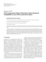
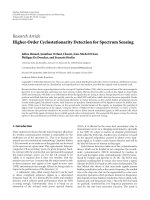
Figure 1: Block diagram of the proposed framework.
To implement this idea with the assumption of mel
frequency cepstral coefficients (MFCCs) feature extraction
and an HMM-based speech recognizer, we use an utterance
for which the transcription is given and formulate the
relation between SS filter parameters and the likelihood of
the correct model. The proposed method has two phases:
adaptation and decoding. In the adaptation phase, the spec-
tral oversubtraction factor is adjusted based on maximizing
the acoustic likelihood of the correct transcription. In the
decoding phase, in turn, the optimized filter is applied for
all incoming speech. Figure 1 shows the block diagram of the
proposed approach.
The remainder of this paper is organized as follows.
In Section 2, we review SS and multiband SS. Formulae
for maximum likelihood-based SS (MLBSS) are derived in
Section 3. Our proposed algorithm and its combination
with CMN technique are described in Sections 4 and 5,
respectively. Extensive experiments to verify the effectiveness
of our algorithm are presented in Section 6, and finally in
Section 7, we present the summary of our work.

2. Spectral Subtraction (SS)
SS is one of the most established and famous enhancement
methods in removing additive and uncorrelated noise from
noisy speech. SS divides the speech utterance into speech and
nonspeech regions. It first estimates the noise spectrum from
nonspeech regions and then subtracts the estimated noise
from the noisy speech and produces an improved speech
signal. Assume that clean speech s(t) is converted to noisy
speech y(t) by adding uncorrelated noise, n(t), where t is the
time index:
y(t)
= s(t)+n(t). (1)
Because the speech signal is nonstationary and time variant,
the speech signal is split into frames; then by applying
the Fourier transform and doing some approximations, we
obtain the below generalized formula
|Y
n
(k)|
T
∼
=
|
S
n
(k)|
T
+ |N
n
(k)|

T
,(2)
where n is the frame number and Y
n
(k), S
n
(k), and N
n
(k)are
the kth coefficient of the Fourier transform of the nth noisy
speech, clean speech, and noise frames, respectively, also T
is the power exponent. SS has two stages which we describe
briefly in the following subsections.
2.1. Noise Spectrum Update. Because estimating the noise
spectrum is an essential part of the SS algorithm, many
methods have been proposed [41, 42]. One of the most
common methods, which is the one used in this paper, is
given by [28]
|N
n
(k)|
T
=
⎧
⎪
⎪
⎨
⎪
⎪
⎩

(1 − λ)|N
n−1
(k)|
T
+ λ|Y
n
(k)|
T
if |Y
n
(k)|
T
<β|N
n
(k)|
T
,
|N
n−1
(k)|
T
otherwise,
(3)
where
|N
n
(k)| is the absolute value of the kth Fourier
transform coefficient of the nth noisy speech frame, and
0
≤ λ ≤ 1 is the updating noise factor. If a large λ is chosen,

the estimated noise spectrum changes rapidly and may result
in poor estimation. On the other hand, if a small λ is chosen,
despite the increased robustness in estimation when the noise
spectrum is stationary or changes slowly in time, it does not
permit the system to follow rapid noise changes. In turn, β
is the threshold parameter for distinguishing between noise
and speech signal frames.
2.2. Noise Spectrum Subtraction. After noise spectrum esti-
mation, we should estimate the clean speech spectrum, S
n
(k),
using
|S
n
(k)|
T
=
⎧
⎪
⎪
⎨
⎪
⎪
⎩
|
Y
n
(k)|
T
− α|N

n
(k)|
T
if |Y
n
(k)|
T
−α|N
n
(k)|
T
>γ|Y
n
(k)|
T
,
γ
|Y
n
(k)|
T
otherwise,
(4)
4 EURASIP Journal on Advances in Signal Processing
where α is the oversubtraction factor chosen to be between
0 and 3 and is used to compensate for mistakes in noise
spectrum estimation. Therefore, in order to obtain better
results, we should set this parameter accurately and adap-
tively. The parameter γ is the spectral floor factor which
is a small positive number assuring that the estimated

spectrum will not be negative. We estimate the initial
noise spectrum by averaging the first few frames of the
speech utterance (assuming the first few frames are pure
noise). Usually for the parameter T,avalueof1or2is
chosen. We have T
= 1 yielding the original magnitude
SS and T
= 2 yielding the power SS algorithm. Errors
in determining nonspeech regions cause incorrect noise
spectrum estimation and therefore may result in distortions
in the processed speech spectrum. Spectral noise estimation
is sensitive to the spectral noise variation even when the
noise is stationary. This is due to the fact that the absolute
value of the noise spectrum may differ from the noise mean
causing negative spectral estimation. Although the spectral
floor factor γ prevents this, it may cause distortions in the
processed signal and may generate musical noise artifacts.
Since Boll’s [3] research was introduced, several variations
of the method were proposed in literature to reduce the
musical noise. These methods were developed to perform
noise suppression in autocorrelation, cepstral, logarithmic
and, subspace domains. A variety of preprocessing and
postprocessing methods attempt to reduce the presence of
musical noise while minimizing speech distortion [43–46].
2.3. Multiband Spectral Subtraction (MBSS). Basic SS
assumes that noise affects the whole speech spectrum equally.
Consequently, it uses a single value of the oversubtraction
factor for the whole speech spectrum. Real world noise
is mostly colored and does not affect the speech signal
uniformly over the entire spectrum. Therefore, this suggests

the use of a frequency-dependent subtraction factor to
account for different types of noise. The idea of nonlin-
ear spectral subtraction (NSS), proposed in [7], basically
extends this capability by making the oversubtraction factor
frequency dependent and subtraction process nonlinear.
Larger values are subtracted at frequencies with low SNR
levels, and smaller values are subtracted at frequencies with
high SNR levels. Certainly, this gives higher flexibility in
compensating for errors in estimating the noise energy in
different frequency bins.
The motivation behind the MBSS approach is similar to
that of NSS. The main difference between MBSS and NSS
is that the MBSS approach estimates one oversubtraction
factor for each frequency band, whereas the NSS approach
estimates one oversubtraction factor for each individual Fast
Fourier Transform (FFT) bin. Different approaches based on
MBSS have been proposed. In [47], the speech spectrum
is divided into a considerably large number of bands, and
afixedvaluefortheoversubtractionfactorisusedforall
bands. In Kamath and Loiziou’s method [29], an optimum
oversubtraction factor is computed for each band based on
the SNR. Another method (similar to the work presented in
[29]) proposed in [48] uses the Berouti et al. SS method [28]
on each critical band over the speech spectrum.
We select the MBSS approach because it is computa-
tionally more efficient in our proposed framework. Also,
as reported in [49], the speech distortion is expected to be
markedly reduced with the MBSS approach. In this work,
we divide the speech spectrum using mel-scale frequency
bands (inspired by the structure of the human ear cochlea

[29]) and use a separate oversubtraction factor for each band.
Therefore, oversubtraction vector is defined as
α
= [α
1
, α
2
, , α
B
], (5)
where B is the number of the frequency bands. From
this section we conclude that the oversubtraction factor
is the most effective parameter in the SS algorithm. By
adjusting this parameter for each frequency band, we can
expect remarkable improvement in performance of speech
recognition systems. In the next section, we present a
novel framework for optimizing vector α based on feedback
information from the speech recognizer back end.
3. Maximum Likelihood-Based Spectral
Subtraction (MLBSS)
Conventional SS uses waveform-level criteria, such as maxi-
mizing signal to noise ratio or minimizing mean square error,
and tries to decrease the distance between noisy speech and
the desired speech. As mentioned in the introduction, using
these criteria should not necessarily decrease word error
rate. Therefore, in this paper, instead of a waveform-level
criterion, we use a word-error-rate criterion for adjusting the
spectral oversubtraction vector. One logical way to achieve
this goal is to select the oversubtraction vector in a way
that the acoustic likelihood of the correct hypothesis in

the recognition procedure is maximized. This will increase
the distance between the acoustic likelihood of the correct
hypothesis and other competing hypotheses, such that the
probability that the utterance be correctly recognized will
be increased. To implement this idea, the relation between
the oversubtraction factor in the preprocessing stage and the
acoustic likelihood of the correct hypothesis in the decoding
stage is formulated. The derived formulae depend on the
feature extraction algorithm and the acoustic unit model.
In this paper, MFCCs serve as the extracted features and
hidden Markov models with Gaussian mixtures in each state
as acoustic unit models. Speech recognition systems based
on statistical models find the word sequence most likely to
generate the observation feature vectors Z
={z
1
, z
2
, , z
t
}
extracted from the improved speech signal. These observa-
tion features are a function of both the incoming speech
signal and the oversubtraction vector. Statistical speech
recognizers obtain the most likely hypothesis based on Bayes’
classification rule:
w = arg max
w
P(Z(α) | w)P(w), (6)
where the observation feature vector is a function of

oversubtraction vector α.In(6), P(Z(α)
| w)andP(w)
are the acoustic and language scores, respectively. Our
goal is to find the oversubtraction vector α that achieves
EURASIP Journal on Advances in Signal Processing 5
the best recognition performance. Similar to both speaker
and environmental adaptation methods for the adjusting
oversubtraction vector α, we need access to adaptation data
with known phoneme transcriptions. We assume that the
correct transcription of the utterance w
C
is known. Hence,
the value of P(w
C
) can be ignored since it is constant
regardless of the value of α. We can then maximize (6)with
respect to α as
α = argmax
α
(P(Z(α) | w
C
)). (7)
In an HMM-based speech recognition system, the acoustic
likelihood P(Z(α)
| w
C
) is the sum of all possible
state sequences for a given transcription. Since most state
sequences are unlikely, we assume that the acoustic likelihood
of the given transcription is estimated by the single most

likely state sequence; such assumption also reduces compu-
tational complexity. If S
C
represents all state sequences in the
combinational HMM and s represents the most likely state
sequence, then the maximum likelihood estimation of α is
given by
α = argmax
α, s∈S
C


i
log

P(z
i
(α) | s
i
)

+

i
log

P(s
i
| s
i−1

, w
C
)


.
(8)
According to (8), in order to find
α, the acoustic likelihood of
the correct transcription should be jointly maximized with
respect to the state sequence and α parameters. This joint
optimization has to be performed iteratively.
In (8), the maximum likelihood estimation of
α may
become negative. This usually happens when test speech
data is cleaner than train speech data, for example, when
we train the acoustic model by noisy speech and use it
in clean environment. In such cases, the oversubtraction
factor is negative and adds noise to the speech spectrum,
but this is not an undesired effect; in fact, this is one of
the most important advantages of our algorithm because
adding noise PSD to the noisy speech spectrum decreases
the mismatch and consequently results in better recognition
performance.
3.1. State Sequence Optimization. Noisy speech is passed
through the SS filter, and feature vectors Z(α) are obtained
for a given value α. Then optimal state sequence s
=
{
s

1
, s
2
, , s
t
} is computed using (9) given the correct
phonetic transcription, w
C
:
s = arg max
s∈S
C


i
log

P(z
i
(α) | s
i
)

+

i
log

P(s
i

| s
i−1
, w
C
)


.
(9)
State sequence
s can be simply computed using the Viterbi
algorithm [50].
3.2. Spectral Oversub traction Vector Optimization. Given the
state sequence
s,wewanttofindα so that
α = argmax
α


i
log(P(z
i
(α) | s
i
))

. (10)
This acoustic likelihood can not be directly optimized with
respect to the SS parameters for two reasons. First, the
statistical distributions in each HMM state are complex

density functions such as mixture of Gaussians. Second,
some linear and nonlinear mathematical operations should
be performed on the speech signal for extracting feature
vectors, that is, the acoustic likelihood of the speech signal
is influenced by the α vector. Therefore, obtaining a closed-
form solution for computing the optimal α given a state
sequence is not possible; hence, nonlinear optimization is
used.
3.2.1. Computing Gradient Vector. We use gradient-based
approach to find the optimal value of the α vector. Given
an optimal state sequence in the combinational HMM, we
define L(α) to be the total log likelihood of the observation
vectors. Thus,
L(α)
=

i
log(P(z
i
(α) | s
i
)). (11)
The gradient vector
∇
α
L(α)iscomputedas
∇
α
L(α) =


∂L(α)
∂α
0
,
∂L(α)
∂α
1
, ,
∂L(α)
∂α
B−1

. (12)
Clearly, computing the gradient vector depends on both
the statistical distributions in each state and the feature
extraction algorithm. We derive
∇
α
L(α) assuming that
each state is modeled by K mixtures of multidimensional
Gaussians with diagonal covariance matrices. Let μ
ik
and

ik
be the mean vector and covariance matrix of the kth
Gaussian density function in state s
i
,respectively.Wecan
then write the sum of the acoustic likelihood given an

optimal state sequence s
={s
1
, s
2
, , s
t
} as
L(α)
=

i
log

K

k=1
exp(G
ik
(α))

, (13)
where G
ik
(α)isdefinedas
G
ik
(α)=exp

−

1
2
(z
i
(α)−μ
ik
)
T
−1

ik
((z
i
(α)−μ
ik
)+log(τ
ik
κ
ik
)

.
(14)
In (14), τ
ik
is the weight of the kth mixture in the ith state,
and κ
ik
is a normalizing constant. Using the chain rule, we
have

∇
α
L(α) =

i
K

k=1
γ
ik
(α)
∂G
ik
(α)
∂α
, (15)
where γ
ik
is defined as
γ
ik
=
exp(G
ik
(α))

K
j=1
exp(G
ij

(α))
. (16)
6 EURASIP Journal on Advances in Signal Processing
∂G
ik
(α)/∂α is derived as
∂G
ik
(α)
∂α
=
∂z
i
(α)
∂α
−1

ik
(z
i
(α) − μ
ik
). (17)
By substituting (17) into (15), we get
∇
α
L(α) =

i
K


k=1
γ
ik
(α)
∂z
i
(α)
∂α
−1

ik
(z
i
(α) − μ
ik
). (18)
In (18), ∂z
i
(α)/∂α is the Jacobian matrix, as in (19),
comprised of partial derivatives of each element of the ith
frame feature vector with respect to each component of the
oversubtraction vector α:
J
i
=
∂z
i
∂α
=

⎛
⎜
⎜
⎜
⎜
⎜
⎜
⎜
⎜
⎜
⎜
⎜
⎜
⎜
⎜
⎝
∂z
0
i
∂α
0
∂z
1
i
∂α
0
···
∂z
C−1
i

∂α
0
∂z
0
i
∂α
1
∂z
1
i
∂α
1
···
∂z
C−1
i
∂α
1
.
.
.
.
.
.
···
.
.
.
∂z
0

i
∂α
B−1
∂z
1
i
∂α
B−1
···
∂z
C−1
i
∂α
B−1
⎞
⎟
⎟
⎟
⎟
⎟
⎟
⎟
⎟
⎟
⎟
⎟
⎟
⎟
⎟
⎠

. (19)
The dimensionality of the Jacobian matrix is B
×C,whereB is
the number of elements in vector α and C is the dimension of
the feature vector. The full derivation of the Jacobian matrix
when the feature vectors are MFCC is given in the following
subsection.
3.2.2. Computing Jacobian Matrices. Every element of the
feature vector is a function of all elements of the α vector.
Therefore, to compute each element of the Jacobian matrix,
we should derive formulas for the derivation of the feature
vector from the SS output. Assume that x[n] is the input
signal and X[k] is its Fourier transform. We set the number
of frequency bands in multiband SS equal to the number
of mel filters, that is, for each mel filter we have one SS
filter coefficient. Since mel filters are a series of overlapping
triangular weighting functions, we define
α
j
[k]as
α
j
[k] =

α
j
ω
j
≤ k ≺ ω
j+1

,
0 otherwise,
(20)
where ω
j
and ω
j+1
are lower and upper bound of the jth mel
filter. The output of the SS filter, Y[k], is computed as
|Y(k)|
2
=

|X[k]|
2
−
B

j=1
α
j
[k]
β[k]
|N[k]|
2

×
U

|

X[k]|
2
−
B

j=1
α
j
[k]
β[k]
|N[k]|
2

+ |X[k]|
2
U

B

j=1
α
j
[k]
β[k]
|N[k]|
2
−|X[k]|
2

,

(21)
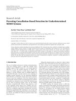
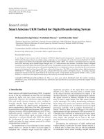
where U is the step function,
|N[k]|
2
is the average noise
spectrum of frames labeled as silence, and β[k] is the
1112222222222222222222222222222222222222221111111
β[k]
1
Figure 2: Schematic of β vector.
kth element of the β vector having the value of 2 in the
overlapping parts of the mel filter and value of 1 otherwise
(Figure 2).
The gradient of
|Y(k)|
2
with respect to elements of the α
vector is found as
∂Y
2
i
[k]
∂α
j
=
⎧
⎪
⎨
⎪
⎩

−|
N(k)|
2
β[k]
if ω
j
≤ k ≺ ω
j+1
,
0 otherwise.
(22)
In our experiments, ten frames from the beginning of the
speech signal are assumed to be silence. We update the
noise spectrum using (3), and the lth component of the mel
spectral vector is computed as
M
l
i
=
N/2

k=0

v
l
[k] ·|Y
i
[k]|
2


,0≤ l ≤ L − 1, (23)
where v
l
[k] is the coefficient of the lth triangular mel filter
bank and N is the number of Fourier transform coefficients.
We calculate the gradient of (23)withrespecttoα as
∂M
l
i
∂α
j
=
N/2

k=0
v

[k]
∂Y
2
i
[k]
∂α
j
=−
N/2

k=0
v


[k]|N[k]|
2
β[k]
. (24)
We can obtain the cepstral vector by first computing the
logarithm of each element of the mel spectral vector and then
performing a DCT operation as
∂z
c
i
∂α
j
=
L−1

=0
Φ
cl
M
l
i
∂M
l
i
∂α
j
=−
l−1

=0

Φ
cl
M
l
i
N/2

k=0
v

[k]|N[k]|
2
β[k]
, (25)
where Φ is a DCT matrix with dimension C
∗ L.
Using the gradient vector defined in (18), the α vector
can be optimized using the conventional gradient-based
approach. In this work, we perform optimization using the
method of conjugate gradients.
In this section, we introduced MLBSS—a new approach
to SS designed specifically for improved speech recognition
performance. This method differsfrompreviousSSalgo-
rithms in that waveform-level criteria are used to optimize
the SS parameters. Instead, the SS parameters are chosen
to maximize the likelihood of the correct transcription of
the utterance, as measured by the statistical models used by
the recognizer itself. We showed that finding a solution to
EURASIP Journal on Advances in Signal Processing 7
Spectral subtraction optimization block

Initial
parameters
False
True
Stop
Start
Estimate state sequence
Spectral subtraction
optimization
Desired
error rate?
spectral subtraction
Feature
extraction
Computing total
log likelihood
Total log
likelihood
converges?
Compute gradient of the
over - subtraction vector
Update over -
subt
raction vector
False
True
Details
Multiband
Multiband
spectral subtraction

User says an utterance with
a known transcription
Test on validation set
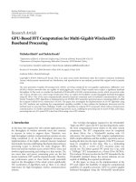
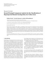
Figure 3: Flowchart of the proposed MLBSS algorithm.
this problem involves the joint optimization of the α vector,
as the SS parameters, and the most likely state sequence
for the given transcription. It was performed by iteratively
estimating the optimal state sequence for a given α vector
using the Viterbi algorithm and optimizing the likelihood
of the correct transcription with respect to the α vector for
that state sequence. For the reasons originally discussed in
Section 3.2, the likelihood of the correct transcription cannot
be directly maximized with respect to the α vector, and
therefore we do so using conjugate gradient descent as our
optimization method. Therefore, in Section 3.2,wederived
the gradient of the likelihood of the correct transcription
with respect to the α vector.
4. MLBSS Algorithm in Practice
In Section 3, a new approach to MBSS was presented in
which the SS parameters are optimized specifically for speech
recognition performance using feedback information from
the speech recognition system. Specifically, we showed how
the SS parameters (vector α) can be optimized to maximize
the likelihood of an utterance with known transcription.
Obviously, here we should answer the following question: if
the correct transcription is known a priori, why should there
be any need for recognition? The answer is that the correct
transcription is only needed in the adaptation phase. In
the decoding phase, the filter parameters are fixed. Figure 3
shows the flowchart of our proposed algorithm.

First, the user is asked to speak an utterance with a
known transcription. The utterance is then passed through
the SS filter with fixed initial parameters. After that, the
most likely state sequence is generated using the Viterbi [50]
algorithm. The optimal SS filter is then produced given the
state sequence. Recognition is performed on a validation set
using the obtained optimized filter. If the desired word error
rate is reached the algorithm is finished, otherwise the new
state sequence is estimated.
Figure 3 also shows the details of the SS optimization
block. This block iteratively finds the oversubtraction vector
which maximizes the total log likelihood of the utterance
with a given transcription. First, the feature vector is
extracted from the improved speech signal, and then the
log likelihood is computed given the state sequence. If the
likelihood does not converge, the gradient of the oversub-
traction vector is computed, and the oversubtraction vector
is updated. SS is performed with the updated parameters,
and new feature vectors are extracted. This process is
repeated until the convergence criterion is satisfied.
In the proposed algorithm, similar to speaker and envi-
ronment adaptation techniques, the oversubtraction vector
adaptation can be implemented either in a separate off-
line session or by embedding an incremental on-line step to
the normal system recognition mode. In off-line adaptation,
as explained above, the user is aware of the adaptation
process typically by performing a special adaptation session,
while in on-line adaptation the user may not even know
that adaptation is carried out. On-line adaptation is usually
embedded in the normal functioning of a speech recognition

system. From a usability point of view, incremental on-
line adaptation provides several advantages over the off-line
approach making it very attractive for practical applications.
Firstly, by means of on-line adaptation, the adaptation
process is hidden from the user. Secondly, the use of on-line
adaptation allows us to improve robustness against chang-
ing noise conditions, channels, and microphones. Off-line
8 EURASIP Journal on Advances in Signal Processing
adaptation is usually done as an additional training session
in a specific environment, and thus it is not possible to
incorporate new environment characteristics for parameter
adaptation.
The adaptation data can be aligned with HMMs in
two different ways. In supervised adaptation, the identity
of the adaptation data is always known, whereas in the
unsupervised case it is not; hence, adaptation utterances
are not necessarily correctly aligned. Supervised adaptation
is usually slow particularly with speakers whose utterances
result in poor recognition performance because only the
correctly classified utterances are utilized in adaptation.
5. Combination of MLBSS and CMN
In the MLBSS algorithm described in Sections 3 and 4,
relations were derived under the assumption of additive
noise. However, in some application such as distant-talking
speech recognition, it is necessary to cope not only with
additive noise but also with the acoustic transfer function
(channel noise). CMN [18] is a simple (low computational
cost and easy to implement) yet very effective method for
removing convolutional noise, such as distortions caused
by different recording devices and communication channels.

Due to the presence of the natural logarithm in the
feature extraction process, linear filtering usually results in
a constant offset in the filter bank or cepstral domains and
hence can be subtracted from the signal. The basic CMN
estimates the sample mean vector of the cepstral vectors of
an utterance and then subtracts this mean vector from every
cepstral vector of the utterance. We can combine CMN with
the proposed MLBSS method by mean normalization of the
Jacobian matrix. Let
z
i
(α) be the mean normalized feature
vector:
z
i
(α) = z
i
(α) −
1
T
T

i=1
z
i
(α). (26)
The partial derivative of
z
i
(α) with respect to α can be

computed as
∂
z
i
(α)
∂α
=
∂z
i
(α)
∂α
−
1
T
T

i=1
∂z
i
(α)
∂α
, (27)
where this equation is equal to mean normalization of the
Jacobian matrix.
Hence, features mean normalization can easily be incor-
porated into the MLBSS algorithm presented in Section 4.To
do so, the feature vector z
i
(α)in(11)isreplacedby(z
i

(α) −
μ
z
(α)) where μ
z
(α) is the mean feature vector, computed over
all frames in the utterance. Because μ
z
(α) is a function of α as
well, the gradient expressions also have to be modified. Our
experimental results have shown that in real environments
better results are obtained when MLBSS and CMN are used
together properly.
6. Experimental Results
In this section, the proposed MLBSS algorithm is evaluated
and is also compared with traditional SS methods for speech
recognition using a variety of experiments. In order to
assess the effectiveness of the proposed algorithm, speech
recognition experiments were conducted on three speech
databases: FARSDAT [51], TIMIT [52], and a recorded
database in a real office environment. The first and second
test sets are obtained by artificially adding seven types of
noises (alarm, brown, multitalker, pink, restaurant, volvo,
and white noise) from the NOISEX-92 database [53]to
the FARSDAT and TIMIT speech databases, respectively.
The SNR was determined by the energy ratio of the clean
speech signal including silence periods and the added noise
within each sentence. Practically, it is desirable to measure
the SNR by comparing energies during speech periods only.
However, on our datasets, the duration of silence periods

in each sentence was less than 10% of the whole sentence
length; hence, the inclusion of silence periods is considered
acceptable for relative performance measurement. Sentences
were corrupted by adding noise scaled on a sentence-by-
sentence basis to an average power value computed to
produce the required SNR.
Speech recognition experiments were conducted on
Nevisa [54], a large-vocabulary, speaker-independent, con-
tinuous HMM-based speech recognition system developed
in the speech processing lab of the Computer Engineering
Department of Sharif University of Technology. Also, it was
the first system to demonstrate the feasibility of accurate,
speaker-independent, large-vocabulary continuous speech
recognition in Persian language. Experiments have been
done in two different operational modes of the Nevisa
system: phoneme recognition on FARSDAT and TIMIT
databases and isolated command recognition on a distant
talking database recorded in a real noisy environment.
The reason for reporting phoneme recognition accuracy
results instead of word recognition accuracy is that in the
former case the recognition performance lies primarily on
the acoustic model. For word recognition, the performance
becomes sensitive to various factors such as the language
model type. The phoneme recognition accuracy is calculated
as follows:
Accuracy (%)
=
N − S − D − I
N
∗ 100%, (28)

with S, D,andI being the number of substitution, deletion,
and insertion errors, and N the number of test phonemes.
6.1. Evaluation on Added-Noise Conditions. In this section,
we describe several experiments designed to evaluate the
performance of the MLBSS algorithm. We explore sev-
eral dimensions of the algorithm including the impact of
SNR and type of added noises on recognition accuracy,
performance of the single-band version of the algorithm,
recognition accuracy of the algorithm on a clean test set, and
test sets with various SNR levels when models are trained in
noisy conditions.
The experiments described herein were performed using
the hand-segmented FARSDAT database. This database
consists of 6080 Persian utterances, uttered by 304 speakers.
Speakers are chosen from 10 different geographical regions
in Iran; hence, the database incorporates the 10 most
EURASIP Journal on Advances in Signal Processing 9
common dialects of the Persian language. The male-to-
female population ratio is two to one. There are a total of
405 sentences in the database and 20 utterances per speaker.
Each speaker has uttered 18 randomly chosen sentences
plus two sentences which are common for all speakers.
Sentences are formed by using over 1000 Persian words. The
database is recorded in a low-noise environment with an
average SNR of 31 dB. One can consider FARSDAT as the
counterpart of TIMIT in Persian language. Our clean test
set is selected from this database and is comprised of 140
sentences from 7 speakers. All of the other sentences are used
as a training set. To simulate a noisy environment, testing
data was contaminated by seven types of additive noises at

several SNRs ranging from 0 dB to 20 dB with 5 dB steps to
produce various noisy test sets. Therefore, the test set does
not consider the effect of stress or the Lombard effect on the
production of speech in noisy environments.
The Nevisa speech recognition engine was used for our
experiments. The feature set used in all the experiments
was generated as follows. The speech signal, sampled at
22050 Hz, is applied to a pre-emphasis filter and blocked
into frames of 20 milliseconds with 12 ms of overlap. A
Hamming window is also applied to the signal to reduce the
effect of frame edge discontinuities, and a 1024-point FFT
is calculated. The magnitude spectrum is warped according
to the mel scale. The obtained spectral magnitude spectrum
is integrated within 25 triangular filters arranged on the mel
frequency scale. The filter output is the logarithm of the sum
of the weighted spectral magnitudes. A decorrelation step is
performed by applying a discrete cosine transform. Twelve
MFCCs are computed from the 25 filter outputs [53]. First-
and second-order derivatives of the cepstral coefficients are
calculated over a window covering five neighbouring cepstral
vectors to make up vectors of 36 coefficients per speech
frame.
Nevisa uses continuous density hidden Markov modeling
with each HMM representing a phoneme. Persian language
consists of 29 phonemes. Also, one model was used to
represent silence. All HMMs are left to right and they are
composed of 5 states and 8 Gaussian mixtures in each state.
Forward and skip transitions between the states and self-
loop transitions are allowed. Covariance of each Gaussian
is modeled by a single diagonal matrix. The initialization of

parameters is done using linear segmentation, and the seg-
mental k-means algorithm is used to estimate the expected
parameters after 10 iterations. The Nevisa decoding process
consists of a time-synchronous Viterbi beam search.
One of the 140 sentences of the test set is used in the
optimization phase of the MLBSS algorithm. After filter
parameters are extracted, speech recognition is performed
on the remaining test set files using the obtained optimized
filter. Tab le 1 shows phoneme recognition accuracy for the
test speech files. To evaluate our algorithm, our results are
compared with the Kamath and Loizou’s [29]multiband
spectral subtraction (KLMBSS) method which uses an
SNR-based optimization criterion. In the KLMBSS method
implementation, the speech signal is first Hamming win-
dowed using a 20-millisecond window and a 10-millisecond
overlap between frames. The windowed speech frame is
0
10
20
30
40
50
60
70
80
90
100
Phoneme recognition rate (%)
0 5 10 15 20
SNR (dB)

Berouti’s SS
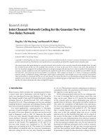
MLBSS
Figure 4: Phoneme recognition accuracy rate (%) as function of
SNR with Berouti et al.’s speech enhancement approach and single-
band MLBSS scheme.
then analyzed using the FFT. The resulting spectrum and
the estimated noise spectrum are divided into 25 frequency
bands using the same mel spacing as the MLBSS method.
The estimate of the clean speech spectrum in the ith band
is obtained by
|S
i
(k)|
2
=
⎧
⎪
⎪
⎨
⎪
⎪
⎩
|
Y
i
(k)|
2
− α
i
δ

i
|N
i
(k)|
2
if |Y
i
(k)|
2
− α
i
δ
i
|N
i
(k)|
2
> 0,
β
|Y
i
(k)|
2
otherwise,
(29)
where α
i
is the oversubtraction factor of the ith band, δ
i
is

a bandsubtraction factor, and β is a spectral floor parameter
that is set to 0.002.
From the experimental results, as shown in Ta bl e 1 ,we
observe the following facts. With regards to various noise
types and various SNRs, results show that the proposed
method was capable of improving recognition performance
relative to a classical method. In some cases, Kamath
and Loizou’s method achieves lower performance than the
baseline. This is due to spectral distortions caused by not
adjusting the oversubtraction factors thus destroying the
discriminability used in pattern recognition. This mismatch
reduces the effectiveness of the clean trained acoustical
models and causes recognition accuracy to decline. Higher
SNR differences between training and testing speech cause
a higher degree of mismatch and greater degradation in the
recognition performance.
6.2. Evaluation on Single Band Conditions. In order to show
the efficiency of the MLBSS algorithm for optimizing single
band SS, we compare the results of the proposed method
operating in single-band mode with Berouti et al.’s SS
[28] which is a single-band SNR-based method. Results
are shown in Figure 4. An inspection of this figure reveals
that single-band MLBSS scheme consistently performs better
than the SNR-based Berouti et al.’s approach in noisy speech
environments across a wide range of SNR values.
10 EURASIP Journal on Advances in Signal Processing
Table 1: Phoneme recognition accuracy (%) on FARSDAT database.
Noisetype Method 0dB 5dB 10dB 15dB 20dB
Alarm
No enhance 34.49 43.89 52.94 59.40 66.09

KLMBSS 34.56 45.19 53.64 59.73 66.17
MLBSS 35.01 46.64 55.06 61.80 68.32
Brown
No enhance 64.99 72.61 76.07 77.16 77.34
KLMBSS 66.66 73.19 75.84 77.56 77.16
MLBSS 67.30 75.76 78.76 79.34 79.68
Multitalker
No enhance 32.41 42.62 52.71 61.01 67.47
KLMBSS 33.56 44.62 52.51 62.90 68.65
MLBSS 33.79 46.23 56.56 64.69 70.45
Pink
No enhance 21.34 31.37 44.35 55.59 69.84
KLMBSS 22.78 35.33 47.27 60.09 69.07
MLBSS 23.24 37.06 49.98 62.92 74.20
Restaurant
No enhance 32.24 41.70 52.48 61.94 70.24
KLMBSS 33.58 45.59 55.88 63.85 70.20
MLBSS 34.14 46.12 56.21 66.59 73.45
Vo lv o
No enhance 62.17 65.34 68.86 75.20 76.36
KLMBSS 63.09 68.03 71.17 74.88 76.78
MLBSS 63.61 68.78 72.01 76.39 78.82
White
No enhance 19.43 31.37 43.25 54.61 66.32
KLMBSS 19.57 30.83 42.28 53.66 63.55
MLBSS 22.84 36.78 48.02 59.50 70.86
Table 2: Phoneme recognition accuracy rate (%) in clean environ-
ment.
Dataset No enhance KLMBSS MLBSS
TIMIT 66.43 53.75 66.79

FARSDAT 77.28 76.24 77.36
6.3. Experimental Results in Clean Environment. Front-end
processing to increase noise robustness can sometimes
degrade recognition performance under clean test condi-
tions. This may occur as speech enhancement methods
such that SS can generate unexpected distortions for clean
speech. As a consequence, Even though the performance
of an MLBSS algorithm is considerably good under noisy
environments, it is not desirable if the recognition rate
decreases for clean speech. For this reason, we evaluate
the performance of the MLBSS algorithm not only in
noisy conditions but also on the clean original TIMIT and
FARSDAT databases. Recognition results obtained from the
clean conditions are shown in Ta bl e 2 where we can find
that the recognition accuracy of the MLBSS approach is even
a bit higher than that of the baseline while the KLMBSS
method shows noticeable decline. This phenomenon can
be interpreted that the MLBSS approach has the ability to
compensate for the effects of noise, so only the mismatch is
reduced.
6.4. Experimental Results in Noisy Training Conditions. In
this section, we evaluate the performance of the MLBSS
algorithm in noisy training conditions by using noisy speech
data in the training phase. Recognition results obtained
from the noisy training conditions are shown in Figure 5,
where the following deductions can be made: (i) higher SNR
difference between the training and testing speech causes
higher degree of mismatch, and therefore results in greater
degradation in recognition performance; (ii) in matched
conditions, where the recognition system is trained with

speech having the same level of noise as the test speech,
best recognition accuracies are obtained; (iii) the MLBSS
is more effective than the KLMBSS method in overcoming
environmental mismatch where models are trained with
noisy speech but the noise type and the SNR level of noisy
speech are not known a priori; (iv) in the KLMBSS method,
lower SNR of the training data results in greater degradation
in recognition performance.
6.5. On-Line MLBSS Framework Evaluation. In this exper-
iment, the performance of incremental on-line adaptation
under added noise conditions is compared to that of off-
line adaptation. In the case of supervised off-line adapta-
tion, the parameter update was based on one adaptation
utterance spoken in a noisy environment. As mentioned
in Section 5, after adaptation, an updated oversubtraction
EURASIP Journal on Advances in Signal Processing 11
0
10
20
30
40
50
60
70
80
90
100
Phoneme recognition rate (%)
0510
15 20 25

SNR (dB)
No enhance
KLMBSS
MLBSS
(a)
0
10
20
30
40
50
60
70
80
90
100
Phoneme recognition rate (%)
0510
15 20 25
SNR (dB)
No enhance
KLMBSS
MLBSS
(b)
Figure 5: Phoneme recognition accuracy rate (%) as a function of the signal-to-noise ratio of the speech being recognized, where the
recognition system has been trained on noisy speech. In (a) and (b), system has been trained with additive white noise at SNR 10 dB and
20 dB noisy speech, respectively.
Table 3: Phoneme recognition accuracy (%) in changing SNR conditions.
Noise type SNR
Approach

No enhance KLMBSS Off-line MLBSS On-line MLBSS
White 10 → 20 55.03 54.92 58.76 61.02
White 20
→ 10 57.36 57.68 60.71 62.24
Alarm 10
→ 20 58.42 59.15 61.09 63.83
Alarm 20
→ 10 60.22 61.21 63.11 65.16
vector is computed from the processed utterance, and this
new vector is subsequently used to recognize the remainder
of the test data. In the case of incremental on-line adaptation,
only correctly recognized test utterances are utilized for
adaptation (supervised approach). A new oversubtraction
vector is always computed after one correctly recognized
utterance has been processed.
In order to further evaluate the performance of the on-
line version of the proposed algorithm in noise varying
conditions, we carry out a number of experiments where
the SNR of the added noise was made artificially time
varying. For this, we varied the SNR linearly from an
initial value to final within each utterance. Recognition
results are shown in Tab le 3 where 10
→ 20 indicates
that the SNR was changed linearly within a sentence such
that it was 10 dB at the beginning and 20 dB at the end.
For this time-varying SNR condition, the on-line MLBSS
algorithm yielded the best recognition performance among
the evaluated approaches when white noise was used. What
should be noted here is that the KLMBSS algorithm resulted
in only a modest improvement over the baseline for time-

varying SNR conditions; in fact, in the 10
→ 20 case, it even
decreased recognition performance.
6.6. Evaluation on TIMIT Database. All the above experi-
ments were done on the FARSDAT database which is the
counterpart of TIMIT for Persian language. In order to
verify the performance of the MLBSS algorithm, the same
experiments as those described in Section 6.1 were devised
on the TIMIT database and were conducted using the
Nevisa system. The results are reported in Ta bl e 4 .Ascanbe
seen, the obtained results are in agreement with the results
obtained with the FARSDAT database.
It can be concluded from the aforementioned experi-
ments that the MLBSS algorithm has the capability to signif-
icantly increase the robustness of the recognition system on
artificially noise-added data. However, a direct comparison
is still missing as the desired performance is needed for
real environments. Therefore, a third set of experiments was
performed and will be described below.
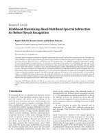
6.7. Evaluation on Data Recorded in Real Environment. To
formally quantify the performance of the proposed algo-
rithm in comparison with commonly used SS techniques,
speech recognition experiments were carried out on speech
data recorded in a real noisy office environment. The
experiments were specifically set up to generate a worst-
case scenario of combined interfering point source and
background noise to illustrate the potential of the robustness
scheme in a complex, real-life situation.
In this experiment, we used an isolated command
recognition task trained with clean isolated commands and

12 EURASIP Journal on Advances in Signal Processing
Table 4: Phoneme recognition accuracy (%) on TIMIT database.
Noise type Method 0 dB 5dB 10 dB 15 dB 20 dB
Alarm
No enhance 19.46 28.95 37.06 46.07 52.91
KLMBSS 20.16 27.47 38.21 45.06 49.33
MLBSS 21.42 31.97 40.38 48.25 54.97
Brown
No enhance 40.60 48.53 56.46 61.92 63.96
KLMBSS 40.72 49.09 53.29 54.67 54.97
MLBSS 43.12 54.31 60.56 64.58 65.05
Multitalker
No Enhance 13.99 23.60 34.35 43.78 51.89
KLMBSS 14.04 25.80 35.15 42.96 49.45
MLBSS 15.98 26.17 37.44 47.17 54.49
Pink
No enhance 8.85 13.29 20.68 28.49 37.86
KLMBSS 10.63 15.89 22.62 33.43 41.90
MLBSS 11.17 17.21 24.84 33.77 43.14
Restaurant
No enhance 13.33 20.78 30.15 40.00 48.89
KLMBSS 16.34 25.47 33.81 40.30 46.07
MLBSS 16.71 25.76 34.43 42.22 50.09
Vo lv o
No enhance 44.44 48.59 53.39 57.36 61.02
KLMBSS 43.00 48.25 51.13 52.93 54.19
MLBSS 46.25 51.51 55.53 59.38 63.04
White
No Enhance 3.72 8.47 15.68 23.96 31.77
KLMBSS 5.11 9.61 20.90 25.72 35.98

MLBSS 5.86 11.91 22.38 28.31 36.29
tested with noisy data captured from a microphone placed
2 m away from the speaker. We collected the training dataset
using a close-talking microphone in a quiet office using
16 female and 32 male talkers; each uttered 30 commands
such as turn on/off or open/close different devices in an
office. We gathered the test data in the office environment
depicted in Figure 6. For the test set, 22 male and 11 female
talkers, different from those used to produce the training
dataset, uttered commands at a 2m distance from the
microphone. Room dimensions were 4.5 m
× 3.5 m × 3.5 m
which resulted in a reverberation time of approximately 300
milliseconds (T
60
∼
=
0.3 s). There were some sources of noise
such as 3 computers and a loudspeaker propagating office
noise from the NOISEX database at a 40-degree angle with
the wall. The average SNR of the test set was 15 dB. We
partitioned this test set into two sets, and MFCCs were cal-
culated. Speech recognition was performed using the Nevisa
system in isolated command recognition mode. Isolated
commands are modeled by fifteen states left-to-right HMMs
with no skip (2 Gaussians/state). CMN was performed on the
training utterances. The results of our different experiments
are shown in Figure 7. In all experiments, KLMBSS, MLBSS,
CMN, SS + CMN, and MLBSS + CMN are compared. Results
show that adding CMN to the enhancement techniques

compensates for the channel effect. This figure also shows
that combining CMN with MLBSS is more effective than all
other combinations and reduces the error rate by up to 35
percent relative to MLBSS alone and up to 44 percent relative
to the no-enhance baseline.
From these experiments, the following deductions can be
made: (i) each approach is able to improve the robustness of
the system; (ii) MLBSS combined with CMS yields the high-
est robustness to noise among the approaches investigated;
(iii) while the robustness of the MLBSS approach is slightly
inferior to that of the KMBSS, it yields better performance
when combined by CMS.
7. Summary
In this paper, we have proposed a likelihood-maximizing-
multiband spectral subtraction algorithm—a new approach
for noise robust speech recognition which integrates MBSS
and likelihood maximizing schemes. In this algorithm,
SS parameters are jointly optimized based on feedback
information from a speech recognizer. Therefore, speech
signals processed using the proposed algorithm are more
accurately recognized than those processed with conven-
tional SS methods. In all, the main advantage of the proposed
algorithm is that the SS parameters are adapted based on a
criterion much more correlated with the speech recognition
objective than the SNR criterion which is commonly used in
practice.
EURASIP Journal on Advances in Signal Processing 13
40
2 m
2 m

Noise
speaker
Speaker
4.5 m
3.5 m
Height of the room 3.5 m
Figure 6: Map of experimental room, showing the position of the
talker, noise source, and computers.
0
10
20
30
40
50
60
70
80
90
100
Error rate (%)
No
enhance
KLMBSS MLBSS
CMN
KLMBSS
+CMN
MLBSS
+CMN
Figure 7: Error rate (%) of the Nevisa system in isolated command
recognition operational mode on data recorded in real environment

versus different combinations of the proposed MLBSS algorithm,
KLMBSS, and CMN.
The proposed algorithm has been tested and compared
to classical SS algorithms using various noise types and SNR
levels. Experimental results show that the proposed algo-
rithm leads to considerable recognition rate improvements.
Hence, we can conclude that using feedback information
from a speech recognizer in the front-end enhancement pro-
cess can result in significant improvements when compared
to classical enhancement methods.
In future works, we are planning to evaluate discrimi-
native methods instead of likelihood maximizing schemes.
Another possible future extension of this work includes the
utilization of the uncertainty associated with the enhanced
features using an uncertainty decoding approach.
Acknowledgments
This research was in part supported by a grant from
Iran Telecommunication Research Center (ITRC). The first
author would also like to thank Tiago Falk and Ebrahim
Kazemzadeh for their valuable comments and careful proof-
reading of this paper.
References
[1] P. J. Moreno, Speech recognition in noisy environments,Ph.D.
dissertation, ECE Department, Carnegie Mellon University,
Pittsburgh, Pa, USA, 1996.
[2] B. Raj and R. M. Stern, “Missing-feature approaches in speech
recognition,” IEEE Signal Processing Magazine, vol. 22, no. 5,
pp. 101–116, 2005.
[3] S. Boll, “Suppression of acoustic noise in speech using spectral
subtraction,” IEEE Transactions on Acoustics, Speech, and

Signal Processing, vol. 27, no. 2, pp. 113–120, 1979.
[4] A. Fischer and V. Stahl, “On improvement measures for
spectral subtraction applied to robust automatic speech recog-
nition in car environments,” in Proceedings of the Workshop on
Robust Methods for Speech Recognition in Adverse Conditions,
pp. 75–78, Tampere, Finland, May 1999.
[5] J. Huang and Y. Zhao, “An energy-constrained signal subspace
method for speech enhancement and recognition in white and
colored noises,” Speech Communication, vol. 26, no. 3, pp. 165–
181, 1998.
[6] W. M. Kushner, V. Goncharoff,C.Wu,V.Nguyen,andJ.N.
Damoulakis, “The effects of subtractive-type speech enhance-
ment/noise reduction algorithms on parameter estimation
for improved recognition and coding in high noise environ-
ments,” in Proceedings of the IEEE International Conference on
Acoustics, Speech, and Signal Processing (ICASSP ’89), vol. 1,
pp. 211–214, Glasgow, Scotland, May 1989.
[7] P. Lockwood and J. Boudy, “Experiments with a nonlinear
spectral subtractor (NSS), hidden Markov models and the
projection, for robust speech recognition in cars,” Speech
Communication, vol. 11, no. 2-3, pp. 215–228, 1992.
[8] C. Ris and S. Dupont, “Assessing local noise level estimation
methods: application to noise robust ASR,” Speech Communi-
cation, vol. 34, no. 1-2, pp. 141–158, 2001.
[9] E. Visser, M. Otsuka, and T W. Lee, “A spatio-temporal speech
enhancement scheme for robust speech recognition in noisy
environments,” Speech Communication,vol.41,no.2-3,pp.
393–407, 2003.
[10] J. Porter and S. Boll, “Optimal estimators for spectral restora-
tion of noisy speech,” in Proceedings of the IEEE Interna-

tional Conference on Acoustics, Speech, and Signal Processing
(ICASSP ’84) , vol. 9, pp. 53–56, San Diego, Calif, USA, March
1984.
[11] V. Stahl, A. Fischer, and R. Bippus, “Quantile based noise
estimation for spectral subtraction and Wiener filtering,” in
Proceedings of the IEEE International Conference on Acoustics,
Speech, and Signal Processing (ICASSP ’00), vol. 3, pp. 1875–
1878, Istanbul, Turkey, June 2000.
[12] Y. Ephraim, D. Malah, and B H. Juang, “On the application
of hidden Markov models for enhancing noisy speech,” IEEE
Transactions on Acoustics, Speech, and Signal Processing, vol. 37,
no. 12, pp. 1846–1856, 1989.
[13] H. Sameti, H. Sheikhzadeh, L. Deng, and R. L. Brennan,
“HMM-based strategies for enhancement of speech signals
embedded in nonstationary noise,” IEEE Transactions on
Speech and Audio Processing, vol. 6, no. 5, pp. 445–455, 1998.
[14] V. Stouten, H. Van hamme, and P. Wambacq, “Model-based
feature enhancement with uncertainty decoding for noise
robust ASR,” Speech Communication, vol. 48, no. 11, pp. 1502–
1514, 2006.
[15] A. Acero, Acoustical and Environmental Robustness in Auto-
matic Speech Recognition, Kluwer Academic Publishers, Nor-
well, Mass, USA, 1993.
14 EURASIP Journal on Advances in Signal Processing
[16] P. J. Moreno, B. Raj, and R. M. Stern, “Data-driven envi-
ronmental compensation for speech recognition: a unified
approach,” Speech Communication, vol. 24, no. 4, pp. 267–285,
1998.
[17] P.J.Moreno,B.Raj,E.Gouvea,andR.M.Stern,“Multivariate-
Gaussian-based cepstral normalization for robustspeech

recognition,” in Proceedings of the International Conference on
Acoustics, Speech, and Signal Processing (ICASSP ’95) , vol. 1,
pp. 137–140, Detroit, Mich, USA, May 1995.
[18] S. Furui, “Cepstral analysis technique for automatic speaker
verification,” IEEE Transactions on Acoustics, Speech, and
Signal Processing, vol. 29, no. 2, pp. 254–272, 1981.
[19] H. Hermansky, “Perceptual linear predictive (PLP) analysis of
speech,” Journal of the Acoustical Society of America, vol. 87, no.
4, pp. 1738–1752, 1990.
[20] H. Hermansky and N. Morgan, “RASTA processing of speech,”
IEEE Transactions on Speech and Audio Processing,vol.2,no.4,
pp. 578–589, 1994.
[21] M. J. F. Gales and S. J. Young, “Robust continuous speech
recognition using parallel model combination,” IEEE Transac-
tions on Speech and Audio Processing, vol. 4, no. 5, pp. 352–359,
1996.
[22] A. P. Varga and R. K. Moore, “Hidden Markov model
decomposition of speech and noise,” in Proceedings of the
IEEE International Conference on Acoustics, Speech, and Signal
Processing (ICASSP ’90), vol. 2, pp. 845–848, Albuquerque,
NM, USA, April 1990.
[23] C. J. Leggetter and P. C. Woodland, “Speaker adaptation of
continuous density HMMs using multivariate linear regres-
sion,” in Proceedings of the 3rd International Conference
on Spoken Language Processing (ICSLP ’94), pp. 451–454,
Yokohama, Japan, September 1994.
[24] H. Misra, Multi-stream processing for noise robust speech
recognition, Ph.D. thesis, Swiss Federal Institute of Technology,
Zurich, Switzerland, 2006.
[25] M. Cooke, P. Green, L. Josifovski, and A. Vizinho, “Robust

automatic speech recognition with missing and unreliable
acoustic data,” Speech Communication, vol. 34, no. 3, pp. 267–
285, 2001.
[26] B. Raj, M. L. Seltzer, and R. M. Stern, “Reconstruction
of missing features for robust speech recognition,” Speech
Communication, vol. 43, no. 4, pp. 275–296, 2004.
[27] M. L. Seltzer, B. Raj, and R. M. Stern, “Likelihood-maximizing
beamforming for robust hands-free speech recognition,” IEEE
Transactions on Speech and Audio Processing,vol.12,no.5,pp.
489–498, 2004.
[28] M. Berouti, R. Schwartz, and J. Makhoul, “Enhancement of
speech corrupted by acoustic noise,” in Proceedings of the
IEEE International Conference on Acoustics, Speech, and Signal
Processing (ICASSP ’79), vol. 4, pp. 208–211, Washington, DC,
USA, April 1979.
[29] S. Kamath and P. Loizou, “A multi-band spectral subtraction
method for enhancing speech corrupted by colored noise,” in
Proceedings of the IEEE International Conference on Acoustics,
Speech, and Signal Processing (ICASSP ’02), pp. 4160–4164,
Orlando, Fla, USA, May 2002.
[30] B. L. Sim, Y. C. Tong, J. S. Chang, and C. T. Tan, “A parametric
formulation of the generalized spectral subtraction method,”
IEEE Transactions on Speech and Audio Processing,vol.6,no.4,
pp. 328–337, 1998.
[31] P. Sovka, P. Pollak, and J. Kybic, “Extended spectral subtrac-
tion,” in Proceedings of European Signal Processing Conference
(EUSIPCO ’96), pp. 963–966, Trieste, Italy, September 1996.
[32] Y. M. Cheng and D. O’Shaughnessy, “Speech enhancement
based conceptually on auditory evidence,” in Proceedings of the
IEEE International Conference on Acoustics, Speech, and Signal

Processing (ICASSP ’91), pp. 961–964, Toronto, Canada, April
1991.
[33] N. Virag, “Single channel speech enhancement based on
masking properties of the human auditory system,” IEEE
Transactions on Speech and Audio Processing,vol.7,no.2,pp.
126–137, 1999.
[34] J. Lim, “Evaluation of a correlation subtraction method for
enhancing speech degraded by additive white noise,” IEEE
Transactions on Acoustics, Speech, and Signal Processing, vol. 26,
no. 5, pp. 471–472, 1978.
[35] J. Chen, K. K. Paliwal, and S. Nakamura, “Sub-band based
additive noise removal for robust speech recognition,” in
Proceedings of the 7th European Conference on Speech Com-
munication and Technology (EUROSPEECH ’01), pp. 571–574,
Aalborg, Denmark, September 2001.
[36] M. Fujimoto, J. Ogata, and Y. Ariki, “Large vocabulary
continuous speech recognition under real environments using
adaptive sub-band spectral subtraction,” in Proceedings of the
6th International Conference on Spoken Language Processing
(ICSLP ’00), vol. 1, pp. 305–308, Beijing, China, October 2000.
[37] M. Kleinschmidt, J. Tchorz, and B. Kollmeier, “Combining
speech enhancement and auditory feature extraction for
robust speech recognition,” Speech Communication, vol. 34,
no. 1-2, pp. 75–91, 2001.
[38] S. V. Vaseghi and B. P. Milner, “Noise compensation methods
for hidden Markov model speech recognition in adverse envi-
ronments,” IEEE Transactions on Speech and Audio Processing,
vol. 5, no. 1, pp. 11–21, 1997.
[39] H. Yamamoto, M. Yamada, Y. Komiri, and Y. Ohora, “Esti-
mated segmental SNR base adaptive spectral subtraction

approach for speech recognition,” Tech. Rep. SP94-50, IEICE,
Tokyo, Japan, 1994.
[40] J. C. Junqua and J. P. Haton, Robustness in Automatic Speech
Recognition: Fundamentals and Applications,KluwerAcademic
Publishers, Norwell, Mass, USA, 1995.
[41] H. G. Hirsch and C. Ehrlicher, “Noise estimation techniques
for robust speech recognition,” in Proceedings of the IEEE
International Conference on Acoustics, Speech, and Signal
Processing (ICASSP ’95), vol. 1, pp. 153–156, Detroit, Mich,
USA, May 1995.
[42] S. Rangachari and P. C. Loizou, “A noise-estimation algorithm
for highly non-stationary environments,” Speech Communica-
tion, vol. 48, no. 2, pp. 220–231, 2006.
[43] O. Cappe, “Elimination of the musical noise phenomenon
with the Ephraim and Malah noise suppressor,” IEEE Transac-
tions on Speech and Audio Processing, vol. 2, no. 2, pp. 345–349,
1994.
[44] Z. Goh, K C. Tan, and T. G. Tan, “Postprocessing method for
suppressing musical noise generated byspectral subtraction,”
IEEE Transactions on Speech and Audio Processing, vol. 6, no. 3,
pp. 287–292, 1998.
[45] S. A. Raki, S. Makino, H. Sawada, and R. Mukai, “Reducing
musical noise by a fine-shift overlap-add method applied
to source separation using a time-frequency mask,” in Pro-
ceedings of the IEEE International Conference on Acoustics,
Speech, and Signal Processing (ICASSP ’05), vol. 3, pp. 81–84,
Philadelphia, Pa, USA, March 2005.
[46] T. Hanada, T. Murakami, Y. Ishida, and T. Hoya, “Musical
noise reduction using an adaptive filter,” The Journal of the
Acoustical Society of America, vol. 114, no. 4, p. 2370, 2003.

EURASIP Journal on Advances in Signal Processing 15
[47] L. Singh and S. Sridharan, “Speech enhancement using critical
band spectral subtraction,” in Proceedings of the 3rd Interna-
tional Conference on Spoken Language Processing (ICSLP ’98),
pp. 2827–2830, Sydney, Australia, December 1998.
[48] K G. Wu and P C. Chen, “Efficient speech enhancement
using spectral subtraction for car hands-free applications,” in
Proceedings of the IEEE International Conference on Consumer
Electronics (ICCE ’01), vol. 2, pp. 220–221, Los Angeles, Calif,
USA, June 2001.
[49] P. C. Loizou, Speech Enhancement: Theory and Practice,CRC
Press, Boca Raton, Fla, USA, 2007.
[50] A. Viterbi, “Error bounds for convolutional codes and an
asymptotically optimum decoding algorithm,” IEEE Transac-
tions on Information Theory, vol. 13, no. 2, pp. 260–269, 1967.
[51] M. Bijankhan and M. J. Sheikhzadegan, “FARSDAT—the
speech database of Farsi spoken language,” in Proceedings of the
5th Australian International Conference on Speech Science and
Technology (SST ’94), pp. 826–829, Perth, Australia, December
1994.
[52] V. Zue, S. Seneff, and J. Glass, “Speech database development
at MIT: TIMIT and beyond,” Speech Communication, vol. 9,
no. 4, pp. 351–356, 1990.
[53] A. P. Varga, H. J. M. Steeneken, M. Tomlinson, and D.
Jones, “The NOISEX-92 study on the effect of additive
noise on automatic speech recognition,” Tech. Rep., Defense
Evaluation and Research Agency (DERA), Speech Research
Unit, Malvern, UK, 1992.
[54] B. BabaAli and H. Sameti, “The sharif speaker-independent
large vocabulary speech recognition system,” in Proceedings of

the 2nd Workshop on Information Technology & Its Disciplines
(WITID ’04), pp. 24–26, Kish Island, Iran, February 2004.