Báo cáo hóa học: " Research Article The Displacement of Base Station in Mobile Communication with Genetic Approach" potx

Hindawi Publishing Corporation
EURASIP Journal on Wireless Communications and Networking
Volume 2008, Article ID 580761, 10 pages
doi:10.1155/2008/580761
Research Article
The D isplacement of Base Station in Mobile Communication
with Genetic Approach
Yong Seouk Choi,
1
Kyung Soo Kim,
1
and Nam Kim
2
1
Wireless syste m research group, Electronic s and Telecommunications Research Institute, (ETRI), 161 Gajeong-Dong,
Yuseong-Gu, Daejeon 305-700, South Korea
2
The school of Electrical and Computer Engineering, Chungbuk National University, 12 Gaeshin-Dong, Heungduk-Gu,
ChungJu 361-763, South Korea
Correspondence should be addressed to Nam Kim,
Received 5 July 2007; Revised 18 January 2008; Accepted 2 March 2008
Recommended by Vincent Lau
This paper addresses the displacement of a base station with optimization approach. A genetic algorithm is used as optimization
approach. A new representation that describes base station placement, transmitted power with real numbers, and new genetic
operators is proposed and introduced. In addition, this new representation can describe the number of base stations. For the
positioning of the base station, both coverage and economy efficiency factors were considered. Using the weighted objective
function, it is possible to specify the location of the base station, the cell coverage, and its economy efficiency. The economy
efficiency indicates a reduction in the number of base stations for cost effectiveness. To test the proposed algorithm, the
proposed algorithm was applied to homogeneous traffic environment. Following this, the proposed algorithm was applied to an
inhomogeneous traffic density environment in order to test it in actual conditions. The simulation results show that the algorithm
enables the finding of a near optimal solution of base station placement, and it determines the efficient number of base stations.

Moreover, it can offer a proper solution by adjusting the weighted objective function.
Copyright © 2008 Yong Seouk Choi et al. This is an open access article distributed under the Creative Commons Attribution
License, which permits unrestricted use, distribution, and reproduction in any medium, provided the original work is properly
cited.
1. INTRODUCTION
Base station placement is a highly important issue in
achieving high cell planning efficiency. It is a parameter
optimization problem which has s set of variables, such
as traffic density, channel condition, interference scenario,
the number of base stations, and other network planning
parameters. The objective is to set the various parameters so
as to optimize base station placement and transmit power.
Due to the combined effects of the parameters, this type of
problem is a nonlinear one that is not able to treat each
parameter as an independent. As a result, it is very complex
problem in which we will not be able to find a polynomial
time algorithm in the theory of computational complexity
[1]. A genetic algorithm is useful for solving this type of NP-
hard problem.
This algorithm is often described as a global search
method, and is performed as an optimization tool. This
method is a computational model inspired by evolution.
It represents feasible solutions in terms of individuals with
genomes, and determines which individuals could survive in
a certain criterion formulated to maximize (or minimize) a
given objective function. Some research has been reported
on methods for automatically determining the best possible
base station placement [2, 3]. References [2, 3] utilized
genetic approaches for the network planning. In [2], a binary
string representation, the classic representation method of

genetic algorithm, is applied. That is, candidate solutions are
encoded as chromosome-like bit strings. In order to reduce
the computational complexity, a hierarchical approach is
considered in [3]. It divides the service area into several
pixels, which are taken as potential base stations. Since
the above approaches represent base station positions as
discrete points, it is not possible to consider all of the
potential base stations. In this paper, we present the genetic
approach to automatically determine base station positions
and obtain the transmit power. A real-valued representation
describing base station placement and corresponding genetic
operators are proposed. Candidate sites are defined based
on site-specific traffic distribution. Each candidate site is
2 EURASIP Journal on Wireless Communications and Networking
represented by real-valued coordinates, and can be located at
an arbitrary position. Therefore, all the possible base station
positions can be considered, and there is no restriction on
representing potential solutions. According to an objective
function, the proposed algorithm determines the best-fitted
set of base stations from predefined candidate sites. To
increase both coverage and economy efficiency, we establish
a simple weighted objective function. To verify the proposed
algorithm, a situation in which the optimum positions
andnumberofbasestationsareobviousisutilized.The
transmitted power of base station is considered as a factor of
the proposed algorithm. The proposed algorithm is verified
by applying it to homogeneous traffic density case as an
obvious optimization problem. In addition, the approach is
tested in an inhomogeneous traffic density environment.
2. OVERVIEW OF GENETIC ALGORITHM

Like other computational systems inspired by natural sys-
tems, genetic algorithms have been used in two ways: as
techniques for solving technology problems, and as simpli-
fied scientific models that can answer questions about nature
[3]. Genetic algorithms (GA) are evolutionary optimization
approaches which are an alternative to traditional optimiza-
tion methods. GA approaches are most appropriate for com-
plex nonlinear models where location of the global optimum
is a difficult task. It may be possible to use GA techniques to
consider problems which may not be modeled as accurately
using other approaches. Therefore, GA appears to be a
potentially useful approach. GA performance will depend
very much on details such as the method for encoding
candidate solutions, the operator, the parameter setting, and
the particular criterion for success. As for any search, the way
in which candidate solutions are encoded is very important.
Many genetic algorithm applications use fixed-length, fixed-
order bit strings to encode candidate solution. However, the
algorithm proposed in this paper uses real-valued encoding
schema to represent solutions. In GA, feasible solutions are
modeled as individuals described by genomes. A genome is
an arrangement of several chromosomes, which symbolize
characteristics of the individual. Population is the total
amount of individuals. Some of them can survive and
others will die in the next generation by their own fitness
and a given selection rule. Fitness is evaluated by a given
objective function. Genetic operations such as crossover
and mutation are performed to produce new individuals in
subsequent generations. The crossover operator defines the
procedure of generating a child from its parent’s genomes.

The mutation is carried out chromosome by chromosome,
and its exploration and exploitation help the algorithm to
avoid local optimum. If the current population accepts the
given termination condition, new generation is no longer
produced. Otherwise, dominant individuals are selected and
genetic operators reproduce new individuals from them. The
best individual of each generation is transferred over to the
next generation if elitism is adopted.
The theoretical basis of GA relies on the concept of
schema. A schema is defined as the similarity of templates
describing a subset of genomes with similarities in cer-
tain chromosomes. Schemata are available to measure the
similarity of individuals. John Holland’s schema theorem
and building-block hypothesis [4] have often been used to
explain how the GA works. According to the schema theo-
rem, short, low-order, and above-average schemata receive
exponentially increasing trials in subsequent generations.
This proves that the individuals with high fitness will have
a high survival probability when a suitable representation
is applied. The building-block hypothesis suggests that the
GA will perform well when it is able to identify above-
average-fitness and low-order schemata and recombine them
to produce higher-order schemata of higher fitness. In sum,
individuals with similar characteristics must be represented
by a similar genotype.
3. PROPOSED ALGORITHM FOR
BASE STATION PLACEMENT
The processing of the proposed algorithm is implemented in
a two-dimensional map; therefore, representation in binary
form is difficult to present for the genome which describes

the number of base stations and the location of the base
stations. For a good approximation, it is necessary to have a
longer genotype. A real value representation is more efficient
than the representation of a binary genome in this case.
Consequently, in this paper the genotypes that have real value
representations for the optimization algorithm were chosen.
Given the allowable transmitted power of a cell site in a traffic
map, this chapter introduces GA that optimizes the cell site
location, the number of cell sites, and the transmitted power.
A GA that works well in terms of the base station placement
problem is proposed. The main characteristics considered for
the development of the proposed algorithm are
(i) the genome must represent all of the base station
locations, and the genotype can describe the number
of base stations as well as the position of the base
station,
(ii) a chromosome expresses one base station position,
(iii) the number of possible base station locations must
be unlimited; therefore, there are infinite candidates
of base station locations,
(iv) similar genotypes represent the genomes of the
closely located base stations.
An algorithm satisfying the above factors is consistent
with the building-block hypothesis and schema theorem.
The three things that must be defined in order to solve a
problem through genetic algorithms are as follows:
(i) define a representation,
(ii) define the genetic operators,
(iii) define the objective function.
How one defines a representation, genetic operators, and

objective function determines the algorithm. It is essential
to design the genetic algorithm by considering (i)–(iv). The
following chapters explain the proposed algorithm in detail.
Yong Seouk Choi et al. 3
Y range
−Y range
1st BS
•
(x
1
, y
1
,pwr
1
)
kth BS
•
(x
k
, y
k
,pwr
k
)
X range
−X range
Kth BS
•
(x
K

, y
K
,pwr
K
)
(0, 0)
lth BS
•
Not defined
Representation of genome
1

k

l

K
(x
K
, y
K
,pwr
K
)
Null
(x
k
, y
k
,pwr

k
)
(x
1
, y
1
,pwr
1
)
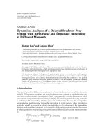
Figure 1: Representation of the genome for the placement of the
base station.
3.1. Representation
Figure 1 illustrates the representation of the genomes. A
genome is denoted as a vector g
= (c
1
, , c
k
), where c
k
=
(x
k
, y
k
) is the chromosome for the kth base station position.
This method fulfills (i) and (ii). K is the maximum number
of base stations, and all of these can be located in the x-range
[
−X

max
, X
max
]andy-range [−Y
max
, Y
max
] with origin (0, 0).
If the position of a base station is not defined, it is
expressed as NULL. This method applies for a case in which
there are fewer base stations than in K, so that it fulfills (i).
n(g) is defined as the number of EXISTENCE in g.Inorder
to satisfy (iii) and (iv), x
k
and y
k
must be real numbers. M is
assumed as population size.
3.2. Genetic operators (crossover and mutation)
It is necessary to design an initialization and a termination
method, a crossover and mutation operator, and a selection
strategy in order to define the reproduction procedure.
A proper initial population can provide a fast conver-
gence to the optimum point. It is desirable for a user to
define initial positions of base stations intuitively. The first
individual, c
1k
= (x
1k
, y

1k
)fork = 1, , K, is determined
by a user and other individuals (for m
= 2, , M)are
determined by the following rule: if c
1k
= NULL, then
c
mk
= NULL with probability P
I
n
or c
mk
= (υ
1
, υ
2
)
with probability 1
− P
I
n
,whereυ
1
= U(−X
max
, X
max
)and

υ
2
= U(−Y
max
, Y
max
). If c
1k
is defined (c
1k
/
= NULL), then
c
mk
= NULL with probability 1 − P
I
v
or c
mk
= (x
1k
+
ξ
1
, y
1k
+ ξ
2k
)withprobabilityP
I

v
,whereξ
1
, ξ
2
= N(0,σ
2
S
).
U(a, b) is a uniformly distributed random variable between
a and b. N(
x, σ
2
) denotes a Gaussian distributed random
variable with mean
x and variance σ
2
. P
I
n
and P
I
v
indicate
the probability of producing NULL from NULL and that
Dad
Mom
Child
Is Null
Is Null

Are Null
Are not Null
Null
123
···
K
123
···
K
3
3
3
3
3
3
&
&
3
3
3
Figure 2: One child crossover operation.
of producing EXISTENCE from EXISTENCE, respectively.
However, it may require further trials in order to determine
the global optimum if the initial value, as user defined, is
close to the local optimum. When the user does not define
any initial positions, it is decided that c
mk
= NULL with

P

I
n
or c
mk
= (υ
1
, υ
2
) with probability 1 −

P
I
n
for m = 1, , M,
where

P
I
n
denotes the probability of producing NULL.
A termination criterion is used to determine whether or
not a GA is finished. Generation, convergence, or population
convergence can terminate the procedure of genetic algo-
rithm. The easiest scheme is termination upon generation.
When the number of current generations is larger than the
specified number of generations, the algorithm is finished.
Termination upon convergence compares the previous best-
of-generation to the current best-of-generation. If the cur-
rent convergence is less than the requested convergence,
the reproduction procedure is ceased. Termination upon

population convergence compares the population average to
the score of the best individual in the population.
In the proposed application, one child crossover operator
is used. A single child c
child
k
is born from its father and mother,
c
dad
k
and c
mom
k
. Figure 2 shows the procedure of one child
crossover operation in the proposed algorithm. If one of
the parents is NULL, the child receives the other parent’s
attributes. Otherwise, the child is generated by (1), where σ
C
is the parameter of the crossover operation. |x
dad
k
− x
mom
k
|
and |y
dad
k
− y
mom

k
| can be used as a measure of closeness. This
method is based on the fact that if the attributions of both
parents are similar, the child’s attributions are also similar to
its parents.
Mutation is performed chromosome by chromosome
with probability P
mut
. Figure 3 shows the procedure of
the mutation operation in the proposed algorithm. The
mutation is very close to the initialization scheme with the
user-defined base station position. If c
mk
= NULL, redefine
4 EURASIP Journal on Wireless Communications and Networking
Individual 1
123
···
K
Individual 2
123
···
K
Individual m
123
···
K
Individual M 123
···
K

3
3
Null
(x, y)
3
3
Null
(x

, y

)
.
.
.
.
.
.
.
.
.
.
.
.
P
= P
n
P = 1 − P
n
P = 1 − P

v
P = P
v
Mutate with probability P
m
Figure 3: Mutation operation.
Tr afficmap Map
Propagation
model
Capacity
number of
BSs
FitnessEvaluator
Objective
function
Individual
(genome)
Figure 4: Fitness evaluation.
c
mk
= NULL with probability P
n
or c
mk
= (υ
1
, υ
2
)with
probability 1

− P
n
.Ifc
mk
/
= NULL, redefine c
mk
= (x
mk
+
χ
1
, y
mk
+ χ
2
)withprobabilityP
v
or c
mk
= NULL with
probability 1
− P
v
,whereχ
1
and χ
2
are Gaussian distributed
random variables with zero mean and variance σ

2
m
. P
mut
and
σ
2
m
are the parameters of the mutation operation.
A roulette wheel method is applied for the selection
scheme. This selection method chooses an individual based
on the magnitude of the fitness score relative to the rest
of the population. The higher the score, the more selective
an individual will be. Any individual has a probability p of
the choice, where p is equal to the fitness of the individual
divided by the sum of the fitness of each individual in the
population. Therefore, the individual with a high fitness level
can survive with high probability:
x
child
k
=
x
dad
k
+ x
mom
k
2
+ ζ

1
,
ζ
1
= N

0,

(x
dad
k
− x
mom
k
)σ
C
2

2

,
y
child
k
=
y
dad
k
+ y
mom

k
2
+ ζ
2
,
ζ
2
= N

0,

(y
dad
k
− y
mom
k
)σ
C
2

2

.
(1)
3.3. Fitness evaluation
Figure 4 illustrates the fitness evaluation procedure com-
posedofanevaluatorandanobjectivefunction.The
evaluator calculates the covered traffic by using a propagation
model, traffic map, and map for a path loss prediction. Cell

area covered by the base stations is evaluated, and the covered
traffic is then obtained. Considering coverage, power, and
economy efficiency, the objective function is defined as
f (G)
= ω
t
· f
t
(G)+ω
p
· f
p
(G)+ω
e
· f
e
(G), (2)
where f
t
, f
p
,and f
e
are the objective functions for coverage,
power, and economy respectively, and these are defined as:
f
t
(G) = traffic coverage rate
=
covered traffic

total traffic
,
f
p
(G) = BS power fitness
=
Available Maximum BS power − Used BS power
Available Maximum BS power
,
f
e
(G) = economic fitness
=
Available Maximum BSs − Used BSs
Available Maximum BSs
.
(3)
As the covered traffic area widens corresponding to the
given propagation model, f
t
(G) increases. Conversely, f
e
(G)
increases when fewer base stations are placed. Total fitness
is calculated with w
t
, w
p
,andw
e

subject to w
t
+ w
p
+
w
e
= 1. The weights are determined by the user’s preference.
If coverage is more important, then one may choose a
large w
t
. Otherwise, a large w
e
may be chosen to be more
desirable using fewer base stations. Therefore, the purpose
of optimization in this paper is to determine the maximum
traffic coverage with the minimum number of base stations
and minimum amount of power.
This paper uses Hata’s model to obtain the coverage of
the base station. It is possible that each individual can have K
(the maximum number of base stations). To achieve the cell
coverage, it is necessary to compute the path loss K times.
If the population is large, the computing power required
becomes very large. In this paper, to reduce processing time,
Hata’s model was used, which is fast for computing the path
loss with height information.
3.4. Scaling
After the fitness is decided, this value is not directly applied
for selection. The appropriate function is used to adjust the
fitness value. This function is termed “scaling” and there are

three general scaling methods.
The new fitness value f

is defined in Ta ble 1.
3.5. Selection
The purpose of the selection is to emphasize the fit individ-
uals in the population with the hopes that their offspring
will in turn have an even higher fitness value. Selection has
Yong Seouk Choi et al. 5
Table 1: Scaling methods.
Scaling model General form
Linear scaling f

= a· f + b
Sigma scaling f

= f − ( f − c·σ)
Power law scaling f

= f
k
2.5km
Figure 5: Homogenous traffic density for verification.
to be controlled in balance with crossover and mutation.
Too strong a selection signifies that suboptimal highly fit
individuals will take over the population, reducing the
diversity needed for further change and progress. Too weak
a selection will result in too slow an evolution. In this paper,
the common selection method of tournament selection, rank
selection, roulette-wheel selection, and uniform selection

were employed.
4. TESTIFY ALGORITHM
To test the proposed algorithm, a one-tiered hexagonal cel-
lular environment is considered, where traffic is distributed
uniformly in each hexagonal cell whose radius is 2.5 km. In
this case, the optimum position of the base station is in the
center of hexagon, and the optimum number of base stations
is obviously seven. A path loss prediction is carried out using
the equation L
= L
0
× (d/d
0
)
−4
,whereL
0
= 140 dB and
d
0
= 2.5 km. As the generation increases, the base stations
tend to be placed where they are optimum, and the number
of base stations is also converged automatically. After the
1000th generation, a base station placement that guarantees
99.78% coverage can be determined.
The input parameter for the proposed algorithm is listed
in Tabl e 2 . The maximum number of base stations depends
on the width of the target area. The wider the target area,
the more likely a greater amount of computing time for
convergence is needed. Population size is the solution set. If

the population size is large, the convergence of the solution
can be quicker. However, in this case the total computing
time is larger, as a processing of the propagation model will
be needed for each individual in the population. As the
individuals with low fitness values are removed, the initial
values of base station’s maximum number and location are
not related to the entire performance. Therefore, a null-to-
null probability and pos-to-pos probability is loosely coupled
Variable mutation probability (tournament selection)
0 100 200 300 400 500 600 700 800 900 1000
Generations
0.3
0.4
0.5
0.6
0.7
0.8
0.9
1
Scores
p
mut
= 0.1
p
mut
= 0.2
p
mut
= 0.05
p

mut
= 0.15
p
mut
= 0.01
Figure 6: Fitness in various mutation probabilities.
Va ri ab le m ut at i on s td
0 100 200 300 400 500 600 700 800 900 1000
Generations
0.65
0.7
0.75
0.8
0.85
0.9
0.95
1
Scores
99%
95%
90%
70%
60%
80%
Figure 7: Fitness in various mutation deviations.
with the fitness relationship, and the mutation probability in
a real value representation is the main factor in speeding the
convergence.
Fitness with various mutation probabilities in each
generation is shown in Figure 6. The higher the mutation

probability, the better the fitness. However, too high a
mutation probability has a tendency to downgrade the per-
formance, as it has a frequently changing possible solutions
set. In the given homogenous trafficinFigure 5, it is known
that the best performance is shown when the mutation
probability is 0.1 (Figure 6).
Figure 7 shows that a high deviation of mutation will be
good for performance. From Figures 8 to 10, the changing of
fitness with various scaling methods becomes clear.
6 EURASIP Journal on Wireless Communications and Networking
Table 2: Input parameters list.
Parameter Basic value Range
The maximum number of BS Depend on width of area Variable
Population size 20 Variable
Crossover probability 1.0 Variable
Mutation probability 0.1 Variable
Init null-to-null probability 0.2 Variable
Init pos-to-pos probability 0.95 Variable
Null-to-null probability 0.5 Variable
Pos-to-pos probability 0.5 Variable
Standard deviation in mutation 3062.2 (95% in 6 Km) Variable
Minimum BS power 20 dBm Variable
Maximum BS power 40 dBm Variable
Allowable traffic per BS 50 Erlang Variable
Receiver sensitivity
−80 dBm Variable
Selection Tournament Roulette wheel, rank, tournament, uniform
Scaling No scaling No scale, linear, power law, sigma truncation
Variable linear scaling multiplier, c (roulette selection)
0 100 200 300 400 500 600 700 800 900 1000

Generations
0.65
0.7
0.75
0.8
0.85
0.9
0.95
1
Scores
No scaling
c
= 1.5
c
= 2
c
= 2.5
c
= 3
Figure 8: Fitness with linear scaling.
Selection is the operation by which chromosomes are
selected for the reproduction of the next generation. The
function of selection is that chromosomes corresponding to
individuals with a higher fitness have a higher probability
of being selected. There are a number of possible selection
schemes. In this paper, several selection schemes were
verified as mentioned in Chapter 3.5. Good results cannot
be expected with the selections that do not have balanced
crossover and mutation.
In Figure 11, it is clear that the fitness changes with the

selection schemes, and the result shows the fitness order;
tournament selection > rank selection > roulette-wheel
selection > uniform selection.
Variable power scaling factor, k (roulette selection)
0 100 200 300 400 500 600 700 800 900 1000
Generations
0.65
0.7
0.75
0.8
0.85
0.9
0.95
1
Scores
No scaling
k
= 1.5
k
= 2
k
= 2.5
k
= 3
k
= 3.5
Figure 9: Fitness with power law scaling.
Figures 12 to 16 show the optimization processing of base
station displacements. Figure 12 shows the initial random
location of the base stations, and in this case five base stations

have covered 69% of the target area. In Figure 13,seven
base stations have covered 92% of target area with uniform
selection, but it is still not optimized. Figure 14 is the result of
a roulette-wheel selection, and this is an improvement over
the uniform selection. It covers 93.85% of the target area.
The rank selection covers 97.90%; this is a very good result.
The tournament selection offers 99.78% coverage. This is
approximately at the optimization level. As fitness is sensitive
in terms of selection schemes, optimization processing needs
appropriate selection schemes.
Yong Seouk Choi et al. 7
Variable sigma truncation multiplier, c (roulette selection)
0 100 200 300 400 500 600 700 800 900 1000
Generations
0.65
0.7
0.75
0.8
0.85
0.9
0.95
1
Scores
No scale
c
= 2
c
= 3
c
= 4

c
= 5
Figure 10: Fitness with sigma truncation.
Variable selection scheme
0 100 200 300 400 500 600 700 800 900 1000
Generations
0.65
0.7
0.75
0.8
0.85
0.9
0.95
1
Scores
Tournament
Rank
Roulette wheel
Uniform
Figure 11: Fitness with selection schemes.
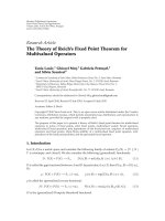
5. SIMULATION RESULTS
To demonstrate if the proposed algorithm determines
which positions match optimum location, a simulation was
conducted on areas similar to that in Figures 17 and 18
(inhomogeneous traffic). The actual-valued representations
in this paper, as mentioned above, consist of the candidate
location of the base station’s transmit power. Figure 17 shows
the altitude map of the target areas, and Figure 18 shows the
trafficdensitymap.Thetraffic density is inhomogeneous and
the target area for simulation is an urban pattern. The width

of the area for simulation is 12 Km
× 12 Km and the size
of the bin is 120 m
× 120 m. Therefore, the total number of
Initial BS-placement (69% coverage)
−10 −8 −6 −4 −20 2 4 6 8
×10
3
X
−6
−4
−2
0
2
4
6
×10
3
Y
Figure 12: Initial base station location.
BS-placement after 1000 generations (uniform),
91.99% coverage
−8 −6 −4 −20 2 4 6 8
×10
3
X
−6
−4
−2
0

2
4
6
×10
3
Y
Figure 13: After the 1000th generation, base station location with
uniform selection.
bins is 10 000. The parameters for the simulation are listed in
Ta ble 3.
Figures 19 and 20 show the location of the base
station from one generation to 500 generations, when the
weighting condition of their object function is (ω
t
, ω
p
, ω
e
) =
(0.9, 0.0, 0.1). The assigned transmit power range of each
base station is from 22.63 dBm to 33.84 dBm, and its mean
value is 33.84 dBm. In this case, the coverage rate is 82.62%
and the fitness value is 0.74258.
In the case where the condition of object function is
(ω
t
, ω
p
, ω
e

) = (0.8, 0.1,0.1), the results are shown in Figures
21 and 22. The coverage rate is 77.47%, and the fitness
value is 0.663181. The assigned transmit power range of
each base station is from 211 752 dBm to 3 857 794 dBm,
and its mean value is 323 230 dBm. As the trafficcapacity
is limited, the cell boundaries of the high-traffic density are
8 EURASIP Journal on Wireless Communications and Networking
Table 3: Simulation parameters.
Population size 30 Maximum BS power 40 dBm
Mutation probability 0.2 Receiver sensitivity
−85 dBm
Mutation std. 3062.2 Allowable trafficperBS 50Erlang
Init null-to-null probability 0.2 Selection scheme Tournament
Init pos-to-pos probability 0.95 Scaling scheme No scaling
null-to-null probability 0.5 Termination criterion Generation
Pos-to-pos probability 0.5 Eliticism Used
Minimum BS power 20 dBm Propagation model Hata model (SU)
BS-placement after 1000 generation (roulette wheel),
93.85% coverage
−8 −6 −4 −20 2 4 6 8
×10
3
X
−6
−4
−2
0
2
4
6

×10
3
Y
Figure 14: After the 1000th generation, base station location with
roulette-wheel selection.
BS-placement after 1000 generations (rank),
97.9% coverage
−8 −6 −4 −20 2 4 6 8
×10
3
X
−6
−4
−2
0
2
4
6
×10
3
Y
Figure 15: After the 1000th generation, base station location with
rank selection.
BS-placement after 1000 generations (tournament),
99.78% coverage
−8 −6 −4 −20 2 4 6 8
×10
3
X
−6

−4
−2
0
2
4
6
×10
3
Y
Figure 16: After the 1000th generation, base station location with
tournament selection.
−6000 0 6000
−6
0
6
×10
3
0
50
100
150
200
250
300
350
400
Figure 17: Altitude map.
less than those of the low-traffic density. The coverage rate
is decreased according to the changing weight of the traffic
factor, from 0.9 to 0.8. As the weight of the power factor

increases, the actual assigned transmit power value decreases.
Yong Seouk Choi et al. 9
Tr affic map in Erlang
−6 −4 −20 2 4 6
×10
3
X
−6
−4
−2
0
2
4
6
×10
3
Y
0.05
0.1
0.15
0.2
0.25
0.3
0.35
0.4
Figure 18: Trafficdensitymap.
32.4489
36.9757
35.3866
34.3922

29.4681
37.7027
31.957
35.2997
28.1567
33.2694
32.695
22.6272
35.2396
32.9508
32.8581
39.3609
38.768
37.7642
36.1991
33.2659
Tr affic map in Erlang
−6 −4 −20 2 4 6
×10
3
X
−6
−4
−2
0
2
4
6
×10
3

Y
0.05
0.1
0.15
0.2
0.25
0.3
0.35
0.4
Figure 19: After 500 generations, the location of the base stations,
(ω
t
, ω
p
, ω
e
) = (0.9,0.0, 0.1).
In the results shown in Figure 21, the overlapped base station
is clearly shown. The cause of this is the decrease of the
weighted economy factor. The traffic map that was used for
the simulation consisted of high-trafficdensityareasand
very low-traffic density areas such as mountains and rivers.
Therefore, traffic is scattered in all directions on the map;
consequently, the search space becomes larger. To obtain a
better coverage rate, the population size can be enlarged or
the mutation probability can be increased. Additionally, it is
necessary to process more generations.
6. CONCLUSION
In this paper, given inhomogeneous traffic information and
the map for the propagation model, a new algorithm was

proposed that enables the optimization of the locations
0 50 100 150 200 250 300 350 400 450 500
Generation
0
0.1
0.2
0.3
0.4
0.5
0.6
0.7
0.8
0.9
Scores
Coverage rate
To t a l fi t n e s s
Power fitness
Economy fitness
Figure 20: Fitness value, (ω
t
, ω
p
, ω
e
) = (0.9,0.0, 0.1).
34.1883
30.5128
37.228
31.6579
33.3518

38.5779
30.3895
28.272
37.0711
34.6587
31.9989
32.7122
26.7958
26.9319
35.1755
37.4056
21.1752
29.5987
36.4352
Tr affic map in Erlang
−6 −4 −20 2 4 6
×10
3
X
−6
−4
−2
0
2
4
6
×10
3
Y
0.05

0.1
0.15
0.2
0.25
0.3
0.35
0.4
Figure 21: After 500 generations, the location of the base stations,
(ω
t
, ω
p
, ω
e
) = (0.8,0.1, 0.1).
0 50 100 150 200 250 300 350 400 450 500
Generation
0
0.1
0.2
0.3
0.4
0.5
0.6
0.7
0.8
Score
Coverage rate
To t a l fit n e s s
Power fitness

Economy fitness
Figure 22: Fitness values, (ω
t
, ω
p
, ω
e
) = (0.8,0.1, 0.1).
10 EURASIP Journal on Wireless Communications and Networking
and transmitted power of a base station. In addition, this
algorithm includes an economic factor (the number of base
stations). Good use was made of the genetic algorithm and, it
was excellent for obtaining a solution of complex problems.
Genetic operators using the real-valued representation are
also suggested, and the objective function is defined in
consideration of the coverage, the transmitted power of base
station and the economy efficiency through an adjustment
of crossover and mutation. The selection, input parameters,
and scaling are shown to be tightly coupled with the algo-
rithm performance. Therefore, there is a need for these to be
harmonized. From a simulation, the proposed algorithm was
verified.
REFERENCES
[1] J. R. Evans and E. Minieka, Optimization Algorithms for
Networks and Graphs, Marcel Dekker, New York, NY, USA,
1992.
[2] P. Calegari, F. Guidec, P. Kuonen, and D. Wagner, “Genetic
approach to radio network optimization for mobile systems,”
in Proceedings of the 47th IEEE Vehicular Technolog y Conference
(VTC ’97), vol. 2, pp. 755–759, Phoenix, Ariz, USA, May 1997.

[3] X. Huang, U. Behr, and W. Wiesbeck, “Automatic base station
placement and dimensioning for mobile network planning,” in
Proceedings of the 52nd IEEE Vehicular Technology Conference
(VTC ’00), vol. 4, pp. 1544–1549, Boston, Mass, USA, Septem-
ber 2000.
[4] J. H. Holland, Adaptation in Natural and Artificial Systems,
University of Michigan Press, Ann Arbor, Mich, USA, 1975.