Báo cáo hóa học: " Research Article Multisource Images Analysis Using Collaborative Clustering" potx
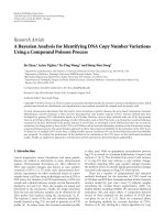
Bạn đang xem bản rút gọn của tài liệu. Xem và tải ngay bản đầy đủ của tài liệu tại đây (8.31 MB, 11 trang )
Hindawi Publishing Corporation
EURASIP Journal on Advances in Signal Processing
Volume 2008, Article ID 374095, 11 pages
doi:10.1155/2008/374095
Research Article
Multisource Images Analysis Using Collaborative Clustering
Germain Forestier, C
´
edric Wemmert, and Pierre Ganc¸arski
LSIIT, UMR 7005 CNRS/ULP, University Louis Pasteur, 67070 Strasbourg Cedex, France
Correspondence should be addressed to Germain Forestier,
Received 1 October 2007; Revised 20 February 2008; Accepted 26 February 2008
Recommended by C. Charrier
The development of very high-resolution (VHR) satellite imagery has produced a huge amount of data. The multiplication of
satellites which embed different types of sensors provides a lot of heterogeneous images. Consequently, the image analyst has
often many different images available, representing the same area of the Earth surface. These images can be from different dates,
produced by different sensors, or even at different resolutions. The lack of machine learning tools using all these representations
in an overall process constraints to a sequential analysis of these various images. In order to use all the information available
simultaneously, we propose a framework where different algorithms can use different views of the scene. Each one works on
adifferent remotely sensed image and, thus, produces different and useful information. These algorithms work together in a
collaborative way through an automatic and mutual refinement of their results, so that all the results have almost the same
number of clusters, which are statistically similar. Finally, a unique result is produced, representing a consensus among the
information obtained by each clustering method on its own image. The unified result and the complementarity of the single
results (i.e., the agreement between the clustering methods as well as the disagreement) lead to a better understanding of the scene.
The experiments carried out on multispectral remote sensing images have shown that this method is efficient to extract relevant
information and to improve the scene understanding.
Copyright © 2008 Germain Forestier et al. This is an open access article distributed under the Creative Commons Attribution
License, which permits unrestricted use, distribution, and reproduction in any medium, provided the original work is properly
cited.
1. INTRODUCTION
Unsupervised classification, also called clustering, is a well-
known machine learning tool which extracts knowledge
from datasets [1, 2]. The purpose of clustering is to group
similar objects into subsets (called clusters), maximizing
the intracluster similarity and the intercluster dissimilarity.
Many clustering algorithms have been developed during the
last 40 years,each one is based on a different strategy. In
image processing, clustering algorithms are usually used by
considering the pixels of the image as data objects: each pixel
is assigned to a cluster by the clustering algorithm. Then, a
map is produced, representing each pixel with the colour of
the cluster it has been assigned to. This cluster map, depicting
the spatial distribution of the clusters, is then interpreted
by the expert who assigns to each cluster (i.e., colour in
the image) a mean in terms of thematic classes (vegetation,
water, etc.).
In contrast to the supervised classification, unsupervised
classification requires very few inputs. The classification
process only uses spectral properties to group pixels together.
However, it requires a precise parametrization by the user
because the classification is performed without any control.
Other potential problems exist, especially when the user
attempts to assign a thematic class to each produced cluster.
On the one hand, some thematic classes may be represented
by a mix of different types of surface covers: a single thematic
class may be split among two or more clusters (e.g., a park
is often an aggregate of vegetation, sand, water, etc.). On
the other hand, some of the clusters may be meaningless, as
they include too many mixed pixels: a mixed pixel (mixel)
represents the average energy reflected by several types of
surface present within the studied area.
These problems have increased with the recent availabil-
ity of very high-resolution satellite sensors, which provide
many details of the land cover. Moreover, several images
with different characteristics are often available for the same
area: different dates, from different kinds of remote sensing
acquisition systems (i.e., with different numbers of sensors
and wavelengths) or different resolutions (i.e., different sizes
2 EURASIP Journal on Advances in Signal Processing
of surface of the area that a pixel represents on the ground).
Consequently, the expert is confronted to a too great mass
of data: the use of classical knowledge extraction techniques
became too complex. It needs specific tools to extract
efficiently the knowledge stored in each of the available
images.
To avoid the independent analysis of each image, we
propose to use different clustering methods, each working on
adifferent image of the same area. These different clustering
methods collaborate together during a refinement step of
their results, to converge towards a similar result. At the
end of this collaborative process, the different results are
combined using a voting algorithm. This unified result rep-
resents a consensus among all the knowledge extracted from
the different sources. Furthermore, the voting algorithm
highlights the agreement and the disagreement between the
clustering methods. These two pieces of information, as well
as the result produced by each clustering method, lead to a
better understanding of the scene by the expert.
The paper is organized as follows. First, an overview
of multisource applications is introduced in Section 2.The
collaborative method to combine different clustering algo-
rithms is then presented in Section 3. Section 4 presents in
details the paradigm of multisource images and the different
ways to use it in the collaborative system. Section 5 shows
an experimental evaluation of the developed methods, and
finally, conclusions are drawn in Section 6.
2. MULTISOURCE IMAGES ANALYSIS
In the domain of Earth observation, many works focus on
the development of data-fusion techniques to take advantage
of all the available data on the studied area. As discussed in
[3], multisource image analysis can be achieved at different
levels, according to the stage where the fusion takes place:
pixel, feature, or decision level.
At pixel level, data fusion consists in creating a fused
image based on the sensors measurements by merging the
values given by the various sources. A method is proposed
in [4] for combining multispectral, panchromatic, and radar
images by using conjointly the intensity-hue-saturation
transform and the redundant wavelet decomposition. In [5],
the authors propose a multisource data-fusion mechanism
using generalized positive Boolean functions which consists
of two steps: a band generation is carried out followed
by a classification using a positive Boolean function-based
classifier. In the case of feature fusion, the first step creates
new features from the various datasets; these new features
are merged and analyzed in a second step. For example,
a segmentation can be performed on the different image
sources and these segmentations are fused [6]. In [7], the
authors present another method based on the Dempster-
Shafer theory of evidence and using the fuzzy statistical
estimation maximization (FSEM) algorithm to find an
optimal estimation of the inaccuracy and uncertainty of the
classification.
The fusion of decisions consists in finding a single deci-
sion (also called consensus) from all the decisions produced
by the classifiers. In [8], the authors propose a method based
on the combination of neural networks for multisource
classification. The system exposed in [9] is composed of
an ensemble of classifiers trained in a supervised way on
a specific image, and can be retrained in an unsupervised
way to be able to classify a new image. In [10], a general
framework is presented for combining information from
several supervised classifiers using a fuzzy decision rule.
In our work, we focus on fusion of decisions from
unsupervised classifications, each one produced from a
different image. Contrary to the methods presented above,
we propose a mechanism which finds a consensus according
to the decisions taken by each of the unsupervised classifier.
3. COLLABORATIVE CLUSTERING
Many works focus on combining different results of clus-
tering, which is commonly called clustering aggregation
[11], multiple clusterings [12], or cluster ensembles [
13, 14].
All these approaches try to combine different results of
clustering in a final step. In fact, these results must have
the same number of clusters (vote-based methods) [14]or
the expected clusters must be separable in the data space
(coassociation-based methods) [12]. This latter property is
almost never encountered in remote sensing image analysis.
It is difficult to compute a consensual result from cluster-
ing results with different numbers of classes or different
structures (flat partitioning or hierarchical result) because of
the lack of a trivial correspondence between the clusters of
these different results. To address the problem, we present in
this section a framework where different clustering methods
work together in a collaborative way to find an agreement
about their proposals. This collaborative process consists in
an automatic and mutual refinement of the clustering results,
until all the results have almost the same number of clusters,
and all the clusters are statistically similar. At the end of
this process, as the results have comparable structures, it is
possible to define a correspondence function between the
clusters, and to apply a unifying technique such as a voting
method [15].
Before the description of the collaborative method, we
introduce the correspondence function used within it.
3.1. Intercluster correspondence function
There is no problem to associate classes of different super-
vised classifications as a common set of class labels is
given for all the classifications. Unfortunately, in the case of
unsupervised classifications, the results may not have a same
number of clusters, and no information is available about the
correspondence between the different clusters of the different
results.
To address the problem, we have defined a new interclus-
ter correspondence function, which associates to each cluster
from a result, a cluster from each of the other results.
Let
{R
i
}
1≤i≤m
be the set of results given by the different
algorithms. Let
{C
i
k
}
1≤k≤n
i
be the clusters of the result R
i
.
Figure 1 shows an example of such results.
Germain Forestier et al. 3
C
1
1
C
1
2
C
1
3
C
1
4
C
2
1
C
2
2
C
2
3
C
2
4
C
2
5
C
2
6
Figure 1: Two clustering results of the same data but using a
different method.
The corresponding cluster CC(C
i
k
, R
j
)ofaclusterC
i
k
from
R
i
in the result R
j
, i
/
= j, is the cluster from R
j
which is the
most similar to C
i
k
:
CC
C
i
k
, R
j
=
C
j
with S
C
i
k
, C
j
=
max
S
C
i
k
, C
j
l
, ∀l ∈[1, n
j
]
,
(1)
where S is the intercluster similarity which evaluates the
similarity between two clusters of two different results.
It is calculated from the recovery of the clusters in two
steps. First, the intersection between each couple of clusters
(C
i
k
, C
j
l
), from two different results R
i
and R
j
, is calculated
and written in the confusion matrix M
i,j
:
M
i,j
=
⎛
⎜
⎜
⎜
⎝
α
i,j
1,1
··· α
i,j
1,n
j
.
.
.
.
.
.
.
.
.
α
i,j
n
i
,1
··· α
i,j
n
i
,n
j
⎞
⎟
⎟
⎟
⎠
,whereα
i,j
k,l
=
|
C
i
k
C
j
l
|
C
i
k
.
(2)
Then, the similarity S(C
i
k
, C
j
l
) between two clusters C
i
k
and C
j
l
is evaluated by observing the relationship between
the size of their intersection and the size of the cluster itself,
and by taking into account the distribution of the data in the
other clusters as follows:
S
C
i
k
, C
j
l
=
α
i,j
k,l
α
j,i
l,k
. (3)
Figure 2 presents the correspondence function obtained
by using the intercluster similarity on the results shown in
Figure 1.
3.2. Collaborative process overview
The entire clustering process is broken down in three main
following phases:
(i) initial clusterings: each clustering method computes a
clustering of the data using its parameters;
(ii) results refinement: a phase of convergence of the results,
which consists of conflicts evaluation and resolution,
is iterated as long as the quality of the results and their
similarity increase;
(iii) Unification: the refined results are unified using a
voting algorithm.
C
1
1
C
1
2
C
1
3
C
1
4
C
2
1
C
2
2
C
2
3
C
2
4
C
2
5
C
2
6
Figure 2: The correspondence between the clusters of the two
results from Figure 1 using the intercluster similarity by recovery.
3.2.1. Initial clusterings
During the first step, each clustering method is initialized
with its own parameters and a clustering is performed on
a remotely sensed image: all the pixels are grouped into
different clusters.
3.2.2. Results refinement
The mechanism we propose for refining the results is based
on the concept of distributed local resolution of conflicts, by
the iteration of four phases:
(i) detection of the conflicts by evaluating the dissimilari-
ties between couples of results;
(ii) choice of the conflicts to solve;
(iii) local resolution of these conflicts;
(iv) management of the local modifications in the global
result (if they are relevant).
(a) Conflicts detection
The detection of the conflicts consists in seeking all the
couples (C
i
k
, R
j
), i
/
= j,suchasC
i
k
/
= CC(C
i
k
, R
j
). One
conflict K
i,j
k
is identified by one cluster C
i
k
and one result
R
j
.
We associate to each conflict a measurement of its
importance, the conflict importance coe fficient, calculated
according to the intercluster similarity
CI
K
i,j
k
=
1 −S
C
i
k
, CC
C
i
k
, R
j
. (4)
(b) Choice of the conflicts to solve
During an iteration of refinement of the results, several local
resolutions are performed in parallel. A conflict is selected in
the set of existing conflicts and its resolution is started. This
conflict, like all those concerning the two results involved in
the conflict, are removed from the list of the conflicts. This
process is iterated, until the list of the conflicts is empty.
Different heuristics can be used to choose the conflict to
solve, according to the conflict importance coefficient (4). We
choose to try to solve the most important conflict first.
4 EURASIP Journal on Advances in Signal Processing
let n =|CCs(C
i
k
, R
j
)|
let R
i
(resp., R
j
) be the result of the application of an
operator on R
i
(resp., R
j
)
if n>1 then
R
i
= R
i
\{C
i
k
}∪{split(C
i
k
, n)}
R
j
= R
j
\CCs(C
i
k
, R
j
) ∪{merge(CCs(C
i
k
, R
j
))}
else
R
i
= reclustering(R
i
, C
i
k
)
end if
Algorithm 1
(c) Local resolution of a conflict
The local resolution of a conflict K
i,j
k
consists of applying an
operator on each result involved in the conflict, R
i
and R
j
,
to try to make them more similar.
The operators that can be applied to a result are the
following:
(i) merging of clusters: some clusters are merged together
(all the objects are merged in a new cluster that
replaces the clusters merged),
(ii) splitting of a cluster in subclusters: a clustering is
applied to the objects of a cluster to produce subclus-
ters,
(iii) reclustering of a group of objects: one cluster is
removed and its objects are reclassified in all the other
existing clusters.
The operator to apply is chosen according to the corre-
sponding clusters of the cluster involved in the conflict. The
corresponding clusters (CCs) of a cluster are an extension of
the definition of the corresponding cluster (1):
CCs
C
i
k
, R
j
=
C
j
l
| S
C
i
k
, C
j
l
>p
cr
, ∀l ∈[1, n
j
]
,
(5)
where p
cr
,0≤ p
cr
≤ 1, is given by the user. Having found the
corresponding clusters of the cluster involved in the conflict,
an operator is chosen and applied as shown in Algorithm.
But the application of the two operators is not always
relevant. Indeed, it does not always increase the similarity of
the results implied in the conflict treated, and especially, the
iteration of conflict resolutions may lead to a trivial solution
where all the methods are in agreement. For example, they
can converge towards a result with only one cluster including
all the objects to classify, or towards a result having one
cluster for each object. These two solutions are not relevant
and must be avoided.
So we defined a criterion γ, called local similarity crite-
rion, to evaluate the similarity between two results, based
on the intercluster similarity S (3) and a quality criterion δ
(given by the user):
γ
i,j
=
1
2
p
s
·
1
n
i
n
i
k=1
ω
i,j
k
+
1
n
j
n
j
k=1
ω
j,i
k
+ p
q
·
δ
i
+ δ
j
,
(6)
where
ω
i,j
k
=
n
j
l=1
S
C
i
k
,CC
C
i
k
, R
j
(7)
and, p
q
and p
s
are given by the user (p
q
+ p
s
= 1). The quality
criterion δ
i
represents the internal quality of a result R
i
(the
compactness of its clusters, e.g.).
At the end of each conflict resolution, the local similarity
criterion enables to choose which couple of results are to be
kept: the two new results, the two old results, or one new
result with one old result.
(d) Global management of the local modifications
After the resolutions of all these local conflicts, a global
application of the modifications proposed by the refinement
step is decided if it improves the quality of the global result.
The global agreement coefficient of the results is evaluated
according to all the local similarity between each couple of
results. It evaluates the global similarity of the results and
their quality:
Γ
=
1
m
m
i=1
Γ
i
,(8)
where
Γ
i
=
1
m −1
m
j=1
j
/
= i
γ
i,j
. (9)
Even if the local modifications decrease this global
agreement coefficient, the solution is accepted to avoid to fall
in a local maximum. If the coefficient is decreasing too much,
all the results are reinitialized to the best temporary solution
(the one with the best global agreement coefficient).
Theglobalprocessisiterateduntilsomeconflictscanbe
solved.
3.2.3. Unification
In the final step, all the results tend to have the same number
of clusters, which are increasingly similar. Thus, we use a vot-
ing algorithm [15] to compute a unified result combining the
different results. This multiview-voting algorithm enables
to combine in one unique result, many different clustering
results that have not necessarily the same number of clusters.
The basic idea is that for each object to cluster, each result
R
i
votes for the cluster it has found for this object, C
i
k
for
example, and for the corresponding cluster of C
i
k
in all the
other results. The maximum of these values indicates the best
cluster for the object, for example C
j
l
. This means that this
object should be in the cluster C
j
l
according to the opinion
of all the methods.
After having done the vote for all objects, a new cluster
is created for each best cluster found if a majority of the
methods has voted for this cluster. If not, the object is affected
to a special cluster, containing all the objects that do not
have the majority, which means they have been classified
differently in too many results.
Germain Forestier et al. 5
Real object O
V
1
V
n
.
.
.
D
1
D
n
E
1
1
={12; 45;234}
E
1
2
={2; 129;73}
.
.
.
E
1
N
1
={172; 29;89}
E
n
1
={172; 4;34; 98}
E
n
2
={27; 129;173; 53}
.
.
.
E
n
N
n
={12; 129;9; 255}
Figure 3: Different points of view V
1
to V
n
on a same object O (the
river) producing different descriptions D
1
to D
n
of the object.
4. MULTISOURCE IMAGE PARADIGM
The method described in the previous section can use
different types of clustering algorithms, but they work with
only one common dataset (i.e., the same image for each
clustering algorithm). In this section, we describe how we
make the collaborative method able to combine different
sources of data and to extract knowledge from them.
The problem can be described as follows. There exists
one real object O that can be viewed from different points
of view, and the goal is to find one description of this object,
according to all the different points of view (Figure 3). Each
view V
i
of the object is represented by a data set D
i
which is
composed of many elements
{E
i
1
, , E
i
N
i
}.EachelementE
i
k
is described by a set of attributes {(a
i,k
l
, v
i,k
l
)}
1<l<n
i,k
composed
of a name a and a value υ.
Three different cases can be happened (Figure 4):
(a) E
i
k
= E
j
k
for all i, j, a
i,k
l
= a
j,k
l
for all l and v
i,k
l
/
= v
j,k
l
(e.g., two remote sensing images of a same region,
from the same satellite, but at different seasons);
(b) E
i
k
= E
j
k
for all i, j and a
i,k
l
/
=a
j,k
l
(e.g., two remote sens-
ing images of a same region, having a same resolution,
butfromtwodifferent satellites with different sensors);
(c) E
i
k
/
= E
j
k
for all i, j | i
/
= j (e.g., two remote sensing
images of a same region, but having a different reso-
lution, and from two different satellites with different
sensors).
4.1. Multisource objects clustering
A first method to classify multisource objects is to merge
the attributes from the different sources. Each object has a
new description composed of the attributes of all the sources
(Figure 5(a)). But this technique may produce many clusters
because the description of the object would be too precise
(i.e., would have an important number of attributes). So
it is hard to discriminate the objects. Indeed, due to the
D
i
xs1 xs2 xs3
12 32 151
D
j
xs1 xs2 xs3
15 41 131
(a) Same resolution/same sensors/different dates: a pixel is described
by the same attributes but has different values because of its evolution
during the two dates
D
i
xs1 xs2 xs3
12 32 151
D
j
tm1 tm2 tm3 tm4
7 17 161 234
(b) Same resolutions/different sensors: a pixel is described by three
attributes in the image on the left, but by four attributes in the image
on the right
D
i
xs1 xs2 xs3
12 32 151
D
j
tm1 tm2 tm3 tm4
7 17 161 234
(c) Different resolutions/different sensors: the image D
i
has a higher
resolution than D
j
, the two images do not the same size and the pixels
arenomorethesame
Figure 4: The three different cases of image comparison.
curse of dimensionality [16], most of the classical distance-
based algorithms are not efficientenoughtoanalyseobjects
having many attributes, the distances between these objects
being not different enough to correctly determine the nearest
objects. In addition, the increase of the spectral dimension-
ality increases the problems like the Hughes phenomena [17]
which describes the harmful objects of high-dimensionality
objects.
A second way to combine all the attributes (Figure 5(b))
is to first classify the objects with each data sets. These
clusterings are made independently. Then a new description
of each object is built, using the number of each cluster found
by the first classifications. And finally a classification is made
using these new descriptions of the objects. The first phase
of clusterings enables to reduce the data space for the final
clustering, making it easier. This approach is similar to the
stacking method [18].
In our approach, the collaborative clustering (Figure
5(c)) is made quite as in the second method presented above.
Each data set is classified according to its attributes. Although
the clusterings are not made independently but they are
refined to make them converge towards a unique result. Then
6 EURASIP Journal on Advances in Signal Processing
Data D
1
··· Data D
N
Clustering Final result
(a) The different data are merged to produce a new dataset which is
classified
Data D
1
···
Data D
N
Clustering 1
Clustering N
···
Combination
Final result
(b) Each dataset is classified independently by a different clustering
method and the results are combined
Data D
1
···
Data D
N
Clustering 1
Clustering N
···
Combination
Final result
(c) Each dataset is classified by a different clustering method that
collaborates with the other methods and then the results are combined
Figure 5: Different data fusion techniques.
only they are unified by a voting method, or a clustering as
in method (b).
To integrate this new approach in our system, we affect
one dataset to each clustering method. All the process of
results refinement stay unchanged, but we are confronted
with the problem of the comparison of the different results,
and precisely of the estimation of the intercluster similarity
(see Section 3.1). In the two first cases presented above (same
elements with different descriptions), the confusion matrix
and the intercluster similarity defined in Section 3 can be
used. However, in the third case (different elements with
different descriptions), it cannot be applied because the
computation of a confusion matrix between two clusterings
involves that the clusters refer to the same objects. The
definition of a confusion matrix between datasets of different
objects is in the general case very hard, or even impossible.
Nevertheless, in some particular problems, it is possible to
define it. In the next section, we describe how this matrix
can be evaluated in the domain of multiscale remote sensing
images clustering.
4.2. Multiscale remote sensing images classification
In remote sensing image classification, the problem of the
image resolution is not easy to resolve. The resolution of an
image is the size covered by one pixel in the real world.For
example, the very high-resolution satellites give a resolution
of 2.5m, that is, one pixel is a square of 2.5 m
× 2.5m. One
can have different images of a same area but not with the
same resolution. So it is really difficult to use these different
images because they do not include the same objects to
cluster (Figure 6).
Reality
Clustering of low
resolution image
Clustering of high
resolution image
Figure 6: How can someone compare objects that are different but
that represent a same “real” object? A same reality is viewed at two
different resolutions. For example the river is composed of 17 pixels
on the low resolution image but it is composed of 43 pixels on the
high resolution image.
For example, satellites often produce two kinds of images
of the same area, a panchromatic and a multispectral. The
panchromatic has a good spatial resolution but a low spectral
resolution and, on the contrary, multispectral has a good
spectral resolution but a low spatial resolution. A solution
to use these two sources of information is to fuse the
panchromatic and the multispectral images in a unique one.
Many methods have been investigated in the last few years to
fuse these two kinds of images and to produce an image with
a good spectral and spatial resolution [19, 20].
A fused image can be used directly as input of our
collaborative system. However, the fused image could not be
available or the user would not like to use the fusion or would
prefer to process the images without fusing them. In these
cases, we have to modify our system to be able to support
images at different resolutions. The modification consists of
a new definition of the confusion matrix (see (2)) between
two clustering results.
In the previous definition given in Section 3, each line of
the confusion matrix is given by the confusion vector α
i,j
k
of
the cluster C
i
k
from the result R
i
compared to the n
j
clusters
found in the result R
j
:
α
i,j
k
=
α
i,j
k,l
l=1, ,n
j
,whereα
i,j
k,l
=
|
C
i
k
∩C
j
l
|
|C
i
k
|
. (10)
If the two results were not computed using the same data
and if the resolution of the two images are not the same, it
Germain Forestier et al. 7
is impossible to compute |C
i
k
∩ C
j
l
|.Soweproposeanew
definition of the confusion vector for a class C
i
k
from the
result R
i
compared to the result R
j
.
Definition 1 (new confusion matrix). let r
i
and r
j
be the
resolution of the two images I
i
and I
j
; let λ
I
1
,I
2
be a function
that associates each pixel of the image I
1
to one pixel of
the image I
1
,withr
1
≤ r
2
; let #(C, I
1
, I
2
) =|{p ∈ C :
cluster (λ
I
1
,I
2
(p)) = C}|; if r
i
≤ r
j
α
i,j
k,l
=
#
C
i
k
, I
i
, I
j
|C
i
k
|
(11)
else
α
i,j
k,l
=
#
C
j
l
, I
j
, I
i
|C
i
k
|
×
r
j
r
i
. (12)
With this new definition of the confusion matrix, the
results can be compared with each other and evaluated
as described previously. In the same way, the conflicts
resolution phase is unchanged.
Because the images have not the same resolution, it is
not possible to apply directly the unification algorithm. In
order to build a unique image representing all the results, we
choose the maximal resolution and the voting algorithm is
applied using the association function λ
I
1
,I
2
for each pixel.
This choice was made to produce a result having the best
spatial resolution among the different input images.
5. EXPERIMENTS
In this section, we present two experiments of our collab-
orative method on real images. In the first experiment, we
use images of the satellite SPOT-5 to study an urban area. In
the second experiment, we use the collaborative method to
analyse a coastal zone, through a set of heterogeneous images
(SPOT-1, SPOT-5, ASTER).
To be able to use our system with images at different
resolutions, we have to define a λ function (Figure 7)which
defines the correspondence between the pixels of two images.
We use here the georeferencing [21] to define this function.
In remote sensing, it is possible to associate the real world
coordinates to the pixels of an image (i.e., its position on
the globe). The georeferencing (here the Lambert 1 North
coordinates) is used here to map the pixel from an image to
the pixel of another image at a different resolution. By using
the georeferencing, we are certain to maximize the quality of
the correspondence whatever the difference is between the
resolutions of the images.
5.1. Panchromatic and multispectral collaboration
The first experiment is the analysis of images of the city
of Strasbourg (France). We use the images provided by the
sensors of the satellite SPOT-5. The panchromatic image
(Figure 8(a)) has a resolution of 5 meters (i.e., the width of
one pixel represents 5 meters in the real world), a size of
865
×1021 pixels, and has a unique band. The multispectral
I
1
I
2
λ
I
1
,I
2
Figure 7: The function λ
I
1
,I
2
is the association function between
two images. It enables to associate one pixel of the image I
2
to each
pixel of the image I
1
.
(a) Panchromatic image (resolu-
tion 5 meters-size: 865
× 1021)
(b) Multispectral image (resolu-
tion 10 meters-size: 436
× 511)
Figure 8: The two images of Strasbourg (France) from SPOT-5.
image (Figure 8(b))hasaresolutionof10meters,asizeof
436
× 511, and has four bands (red, green, blue, and near
infrared).
Our goal is to use these two heterogeneous (different
resolutions, different number of bands, etc.) sources of data
in our collaborative clustering system to show that using
multisource images improves the image analysis and scene
understanding. Figure 9 presents four different ways to use
these two images with our collaborative system:
(a) six clustering methods working on the panchromatic
image;
(b) six clustering methods working on the multispectral
image;
(c) six clustering methods working on the fusion of the
two image;
(d) three clustering methods working on the panchro-
matic image; and three clustering methods working on
the multispectral image.
For case (c), we used the Gram-Schmidt algorithm to
merge the panchromatic and the multispectral images. This
algorithm is well known in the field of remote sensing image
fusion, and produces usually good results [22].
We choose to use the K-Means [23] algorithm for each
clustering method. This choice was made for computation
8 EURASIP Journal on Advances in Signal Processing
(a) Multispectral: collab-
orative clustering on the
multispectral image
(b) Panchromatic: collab-
orative clustering on the
panchromatic image
(c) Fusion: collabora-
tive clustering on the
fusion of the multispec-
tral and the panchro-
matic images
(d) Multisource: multisource collabo-
rative clustering using the panchro-
matic and the multispectral images
Figure 9: The four test cases studied.
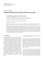
Table 1: Results with ground truth.
Classes Multispectral Panchromatic Fusion Collaborative
Field 1 31.10% 24.98% 46.12% 99.83%
Field 2 75.92% 67.69% 99.23% 89.60%
Bridge 40.74% 79.17% 35.19% 58.80%
Building 42.24% 44.26% 67.92% 46.42%
Means 47.50% 54.02% 62.11% 73.66%
convenience, but any clustering method can be used in
the collaborative system. For each experiment ((a), (b),
(c), and (d)) each clustering method is assigned to one
image. Then, the collaborative system described in Section 3
is launched with the modifications added in Section 4 for
multiresolution handling, thanks to the georeferencing. The
K-Means algorithm is applied on each image (step 1) with
different number of clusters (randomly piked in [8; 10]),
and initialized randomly (different initialization for each
method). Then, the clustering methods collaborate through
the refinement step and modify their results according to the
result of the other methods (step 2). Finally, the different
results obtained are combined in a single one, thanks to
a voting algorithm (step 3). Figure 10 presents the final
unification result (obtained from the vote of the different
methods) for the four test cases.
All the final results have seven clusters, due to the
capacity of the collaborative method to find a consensual
number of clusters. According to the interpretation of the
geographer expert, the following conclusions can be made.
The panchromatic case (Figure 10(b))hasproducedaquite
bad result where a part of the vegetation has been merged
with the water because of the lack of spectral information
to describe the pixels (i.e., only one band). The fusion case
(Figure 10(c)) has produced a result with a good spatial
resolution, but has failed to find some real classes (i.e., the
expert expected two clusters of vegetation which have been
merged). The multispectral case (Figure 10(a))hasproduced
a quite good result, but with a low spatial resolution. Finally,
the multisource collaboration (Figure 10(d))hasproduceda
good result with a good spatial resolution, and has corrected
some mistakes which appear on the multispectral case. For
(a) Multispectral (7 clusters) (b) Panchromatic (7 clusters)
(c) Fusion (7 clusters) (d) Multisource collaboration (7
clusters)
Figure 10: Results for the four test cases studied.
example, the field on the top-right of the area has been
identified more precisely thanks to the collaboration with the
panchromatic image (Figure 11).
To validate these interpretations, a ground truth has
been provided by the expert as partial binaries masks
(Figure 11(b)) for four classes. For each ground truth classes,
the most potential cluster was selected by the expert (the best
overlapping cluster as defined by the Vinet index in [24]). An
accuracy index has been computed as the ratio of the number
of pixels in the ground truth classes, and the number of pixels
of the cluster overlapping it. The results are presented in
Germain Forestier et al. 9
(a) Raw image (b) Ground truth
(c) Multispectral (d) Panchromatic
(e) Fusion (f) Collaborative
Figure 11: Examples of fields detection. (b) illustrates the ground
truth for field (1) (on the left) and field (2) (on the right).
Ta ble 1. As expected, the collaborative solution has produced
the best results, especially for the fields detection.
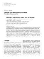
To study the evolution of the agreement amongst all the
clustering methods during the refinement step, the tools of
the theoretical framework of information theory [25]canbe
used. random variable. Then, the mutual information [26]
can be computed between a couple of clustering results.
The mutual information quantify the amount of information
shared by the two results. For two results R
i
and R
j
, the
[0; 1] normalized mutual information is defined as
nmi (R
i
, R
j
) =
2
p
n
i
k=1
n
j
l=1
log
n
i
·n
j
p.α
i,j
k,l
n
i
k
.n
j
l
, (13)
where p is the number of pixels to classify, n
i
is the number
of clusters from R
i
,andn
i
k
is the number of objects in the
cluster C
i
k
from R
i
.
Moreover, the average mutual information quantify the
shared information among an ensemble of clustering results,
and can be used as an indicator of agreement:
anmi (m)
=
1
N −1
N
j=1, j
/
=m
nmi (R
m
, R
j
) (14)
with m
= 1, 2, , N,andN the number of clustering results.
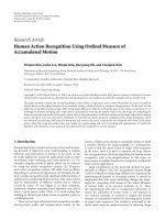
454035302520151050
Iteration
Anmi among the clustering methods
Anmi with the unified result
0.55
0.6
0.65
0.7
0.75
0.8
0.85
Anmi
Figure 12: Evolution of the anmi index among the clustering
methods and the average nmi between the results and the unified
result.
The average mutual information has been computed
during the refinement process which have produced the
result of Figure 10(d). Figure 12 presents the evolution of
the anmi index among the results of the different clustering
methods, and the average of the mutual information between
each clustering method and the unified result.
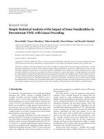
5.2. Multiresolution multidate collaboration
The second experiment was made on four images of a
coastal zone (Normandy Coast, Northwest of France). This
area is very interesting because it is periodically affected
by natural and anthropic phenomena which modify the
structure of the area. Consequently, the expert has often a
lot of heterogeneous images available which are acquired
through the years. Four images issued from three different
satellites (SPOT-4, SPOT-5 and ASTER) and having different
resolutions (20, 15, 10, and 2.5 meters) are used.
Four clustering methods were set up, each one using
one of the available images. As in the previous experiment,
the K-Means algorithm is ran on each image (step 1), the
refinement algorithm is then applied (step 2), and the results
are combined (step 3). Figure 14 presents the result of the
unification of the final results.
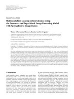
To make a better interpretation of the unified result,
a vote map is produced. This map represents the result of
the vote carried out during the combination of the results
[15]. Figure 15 presents the vote map corresponding to the
result shown in Figure 14. In this image, the darker the pixels
are, the less the clustering methods are in agreement. So,
the pixels where all the clustering methods agreed are in
white, and the black pixels represent a strong disagreement
amongst the clustering methods. This degree of agreement
is computed using the corresponding cluster (see (1)). This
representation helps the expert to improve his analysis of the
result, by concentrating his attention on the part of the image
where the clustering methods are in disagreement.
10 EURASIP Journal on Advances in Signal Processing
(a) SPOT-4-20 meters-3 bands (659 ×188)-date: 1999
(b) ASTER-15 meters-3 bands (922 ×256)-date: 2004
(c) SPOT-4-10 meters-3 bands (1382 ×384)-date: 2002
(d) SPOT-5-2.5 meters-3 bands (5528 ×1536)-date: 2005
Figure 13: The four images of Normandy Coast, France.
Figure 14: The final unification result.
Figure 15: The vote map.
Consequently, another way to improve the scene under-
standing and to show the agreement between the methods is
to visualise the corresponding clusters (1)betweenapairof
results. It allows the expert to see which parts of the clusters
are in agreement, and which parts are in disagreement, for
a couple of results. Figure 16 presents two corresponding
clusters between the clustering methods of this experiment.
(a) Corresponding clusters showing disagreement in the fields
(b) Corresponding clusters showing a part of the coast line
Figure 16: Corresponding clusters between two clustering meth-
ods, in grey the agreement, in black the disagreement.
In Figure 16(a), one can see the disagreement on a part of the
coast line. Figure 16(b) illustrates the disagreement on the
fields. All these results help the expert to improve his image
understanding.
6. CONCLUSIONS
In this paper, we have presented a method of multi-
source images analysis using collaborative clustering. This
collaborative method enables the user to exploit different
heterogeneous images in an overall system. Each clustering
method works on one image and collaborates with the other
clustering methods to refine its result.
Experimentations for the analysis of an urban area and a
coastal area have been presented. The system produces a final
result by combining the results of the different clustering
methods using a voting algorithm. The agreement and the
disagreement of the clustering methods can be highlighted
by a vote map, depicting the accordance between the different
clustering methods. Furthermore, the corresponding clusters
between a pair of clustering methods can be visualised.
These features are very useful to help the expert to better
understand his images.
However, there is still a lot of work for the expert
to really interpret the information in the dataset because
no semantic is given by the system. That is why we are
working on an extension of this process, integrating high-
level domain knowledge on the studied area (urban objects
ontology, spatial relationships, etc.). This should enable
to add automatically semantic to the result, giving more
information to the user.
ACKNOWLEDGMENTS
The authors would like to thank the members of the
FodoMuST and Ecosgil projects for providing the images and
the geographers of the LIV Laboratory for their help in the
interpretation of the results. This work is supported by the
french Centre National d’Etudes Spatiales (CNES Contract
70904/00).
Germain Forestier et al. 11
REFERENCES
[1] T. M. Mitchell, Machine Learning, McGraw-Hill, New York,
NY, USA, 1997.
[2] A. K. Jain, M. N. Murty, and P. J. Flynn, “Data clustering: a
review,” ACM Computing Surveys, vol. 31, no. 3, pp. 264–323,
1999.
[3] C. Pohl and J. L. Van Genderen, “Multisensor image fusion
in remote sensing: concepts, methods and applications,”
International Journal of Remote Sensing, vol. 19, no. 5, pp. 823–
854, 1998.
[4] Y. Chibani, “Selective synthetic aperture radar and panchro-
matic image fusion by using the
`
a trous wavelet decomposi-
tion,” EURASIP Journal on Applied Signal Processing, vol. 2005,
no. 14, pp. 2207–2214, 2005.
[5] Y L. Chang, L S. Liang, C C. Han, J P. Fang, W Y. Liang,
and K S. Chen, “Multisource data fusion for landslide clas-
sification using generalized positive boolean functions,” IEEE
Transactions on Geoscience and Remote Sensing, vol. 45, no. 6,
pp. 1697–1708, 2007.
[6] M P. Dubuisson and A. K. Jain, “Contour extraction of
moving objects in complex outdoor scenes,” International
Journal of Computer Vision, vol. 14, no. 1, pp. 83–105, 1995.
[7]M.Germain,M.Voorons,J M.Boucher,G.B.B
´
eni
´
e, and E.
Beaudry, “Multisource image fusion algorithm based on a new
evidential reasoning approach,” ISPRS Journal of Photogram-
metry & Remote Sensing, vol. 35, part 7, pp. 1263–1267, 2004.
[8] J. A. Benediktsson and I. Kanellopoulos, “Classification of
multisource and hyperspectral data based on decision fusion,”
IEEE Transactions on Geoscience and Remote Sensing, vol. 37,
no. 3, pp. 1367–1377, 1999.
[9] L. Bruzzone, R. Cossu, and G. Vernazza, “Combining paramet-
ric and non-parametric algorithms for a partially unsupervised
classification of multitemporal remote-sensing images,” Infor-
mation Fusion, vol. 3, no. 4, pp. 289–297, 2002.
[10] M. Fauvel, J. Chanussot, and J. A. Benediktsson, “Decision
fusion for the classification of urban remote sensing images,”
IEEE Transactions on Geoscience and Remote Sensing, vol. 44,
no. 10, part 1, pp. 2828–2838, 2006.
[11] A. Gionis, H. Mannila, and P. Tsaparas, “Clustering aggre-
gation,” in Proceedings of the 21st International Conference on
Data Engineering (ICDE ’05), pp. 341–352, Tokyo, Japan, April
2005.
[12] A. L. N. Fred and A. K. Jain, “Combining multiple clusterings
using evidence accumulation,” IEEE Transactions on Pattern
Analysis and Machine Intelligence, vol. 27, no. 6, pp. 835–850,
2005.
[13] A. Strehl and J. Ghosh, “Cluster ensembles—a knowledge
reuse framework for combining multiple partitions,” Journal
of Machine Learning Research, vol. 3, no. 3, pp. 583–617, 2003.
[14] Z H. Zhou and W. Tang, “Clusterer ensemble,” Knowledge-
Based Systems, vol. 19, no. 1, pp. 77–83, 2006.
[15] C. Wemmert and P. Ganc¸arski, “A multi-view voting method
to combine unsupervised classifications,” in Proceedings of the
2nd IASTED International Conference on Artificial Intelligence
and Applications (AIA ’02), pp. 362–324, Malaga, Spain,
September 2002.
[16] R. E. Bellman, Adaptive Control Processes, Princeton University
Press, Princeton, NJ, USA, 1961.
[17] G. F. Hughes, “On the mean accuracy of statistical pattern
recognizers,” IEEE Transactions on Informations Theory, vol. 14,
no. 1, pp. 55–63, 1968.
[18] L. I. Kuncheva, Combining Pattern Classifiers: Methods and
Algorithms, Wiley-Interscience, New York, NY, USA, 2004.
[19] W. Dou, Y. Chen, X. Li, and D. Z. Sui, “A general framework
for component substitution image fusion: an implementation
using the fast image fusion method,” Computers & Geosciences,
vol. 33, no. 2, pp. 219–228, 2007.
[20] V. Karathanassi, P. Kolokousis, and S. Ioannidou, “A com-
parison study on fusion methods using evaluation indicators,”
International Journal of Remote Sensing, vol. 28, no. 10, pp.
2309–2341, 2007.
[21] L. L. Hill, Georeferencing: The Geographic Associations of
Information, Digital Libraries and Electronic Publishing, The
MIT Press, Cambridge, Mass, USA, 2006.
[22] C. Li, L. Liu, J. Wang, C. Zhao, and R. Wang, “Comparison
of two methods of the fusion of remote sensing images
with fidelity of spectral information,” in Proceedings of the
IEEE International Geoscience and Remote Sensing Symposium
(IGARSS ’04), vol. 4, pp. 2561–2564, Anchorage, Alaska, USA,
September 2004.
[23] J. McQueen, “Some methods for classification and analysis of
multivariate observations,” in Proceedings of the 5th Ber keley
Symposium on Mathematical Statistics and Probability, vol. 1,
pp. 281–297, Berkeley, Calif, USA, June-July 1967.
[24] S. Chabrier, B. Emile, C. Rosenberger, and H. Laurent,
“Unsupervised performance evaluation of image segmenta-
tion,” EURASIP Journal on Applied Signal Processing, vol. 2006,
Article ID 96306, 12 pages, 2006.
[25] T. M. Cover and J. A. Thomas, Elements of Information Theory,
Wiley-Interscience, New York, NY, USA, 1991.
[26] A. Strehl, “Relationship-based clustering and cluster ensem-
bles for high-dimensional data mining,” Ph.D. thesis, The
University of Texas at Austin, Austin, Tex, USA, May 2002.