Báo cáo hóa học: "Research Article A Novel Semiblind Signal Extraction Approach for the Removal of Eye-Blink Artifact from EEGs" potx

Hindawi Publishing Corporation
EURASIP Journal on Advances in Signal Processing
Volume 2008, Article ID 857459, 12 pages
doi:10.1155/2008/857459
Research Article
A Novel Semiblind Signal Extraction Approach for
the Removal of Eye-Blink Artifact from EEGs
Kianoush Nazarpour,
1
Hamid R. Mohseni,
1
Christian W. Hesse,
2
Jonathon A. Chambers,
3
and Saeid Sanei
1
1
Centre of Digital Signal Processing, School of Engineering, Cardiff University, Cardiff CF24 3AA, UK
2
F. C. Donders Centre for Cognitive Neuroimaging, Kapittelweg 29, 6525 EN Nijmegen, The Netherlands
3
Advanced Signal Processing Group, Department of Electronic and Electrical Engineering, Loughborough University,
Loughborough, LE11 3TU, UK
Correspondence should be addressed to Kianoush Nazarpour,
Received 5 December 2007; Accepted 11 February 2008
Recommended by Tan Lee
A novel blind signal extraction (BSE) scheme for the removal of eye-blink artifact from electroencephalogram (EEG) signals is
proposed. In this method, in order to remove the artifact, the source extraction algorithm is provided with an estimation of the
column of the mixing matrix corresponding to the point source eye-blink artifact. The eye-blink source is first extracted and
then cleaned, artifact-removed EEGs are subsequently reconstructed by a deflation method. The a priori knowledge, namely, the

vector, corresponding to the spatial distribution of the eye-blink factor, is identified by fitting a space-time-frequency (STF) model
to the EEG measurements using the parallel factor (PARAFAC) analysis method. Hence, we call the BSE approach semiblind
signal extraction (SBSE). This approach introduces the possibility of incorporating PARAFAC within the blind source extraction
framework for single trial EEG processing applications and the respected formulations. Moreover, aiming at extracting the eye-
blink artifact, it exploits the spatial as well as temporal prior information during the extraction procedure. Experiments on
synthetic data and real EEG measurements confirm that the proposed algorithm effectively identifies and removes the eye-blink
artifact from raw EEG measurements.
Copyright © 2008 Kianoush Nazarpour et al. This is an open access article distributed under the Creative Commons Attribution
License, which permits unrestricted use, distribution, and reproduction in any medium, provided the original work is properly
cited.
1. INTRODUCTION
The electroencephalogram (EEG) signal is the superposition
of brain activities recorded as changes in electrical potentials
at multiple locations over the scalp. The electrooculogram
(EOG) signal is the major and most common artifact in EEG
analysis generated by eye movements and/or blinks [1]. Sup-
pressing eye-blink over a sustained recording course is par-
ticularly difficult due to its amplitude which is of the order
of ten times larger than average cortical signals. Due to the
magnitude of the blinking artifacts and the high resistance
of the skull and scalp tissues, EOG may contaminate the
majority of the electrode signals, even those recorded over
occipital areas. In recent years, it has become very desirable to
effectively remove the eye-blink artifacts without distorting
the underlying brain activity. In this regard, reliable and fast,
either iterative or batch, algorithms for eye-blink artifact
removal are of great interest for diverse applications such
as brain computer interfacing (BCI) and ambulatory EEG
settings. Various methods for eye-blink artifact removal from
EEGs have been documented that are mainly based on

independent component analysis (ICA) [1,Chapter2],linear
regression [2], and references therein. Approaches, such as
trial rejection, eye fixation, EOG subtraction, principal com-
ponent analysis (PCA) [3], blind source separation (BSS) [4–
6], and robust beamforming [7] have been also documented
as having varying success. A hybrid BSS-SVM method
for removing eye-blink artifacts along with a temporally
constrained BSS algorithm have been recently developed in
[5, 6]. Moreover, methods based on H
∞
[8] adaptive and
spatial filters [9] have also been presented in the literature for
eye-blink removal. It has been shown that the regression- and
BSS-based methods are most reliable [1, 2, 5–7, 10], despite
no quantitative comparison for any reference dataset being
available.
Statistically nonstationary EEG signals yield temporal
and spatial information about active areas within the brain
andhavebeeneffectively exploited for localizing the EEG
sourcesandtheremovalofvariousartifactsfromEEG
measurements. For instance, in [11] PCA is utilized to
2 EURASIP Journal on Advances in Signal Processing
decompose the signals into uncorrelated components where
the first component, the component with highest variance,
represents eye-blink artifact. However, the use of PCA
introduces nonuniqueness due to an arbitrary choice of
rotation axes. Although this nonuniqueness may be resolved
by introducing reasonable constraints, recently, ICA has
been applied to eliminate this problem by imposing the
statistical independence constraint which is stronger than the

orthogonality condition exploited by PCA [12]. However,
the eye-blink component should be identified manually
or in an automatic correction framework [5]ifoneuses
ICA. In these conventional methods, usually prior concepts
such as orthogonality, orthonormality, nonnegativity, and in
some cases even sparsity have been considered during the
separation process. However, such mathematical constraints
usually do not reflect specific physiological phenomena. In
essence, there are two different approaches for incorporating
prior information within the semiblind EEG source sepa-
ration (extraction); firstly, the Bayesian method [13]which
introduces a probabilistic modeling framework by specifying
distributions of the model parameters with respect to prior
information. Often the probabilistic approach is too com-
plicated, analytically and practically, to be implementable
specifically in high-density EEG processing; slow conver-
gence drawback should also be highlighted. The second
more feasible approach proposes expansion of conventional
gradient-based minimization of particular cost functions by
including rational physiological constraints. Theoretically,
widely accepted temporally or spatially constrained BSS
(CBSS) [5, 14–16] algorithms are the outcome of above-
mentioned methodology. However, CBSS methods still suffer
from extensive computational requirements (unlike blind
source extraction methods, i.e., [17]) of source separation
and severe uncertainties regarding the accuracy of the priors.
Simple and straightforward priors, such as the spectral
knowledge of ongoing EEGs or spatial topographies of some
source sensor projections, can be realistically meaningful in
semiblind EEG processing. In this regard, an interesting work

on topographic-time-frequency decomposition is proposed
in [18] in which, however, two mathematical conditions
on time-frequency signatures, namely, minimum norm and
maximal smoothness, are imposed. It has been shown
that these conditions may provide a unique model for
EEG measurements. Consolidating [18], recently in [19]
the space-time-frequency (STF) model of a multichannel
EEG has been introduced by using parallel factor analysis
(PARAFAC) [20]. More recently, we have utilized the STF
model for the first time in single trial EEG processing
for brain computer interfacing, where spatial signature of
selected component is employed as a feature vector for
classification purpose [1, 21].
In this paper, a novel physiologically inspired semiblind
signal extraction technique for removing the eye-blink
artifacts from single trial multichannel EEGs is presented.
Our SBSE method is based on that introduced in [17], while
by investigating the STF signatures of extracted factor(s)
by PARAFAC, the eye-blink factor is automatically selected
and its spatial distribution is exploited in the separation
procedure as a prior knowledge. The main advantages of our
method are as follows:
(1) in the BSS- and CBSS-based methods [4, 6, 15, 16, 22–
24], identification of the correct number of sources is
an important issue and requires high computational
costs. However, the simplicity of our method is due
to using the spatial a prior information to guarantee
that the first extracted source is the one of interest,
that is, the eye-blink source. Therefore, there is no
need to extract other sources which significantly

reduces the computational requirements. EEGs are
then reconstructed in a batch deflation procedure;
(2) unlike methods presented in [4, 5], there is no need to
compute objective criteria for distinguishing between
eye-blink and spurious peaks in the ongoing EEGs;
(3) unlike the regression-based methods [25], the pro-
posed method does not need any reference EOG
channel recordings (typically three channels);
(4) there is no need to separate the dataset into training
andtestingsubsetsasin[6]. As long as, by using
any primitive method we identify an eye-blink event,
the presented method can be utilized to remove the
artifact from EEGs.
This paper is organized as follows. In Section 2,we
present the SBSE method and compare its performance
to that of an existing spatially constrained BSS algorithm
presented in [16]. Afterwards, we briefly review the funda-
mentals of the PARAFAC method in Section 2.2 and suggest
our effective procedure to identify the spatial signature of
the eye-blink relevant factor. The results are subsequently
reported in Section 3, followed by concluding remarks in
Section 4
.
2. ALGORITHM DEVELOPMENT
Eye-blink contaminated EEG measurements at time t are
assumed as N zero-mean real mutually uncorrelated sources
s(t)
= [s
1
(t),s

2
(t), , s
N
(t)]
T
, where [·]
T
denotes the vector
transpose, mixed by an N
× N real full column rank matrix
A
= [a
1
, a
2
, , a
N
], where generally a
i
is the ith column of
A and specifically a
j
is the column of A corresponding to
the eye-blink source s
j
. The vector of time mixture samples
x(t)
= [x
1
(t), x

2
(t), , x
N
(t)]
T
is given as
x(t)
= As(t)+n(t), (1)
where n(t)
= [n
1
(t), n
2
(t), , n
N
(t)]
T
is the additive white
Gaussian zero-mean noise. We assume that the noise is
spatially uncorrelated with the sensor data and temporally
uncorrelated. Since the sources are presumed to be uncor-
related, the time lagged autocorrelation matrix R
k
can be
calculated as
R
k
= E

x(t)x

T

t −τ
k

=
N

i=1
r
i

τ
k

a
i
a
T
i
(2)
for k
= 1, 2, ,K,whereK is the index of the maximum
time lag, that is, τ
K
and E[·] denotes the statistical expecta-
tion operator. In (2), r
i
(τ
k

) = E[s
i
(t)s
i
(t − τ
k
)] is the time
lagged autocorrelation value of s
i
(t).
Kianoush Nazarpour et al. 3
2.1. Semiblind eye-blink signal extraction
The vector x(t)in(1), that is, recorded EEGs, is a linear
combination of the columns of the mixing matrix, that is,
the a
i
s, weighted by the associated source and contaminated
by sensor noise n(t). Therefore, the most straightforward
way to extract the jth source, the eye-blink artifact s
j
,
is to project x(t) onto the space in R
N
orthogonal to,
denoted by
⊥, all of the columns of A except a
j
, that is,
{a
1

, , a
j−1
, a
j+1
, , a
N
}. Hence, by defining a vector p ⊥
{
a
1
, , a
j−1
, a
j+1
, , a
N
} and q ≡ a
j
, and adopting the
notation of an oblique projector [17, 26], we may write
y(t)q
= E
q|p
⊥
x(t), (3)
where y(t) is an estimate of one source, say s(t), and
p
⊥
denotes the space in R
N

orthogonal to p, that is,
{a
1
, , a
j−1
, a
j+1
, , a
N
}.In(3), E
q|p
⊥
= qp
T
/p
T
q repre-
sents the oblique projection of q onto the space p
⊥
.Then,
y(t) can be extracted using the spatial filter p as
y(t)
= p
T
x(t)(4)
in which the scalar 1/p
T
q has been omitted and q has been
dropped from both sides of (3). In second-order statistics-
based BSE [17], both p and q are unknown and in order

to extract one source the following cost function has been
proposed:


d, p, q

= arg min
d,p,q
J
M
(d, p, q), (5)
where J
M
(d, p, q) =

K
k=1
R
k
p −d
k
q
2
2
, d is a column vector
d
= [d
1
, d
2

, , d
K
]
T
and ·
2
2
denotes the squared Euclidean
norm. We employ multiple time lags instead of a single time
lag which minimizes the chance, in practice, of the time-
lagged autocorrelation matrices employed having duplicate
eigenvalues and, hence, leading to failure in the extraction
process [5]. The cost function J
M
utilized in (5) exploits
the fact that for BSE, R
k
p should be collinear [27]withq
incorporating the coefficients d
k
which provides q with the
proper scaling. The trivial answer for (5)isd
= p = q = 0.
This solution has been avoided by imposing the condition
q
2
=d
2
= 1. Successful minimization of (5)leadsto
the identification of p, which extracts the source of interest

(SoI) in (4).
The main advantage of using (5)forBSEoverother
conventional BSE methods which incorporate higher order
statistics [12] is that it is indeed computationally simple and
efficient for extraction of nonstationary sources. However,
fundamentally in BSE, in the course of extraction, it is not
possible to tune the algorithm to extract the SoI as the
first extracted source in order to significantly decrease the
processing time which is essential in real-time applications.
Therefore, some prior knowledge should be incorporated
into the separation process to extract only the SoI. To this
end, we consider an auxiliary cost function
J
Aux
=
K

k=1


b
k
q −q
est


2
2
,(6)
where b is a column vector b

= [b
1
, b
2
, , b
K
]
T
and q
est
is
prior spatial information of the eye-blink source, that is, the
estimation of q, provided by PARAFAC (Section 2.2).
By minimizing J
Aux
coupled with (5) in a Lagrangian
framework, that is, J
tot
= J
M
+η
q
J
Aux
,weeffectively extract the
SoI as the first extracted source. Moreover, as it will be shown
in Section 3, including J
Aux
has significant incremental effect
in the minimization and results in faster convergence of J

tot
.
In mathematical terms the novel cost function is


b,

d, p, q

=
arg min
b,d,p,q
K

k=1



R
k
p −d
k
q


2
2
+ η
q



b
k
q −q
est


2
2

,
(7)
where η
q
is the Lagrange multiplier. In (7), the b
k
, k =
1, 2, , K values are free parameters to scale q during an
iterative solution to (7)and
b
2
= 1.
Essentially, there are two approaches in using the spatial
priors which vary the degree of freedom of the optimizing
process, that is, (7). In the optimizing procedures, we can
either strictly minimize the difference between q and q
est
iter-
atively as much as possible regardless of the probable errors
while estimating q

est
or on the other hand, by employing a
milder approach and allowing q in the optimization process
to deviate from the prior vector q
est
by an l
2
-norm-bounded
threshold. In mathematical terms, in soft constraining, we
consider δ
= q −q
est
as the estimation error where δ
2
< ;
 is a known positive constant. For the majority of spatially
constrained BSS applications, that is, [16, 22] and references
therein, the latter conservative approach is preferable to
strict ones, even if q
est
is accurately estimated. However,
to the authors’ belief, for eye-blink artifact removal from
EEGs hard constraining the extraction algorithm is sufficient
since sparsely occurring eye-blink is the dominant source
superimposed on EEGs. Therefore, the estimation of q
est
is trustworthy. We, in this paper, have explored the former
approach and assumed that the estimation of q
est
by the

PARAFAC-based STF model is accurate enough. We have
also experimentally found that although the introduction of
b in (7) does not have any rotational effect on q,itdoes
result in better minimization of J
tot
. The interested reader
is referred to [7] in which we have realized a conservative
method for the eye-blink artifact removal from the EEGs.
The solution to (7) is found by alternatively adjusting
its parameters, that is, an alternating least squares (ALS)
method. We iteratively update each of the four unknown
vectorstillconvergence.Firstly,wefixq, d,andb and update
p. Taking the gradient of J
tot
with respect to p leads to an
optimal analytical solution for p as
∂J
tot
∂p
= 2
K

k=1
R
k

R
k
p −d
k

q

=
0,
p
⇐= Q

K

k=1
d
k
R
k

q; Q =

K

k=1

R
k

2

−1
,
(8)
where a

⇐ b denotes replacing a by b.Thereafter,wefixp,
b,andq and update d.Asin[17], utilizing the property that
4 EURASIP Journal on Advances in Signal Processing
q
2
= 1, the gradient of J
tot
with respect to d
k
becomes
∂J
tot
∂d
k
=−2
K

k=1


R
k
p

T
−d
k
q
T


q = 0, k = 1, 2, , K.
(9)
The update rule for d is as
d
⇐=
u
u
2
; u =

r
T
1
q, r
T
2
q, , r
T
k
q

T
, (10)
where r
k
= R
k
p. Then, fixing p, d,andb,weadjustq while
ensuring
q

2
= 1. Consider
∂J
tot
∂q
=−2
K

k=1
d
k
r
k
−2η
q
K

k=1
b
k
q
est
+2(1+η)q = 0 (11)
and q is adjustable by
q
⇐=
v
v
2
; v =

K

k=1

d
k
r
k
+
1
K
η
q
b
k
q
est

. (12)
For updating b, the rest of the variables are fixed, that is,
q, p,andd and we proceed by minimizing (7)withrespectto
b
k
, that is,
∂J
tot
∂b
k
= 2η
q

K

k=1

b
k
−q
T
est
q

=
0. (13)
b is updated as
b
⇐=
w
w
2
; w =

q
T
est
q, q
T
est
q, , q
T
est

q

. (14)
We re ta in b as a vector instead of a scalar to present a
consistent formulation. Finally, in order to solve (7) for the
Lagrange multiplier, that is, η
q
,wedefinevectore
i
as a vector
whoseelementsareallzeroexceptfortheith component
which is one, that is, e
i
= [0, ,0,1,0, ,0]
T
, ∀i ∈{1, 2,
, K
}. Considering that v =

K
k=1
(d
k
r
k
+(1/K)η
q
b
k
q

est
)in
(12), η
q
can be easily updated by putting v = 0aftereach
iteration. Therefore, we assign a new value for η
q
as
η
q
=

1/b
i

v −

K
k=1
d
k
r
k

T
e
i
q
T
est

e
i
. (15)
The performance of the proposed semiblind signal
extraction procedure has been evaluated through a compar-
ison with the spatially constrained blind signal separation
(SCBSS) algorithm proposed in [16, 22] for a set of synthetic
mixtures of analytic sources.
Four signal sources, namely, two sinusoids of frequencies
of 10 Hz and 12 Hz representing brain rhythmic waves, a
spiky source standing for eye-blink artifact and a white Gaus-
sian distributed signal as the background brain activity have
been synthetically mixed. The mixing matrix A (generated
randomly from a standardized normal distribution) used in
this paper is
A
=
⎡
⎢
⎢
⎢
⎢
⎢
⎢
⎣
0.5594 0.5923 0.2101 0.1685
0.4676
−0.2133 0.3478 −0.7046
0.0916 0.3763 0.9058
−0.6718

0.6783
−0.6797 0.1201 −0.1545
⎤
⎥
⎥
⎥
⎥
⎥
⎥
⎦
. (16)
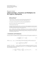
The source waveforms and the mixtures are presented in
Figures 1(a) and 1(b). The source signals have been selected
as such in order to cover the range of sub-Gaussianity to
super-Gaussianity. The original mixtures have been plotted
in Figure 1(b) in solid blue lines, where x
2
and x
3
are highly
affected by the spiky source, s
4
. Here, the objective is to
visually compare our proposed method with that of [16]
in which a spatially constrained blind source separation
(SCBSS) method based on FastICA [12]hasbeensuggested
for eye-blink artifact removal. In Figure 1(b), the outcome
of our semiblind signal extraction method has been plotted
in red solid lines which has effectively removed the s
4

signal from the mixtures. It is also worth considering
the clean artifact free parts of the mixtures which have
been reconstructed perfectly. Moreover, the outputs of the
established method of [16] in artifact removal from EEGs
have been shown in solid green lines. Evidently, the outcome
of our method does overlap that of [16]. The correlation
coefficient (CC) of two discrete random variables x and y
over a fixed interval is mathematically defined as:
CC
=



w
i=1
x(i)y(i)




w
j
=1
x
2
(j)


w
j

=1
y
2
(j)
, (17)
where w is the number of time samples. Figure 1(c),demon-
strates averaged CC values between segments of cleaned
mixtures (after removing s
4
) and original mixtures by using
proposed method and that of [16, 22]. CC values of about
unity show that SBSE method provide similar results as to
SCBSS.
In these simulations, we have presumed that spatial
distribution (signature) of the source of interest, s
4
,is
known in advance. This assumption helps to validate our
SBSE method comparing to [16, 22]regardlessofhow
accurate various existing methods perform in estimating the
aforementioned vector.
Moreover, through simulation studies we have found
consistent faster convergence of our optimization scheme,
as reported in Section 3,ascomparedtothatin[17]which
highlights that incorporating auxiliary cost function J
Aux
into
extraction process significantly upgrades the performance.
Next, we establish how PARAFAC is utilized to provide the
required a prior information.

2.2. PARAFAC
PARAFAC is a widely accepted tool in extracting disjoint
multidimensional phenomena with application to food sci-
ence, communications, and biomedicine [7, 10, 19–21, 28–
31]. In this paper, by exploiting PARAFAC, we decompose
the eye-blink contaminated EEG measurements in order to
extract the factor relevant to the eye-blink artifact for use
within the SBSE. The resulting spatial signature of the eye-
blink-related factor, that is, q
est
is exploited to formulate (7).
The spatial signatures of this factor is directly related to the
level of eye-blink contamination for each electrode and is
thereby comparable to the column of the mixing matrix that
propagates the point source eye-blink artifact into the EEG
channels. Physiologically, this assumption is rational since
Kianoush Nazarpour et al. 5
−10
0
15
s
4
−10
0
10
s
3
−10
0
10

s
2
−10
0
10
s
1
Source signals
0123
Time (s)
(a)
−4
0
4
x
4
−4
0
4
x
3
−4
0
4
x
2
−4
0
4
x

1
Mixtures
0123
Time (s)
0123
0123
0123
(b)
0.7
0.8
0.9
1
Correlation coefficients
x
1
x
2
x
3
x
4
CC
SCBSS [16]
Proposed SBSE, K
= 25
(c)
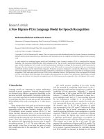
Figure 1: Simplified scalp EEG measurements; brain source signals in (a) and mixed recordings (b). (a) shows four synthetic sources,
namely, s
1
and s

2
which represent brain rhythmic activities, s
3
for background white noise, and s
4
the eye-blink artifact source. (b) illustrates
the mixed signals in solid blue lines, that is, x,wherex
2
and x
3
are highly contaminated by the eye-blink source, s
4
. The artifact removed
mixtures have been also plotted by using our proposed method, plotted in solid red, and that of [16] in solid green lines. Evidently, our
proposed method presents reasonably similar performance to that of the semiblind separation method in [16]. In (c), the averaged CC
values between the segments of cleaned mixtures (after removing s
4
) and the original mixtures by using SBSE method and SCBSS algorithm
in [16] have been depicted. CC values of about unity again justify that the SBSE method provides similar results as to SCBSS.
eye-blink is attenuated while propagating from frontal to
central and occipital areas of the brain.
In our approach, the multichannel EEG data are trans-
formed into time-frequency domain. This gives the two-way
EEG recording, that is, the matrix of space(channel)-time,
an extra dimension and yields a three-way array of space-
time frequency. In other words, for I EEG channels, we
compute the energy of the time-frequency transform for J
time instants and K frequency bins. By stacking these I
matrices (of size J
× K) and adopting the Matlab matrix

notation, we set up the three-way array X
I×J×K
≡ X(1 :
I,1:J,1:K) and introduce it to PARAFAC.
Conventional methods, for instance, PCA or ICA, ana-
lyze such data by unfolding some dimensions into others,
reducing the multiway array into matrices. However, the
aforementioned unfolding procedures make the interpreta-
tion of the results ambiguous since they remove specific
information endorsed by those dimensions. Consequently,
rather than unfolding these multiway arrays into matrices,
we exploit PARAFAC to explore the space-time-frequency
(STF) model of EEG recordings. The key idea behind this
research is in considering EEGs as superposition of neural
electro-potentials. EEGs may be represented by using the
linear models which are defined in three domains, that
is, space, time, and frequency, in order to simultaneously
investigate their spatial, temporal, and spectral dynamics
[1, 7, 10, 19, 21, 30]. Here, we have assumed that each distinct
local EEG activity (on the scalp) is uncorrelated with the
activities of the neighboring areas of the brain. EEGs can
be modeled as sum of the distinct components where each
distinct component is formulated as the product of its basis
in space, time, and frequency domains. The interested reader
is referred to [28, 29, 32] for further mathematical details
of the PARAFAC model, the uniqueness conditions, and its
robust iterative fitting which are out of the scope of this
paper.
6 EURASIP Journal on Advances in Signal Processing
Complex wavelet transform

To setup a three-way array, in the present study, a continuous
wavelet transform is utilized to provide a time-varying
representation of the energy of the signals over all channels.
The complex Morlet wavelets w(t, f
0
), with σ
f
= 1/(2πσ
t
),
and A
= (σ
t
√
π)
−1/2
, are used here in which the tradeoff
ratio ( f
0
/σ
f
) is 7, to create a wavelet family. This wavelet
configuration is known to be optimized in EEG processing
[19]. The time-varying energy E(t, f
0
)ofasignalataspecific
frequency band is the squared norm of the convolution of
a complex wavelet of the signal x(t), that is, E(t, f
0
) =

|
w(t, f
0
)∗x(t)|
2
,where∗stands for the convolution product
andthemodulusoperatorisdenotedby
|·|.
In mathematical terms, the factor analysis is expressed as
X
I×J
= U
I×F
(S
J×F
)
T
+ E
I×J
where U is the factor loading,
S the factor score, E the error, and F the number of factors.
Similarly, the PARAFAC for the three-way array X
I×J×K
is
presented by unfolding one modality to another as
X
I×JK
= U
I×F


S
K×F
D
J×F

T
+ E
I×JK
, (18)
where D is the factor score corresponding to the second
modality and S
 D = [s
1
⊗ d
1
, s
2
⊗ d
2
, , s
F
⊗ d
F
] is the
Khatri-Rao product and
⊗ denotes the Kronecker product
[33]. Equivalently, the jth matrix corresponding to the jth
slice of the second modality of the 3-way array is expressed
as
X

I×j×K
= U
I×F
D
F×F
j

S
K×F

T
+ E
I×j×K
, (19)
where D
j
is a diagonal matrix having the jth row of D along
the diagonal. ALS is the most common way to estimate the
PARAFAC model. In order to decompose the multiway array
to parallel factors the cost function (normally the squared
error) is minimized as in [20]


U,

S,

D

=

arg min
U,S,D



X
I×JK
−U
I×F

S
K×F
D
J×F

T



2
2
.
(20)
Here, X
I×J×K
is the three-way array of wavelet energy of
multichannel EEG recordings and U
I×F
, S
K×F

,andD
J×F
denote the spatial, temporal, and spectral signatures of
X
I×J×K
, respectively. In this paper, the trilinear alternating
least squares (TALSs) method [34]isusedtocompute
the parameters of the STF model. We in [7], inspired by
[30], have proposed a novel computationally simple method
for STF modeling of EEG signals in which in order to
reduce the complexity present in the estimation of the STF
model using the three-way PARAFAC, the time domain
is subdivided into a number of segments and a four-way
array is then set to estimate the space-time-frequency-
time/segment (STF-TS) model of the data using the four-
way PARAFAC. Subsequently, the STF-TS model is shown to
approximate closely the classic STF model, with significantly
lower computational cost.
In summary, our method consists of the following stages.
Given an artifact contaminated EEG data, we
(1) bandpass filter the EEGs between 1 Hz and 40 Hz,
(2) set up the three-way array, that is, X
I×J×K
, as stated in
Section 2.2,
(3) execute PARAFAC and select the eye-blink artifact
relevant factors as will be fully described in Section 3,
(4) exploit the spatial signature of the eye-blink artifact
factor in SBSE cost function (7),
(5) reconstruct the artifact removed EEGs in a deflation

framework. See the appendix.
3. RESULTS
We applied the SBSE algorithm to real EEG measurements.
The database was provided by the School of Psychology,
Cardiff University, UK, and contains a wide range of eye-
blinks and, therefore, gives a proper evaluation of our
method. The scalp EEG was obtained using 28 Silver/Silver-
Chloride electrodes placed at locations defined by the 10–
20 system [1]. EEGs have been recorded to provide a
reference dataset specifically for the purpose of evaluating
different artifact removal methods from one healthy subject
and contains numerous eye-blinks, eye movements, and
motion artifacts. The data were sampled at 200 Hz, and
bandpass filtered with cut-off frequencies of 1 Hz and
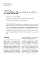
40 Hz. In order to reduce the computational costs of the
PARAFAC modeling, we selected 16 channels out of the
above-mentioned 28 channels as illustrated in Figure 2.
Each EEG segment was transformed into the time-
frequency domain by means of the complex wavelet trans-
form where the frequency band from 2 Hz to 25 Hz with
resolution of 0.1 Hz has been considered. This three-way
array is then introduced to PARAFAC where the number
of factors is selected as one or two, as highlighted in the
following experiments, identified by using the method of
core consistency diagnostic (CORCONDIA) [35]. Automat-
ically, PARAFAC identifies the most significant factors with
CORCONDIA values greater than a set threshold, that is,
85% [35], within each recording. Two sample results are
demonstrated here in order to elaborate the potential of our
method.

3.1. Experiment 1
Figure 2(a) shows EEG measurements which are contam-
inated with two eye-blinks at approximate times of two
and half and five seconds. The effects of the eye-blinks are
evident mostly in the frontal electrodes, namely, FP1, FP2,
F3, F4, F7, and F8. However, central C3 and C4 and occipital
O1 electrodes are also partly affected. Implementation of
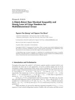
PARAFAC on this measurement results in the STF model,
the spectral, temporal, and spatial signatures which are
depicted in Figures 3(a) to 3(c). Although there are two eye-
blinks, CORCONDIA suggests the number of factors F to
be one as in Figure 3(d). This value is rational since both
of the eye-blinks originate from a certain vicinity (frontal
lobe of the brain) and occupy the same frequency band
and there is no significant brain background activity. By
using spatial distribution of the extracted factor as a prior
information, eye-blink artifacts are effectively removed. In
Kianoush Nazarpour et al. 7
FP1
FP2
F3
F4
C3
C4
P3
P4
O1
O2
F7
F8

T3
T4
T5
T6
Before artifact removal
0246
Time (s)
(a)
FP1
FP2
F3
F4
C3
C4
P3
P4
O1
O2
F7
F8
T3
T4
T5
T6
After artifact removal
0246
Time (s)
(b)
Figure 2: The result of the proposed eye-blink artifact removal
method for a sample of real EEG signals recorded from the selected

16 electrodes. In (a), the EOG is evident just after the time 2 seconds
and more prominent on the frontal electrodes, that is, FP1 and FP2.
However, in (b), the same segment of EEG after being corrected for
eye-blink artifact using the proposed algorithm is illustrated. Note
the small spike-type signals, indicated by arrows, right after the first
eye-blink are precisely retained after eye-blink artifact removal.
order to minimize (7) initial values of the vectors b, d,
p,andq independently drawn from standardized normal
distributions N(0, 1), η
q
is initialized to 5 and q
est
is set to the
spatial signature of the extracted factor. Figure 4 compares
the average value of 10log
10
(J
tot
/NK ) over 50 independent
runs. Two scenarios have been devised by varying the
number of time lags, that is, K
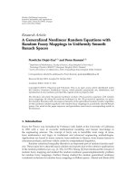
= 10 and 25. Note that in
[17], J
tot
= J
M
.Evidently,inbothscenarios,performanceof
proposed SBSE method is superior to that of the method
in [17]. After approximately 10 iterations, the extracting
vector p is identified. Furthermore, by incorporating the

prior knowledge, it is guaranteed that p extracts the eye-
blink source. The effect of the eye-blink is then removed from
the multichannel EEG using the batch deflation algorithm in
[36]. The impressive issue on the resolution of the proposed
algorithm is that it does not affect the very low amplitude
spike-type signals right after first eye-blink, indicated by
arrows, during extraction process, Figure 2.
3.2. Experiment 2
Performance of the method with same initial values for
another set of EEGs from the database is demonstrated
in Figure 5 where in left subplot, the truncated 4 seconds
of EEG recordings before and after eye-blink removal
processing are plotted. Figure 5(b) illustrates averaged corre-
lation coefficients between artifact removed channel signals
and original contaminated ones with their corresponding
standard deviations over 25 independent runs. As expected,
CC values corresponding to the signals recorded from
0
1
2
3
4
5
6
×10
3
Loading
Spectral signature of
the extracted factor
2 5 10 15 20 25

Frequency (Hz)
(a)
0
0.01
0.02
0.03
0.04
0.05
0.06
0.07
Loading
Temporal signature of
the extracted factor
123456
Time (s)
(b)
Spatial signature of
the extracted factor
(c)
0
20
40
60
80
100
CORCONDIA
123
Factor
(d)
Figure 3: The extracted factor by using PARAFAC; (a) and (b)

illustrate, respectively, the spectral and temporal signatures of the
extracted factors and (c) represents the spatial distribution of the
extracted factor which has been considered as the a prior knowledge
during extraction procedure, (d) shows that the number of factors F
suggested by CORCONDIA to be one since the bars corresponding
to F
= 2andF = 3 are less than the threshold, that is, 85%.
frontal electrodes are relatively low showing these signals are
significantly altered; artifact removed. However, values cor-
responding to other channel signals, that is, parietal, central,
temporal, and occipital, are almost unity demonstrating that
our algorithm does not affect clean EEG measurements.
The STF model of this recording is introduced by
PARAFAC. In contrast to previous experiments, CORCON-
DIA suggests F
= 2 since PARAFAC identified a significant
brain background activity during occurrence of eye-blink.
Figures 6(a) to 6(d) illustrate the estimated signatures of
16-channel EEG signal contaminated by eye-blink. The
first component (factor 1) of the STF model demonstrates
the eye-blink-relevant factor. (1) It mainly occurs in the
frequency band of around 5 Hz while the other factor exists
in the entire band and represents the ongoing activity of the
brain or perhaps a broadband white noise-like component,
Figure 6(a). (2) The temporal signature of the first factor
definitely shows a transient phenomenon such as eye-blink
while that of Factor 2 consistently exists in the course of
EEG segment, Figure 6(b).(3)UnlikeinFigure 6(d),in
Figure 6(c), the spatial distribution of the extracted factor is
confined to the frontal area, which clearly demonstrates the

effect of eye-blink. The other factor shows the background
activity of the brain as it spreads all over the scalp.
Hence, we employ spatial distribution of the first
extracted factor in the SBSE.
8 EURASIP Journal on Advances in Signal Processing
−60
−50
−40
−30
−20
−10
10 log
10
(J
tot
/(NK))
0 50 100 150
Number of iterations
BSE [17], K
= 10
Proposed SBSE, K
= 10
(a)
−70
−60
−50
−40
−30
−20
10 log

10
(J
tot
/(NK))
0 50 100 150
Number of iterations
BSE [17], K
= 25
Proposed SBSE, K
= 25
(b)
Figure 4: The averaged (over 50 independent runs) convergence characteristics, 10 log
10
(J
tot
/NK), of the SBSE and BSE of [17] are depicted
for two values of K, that is, 10 in (a) and 25 in (b). In both subplots the solid and dashed curves correspond, respectively, to the proposed
SBSE and BSE of [17].
FP1
FP2
F3
F4
C3
C4
P3
P4
O1
O2
F7
F8

T3
T4
T5
T6
Before and after artifact correction
01234
Time (s)
(a)
0
0.2
0.4
0.6
0.8
1
FP1
FP2
F3
F4
C3
C4
P3
P4
O1
O2
F7
F8
T3
T4
T5
T6

Averaged CC
Channels
Resolution in reconstruction
(b)
Figure 5: The results of the proposed eye-blink artifact removal method for a set of real EEG signals recorded from 16 electrodes; (a) shows
the eye-blink contaminated EEGs in red and the artifact corrected EEGs in blue where the eye-blink artifact is evident just before time
2 seconds and more prominent on the frontal electrodes, that is, FP1 and FP2. However, in (b), averaged CC values between the artifact
corrected channel signals and the original contaminated EEGs with their corresponding standard deviations over 25 independent runs are
plotted. CC values corresponding to the frontal channel signals are relatively lower than the values corresponding to other channel signals
which are almost unity, (b) illuminates how our algorithm reconstructs the artifact-freed EEGs faithfully without affecting clean signals
coming from nonfrontal areas.
3.3. Performance evaluations
In order to provide a quantitative measure of performance
for the proposed artifact removal method, the CC values of
the extracted eye-blink artifact source and the original and
the artifact removed EEGs are computed, see Figure 7.
ThevaluesreportedinFigure 7 have been computed
as follows. For each of the 20 different artifact contam-
inated EEGs, we executed our proposed algorithm. The
aforementioned CCsforeachrunwerethencomputed
between the extracted eye-blink and the EEGs before and
after the artifact removal. These values have subsequently
been averaged and shown in Figure 7. Furthermore, their
corresponding standard deviations have also been reported.
As expected, the CC values have been significantly decreased
by using the proposed method. Simulations for 20 EEG
measurements demonstrate that the proposed method can
efficiently identify and remove the eye-blink artifact from the
raw EEG measurements.
As a second criterion for measuring the performance of

the overall system, we selected a segment of EEG, called x
seg
and the reconstructed EEG x
seg
which does not contain any
artifact, and measured the waveform similarity by
η
dB
= 10 log

1
M
M

i=1

1 −E

x
seg
(i) − x
seg
(i)


. (21)
When the value of η
dB
is zero, the original and reconstructed
waveforms are identical. From the 20 sets of EEGs, the

Kianoush Nazarpour et al. 9
0
5
10
15
20
×10
2
Loadings
Spectral signatures
2 5 10 15 20 25
Frequency (Hz)
Factor 1
Factor 2
(a)
0
0.02
0.04
0.06
0.08
0.1
Loadings
01234
Time (s)
Temporal signatures
Factor 1
Factor 2
(b)
The spatial signature of factor 1
(c)

The spatial signature of factor 2
(d)
Figure 6: The extracted factors by using PARAFAC; (a) and (b)
illustrate, respectively, the spectral and temporal signatures of the
extracted factors; (c) and (d) present the spatial distribution of the
factors, respectively. Evidently, factor 1 demonstrates the eye-blink
phenomenon as it occurs in frequency band of around 5 Hz (a), it
is indeed transient in the time domain (b) and it is confined to the
frontal area.
0
0.2
0.4
0.6
0.8
1
Averaged CC
FP1
FP2
F3
F4
C3
C4
P3
P4
O1
O2
F7
F8
T3
T4

T5
T6
Before artifact removal
(a)
0
1
2
3
4
×10
−3
Averaged CC
FP1
FP2
F3
F4
C3
C4
P3
P4
O1
O2
F7
F8
T3
T4
T5
T6
After artifact removal
(b)

Figure 7: The averaged CC values (and their corresponding
standard deviations) between the extracted eye-blink and the
restored EEGs before and after artifact removal of different channels
in (a) and (b), respectively. The experiments have been performed
for 20 different eye-blink contaminated EEG recordings. Note that
the scales are different by 10
3
.
average waveform similarity was as low as η
dB
= 0.01 dB
(standard deviation 10
−3
dB). These results suggest that the
observations have been faithfully reconstructed.
3.4. Robustness
As indicated earlier, in soft constrained blind source extrac-
tion (separation [16]) schemes, even if the estimation of
q
est
is slightly biased, the optimization algorithm takes that
into account and accommodates it during the extraction of
the source of interest. However, as indicated in Section 2.1,
in this paper a hard approach has been taken where
the algorithm strictly minimizes the cost function, in (7)
regardless of the probable errors or biases while estimating
q
est
.
Interestingly, the scenario is not actually as restricted as

it seems; that is, even if there is a small deviation in the
q
est
from the actual q which sounds quite rational, SBSE
is able to accommodate that without any need for further
formulations as in [16]. The truth lies in the alternating least
squares approach in updating q, that is, (12) where SBSE
tries to estimate the best set of q and p simultaneously both
ideally orthogonal to
{a
1
, , a
j−1
, a
j+1
, , a
N
} in order to
minimize the cost function (7). Therefore, even if q
est
+ δ
is utilized instead of the q
est
, as the result of STF modeling
and PARAFAC in the cost function (7), the optimization
process results in converging to the originally estimated q,
that is, q
est
. In the sequel the results of a series of experiments
with different δs are presented in order to consolidate the

proposed SBSE method for EB artifact removal. Let us
start with an experiment where instead of q
est
, q
est
+ δ
1
,is
introduced to SBSE where δ
1
is computed as
δ
1
= 0.1×r, (22)
where r is a vector of 16 elements ideally drawn from a zero-
mean and unit-variance normal distribution, that is, N (0,1).
Using (22), the norm of
δ
1

2
is highly likely to be less
than 0.6. Therefore, if
δ
1

2
< 0.6, it is probable that SBSE
compensates for the deviation of q
est

from q and extracts
the EB artifact. For instance in Figures 8 and 9, an example
has been provided where
δ
1

2
= 0.503. In Figure 8(a), q
est
obtained by PARAFAC is depicted which should be used in
(7). Figure 8(b) shows the perturbed q
est
by δ
1
which has
been replaced in (7) instead of q
est
and introduced to SBSE.
Finally, in Figure 8(c), the resulting q after the alternative
least squares optimization has been illustrated. Evidently,
Figure 8(c) is quite similar to Figure 8(a).
The result of the artifact removal is depicted in Figure 9.
EEG traces in red are the original artifact contaminated
recordings. Traces in blue are the resulting artifact removal
using the original estimate of q, that is, q
est
, by PARAFAC.
EEG plots in black, which entirely overlap with the blue
ones, are the resulting artifact restored EEGs by using the
artificially perturbed q

est
, that is, q
est
+ δ
1
put in (7).
Thereafter, instead of q
est
, q
est
+ δ
2
is introduced to SBSE.
The vector δ
2
is computed in the same way as δ
1
by keeping
the coefficient as 0.1 in (22), norm
δ
1

2
= 0.430. Since
q
est
+ δ
2
, Figure 10(b), is significantly different in steering
10 EURASIP Journal on Advances in Signal Processing

(a) (b) (c)
Figure 8: In (a), q
est
is depicted, (b) shows the deviated q
est
by δ
1
which has been put in (7) instead of q
est
, (c) illustrates the resulting
q after ALS optimization procedure.
FP1
FP2
F3
F4
C3
C4
P3
P4
O1
O2
F7
F8
T3
T4
T5
T6
Before and after artifact correction
01234
Time (s)

Figure 9: The result of the artifact removal from EEGs depicted in
Figure 5(a). EEG traces plotted in red color are the original artifact
contaminated signals. EEGs in blue color are the resulting artifact
removed signals using q
est
. Traces in black are the resulting artifact
restored EEGs by using q
est
+ δ
1
instead of q
est
.
direction from Figure 10(a), SBSE may not compensate for
the deviation δ
2
.InFigure 10(a), q
est
resulted by PARAFAC
is depicted which should have been put in (7). Figure 10(b)
shows the perturbed q
est
by δ
2
which has been replaced
in (7) instead of q
est
and introduced to SBSE. Finally, in
Figure 10(c), the resulting q after the alternative least squares
optimization has been illustrated. The vector plotted in

Figure 10(c) does not converge to the vector plotted in
Figure 10(a).
TheresultoftheartifactremovalisdepictedinFigure 11.
Again as Figure 9, the EEG traces in red are the original
artifact contaminated recordings. Traces in blue are the
resulting artifact removal using the original estimate on q,
that is, q
est
, by PARAFAC. However, EEG plots in black show
an absolute failure in artifact removal procedure by q
est
+ δ
2
.
It can be concluded that in order that the SBSE
presents a robust performance even if q
est
is perturbed by
a norm bounded small deviation, its direction should not
be changed. That is, if the bias is fairly distributed over the
elements of q
est
, since a normalized version q
est
is used in the
formulations, based on our experience, it is highly unlikely
that SBSE does not compensate for it.
(a) (b) (c)
Figure 10: In (a), q
est

is depicted, (b) shows the deviated q
est
by δ
2
which has been put in (7) instead of q
est
, (c) illustrates the resulting
q after ALS optimization procedure.
FP1
FP2
F3
F4
C3
C4
P3
P4
O1
O2
F7
F8
T3
T4
T5
T6
Before and after artifact correction
01234
Time (s)
Figure 11: The result of the artifact removal from EEGs depicted in
Figure 5(a). EEG traces plotted in red color are the original artifact
contaminated signals. EEGs in blue color are the resulting artifact

removed signals using q
est
. Traces in black are the resulting of the
unsuccessful artifact removal procedure by using q
est
+ δ
2
instead of
q
est
.
4. CONCLUDING REMARKS
It is generally accepted that the eye-blink artifact can be
removed from EEGs by using the BSS- and regression
based methods for multichannel EEGs data with/without
the reference EOG electrodes. However, nowadays this
challenging topic is tended to be solved by a semiblind
method rather than in a totally blind signal processing
framework [5, 7, 10, 15, 16, 22]. Notwithstanding these
recently published semiblind approaches, we propose an
analytic and rational method to acquire the prior informa-
tion, that is, the spatial signature of the eye-blink signal,
from the EEG measurements. Therefore, we do not follow
the conventional heuristic approaches such as that of [15]
where an approximation of the temporal structure of the
eye-blink source signal is included in ICA. Furthermore, to
the best of our knowledge, there has not been any method
specifically based on semiblind signal extraction for eye-
blink artifact removal from EEGs. The presented method is
computationally simpler than the spatially constrained blind

source separation method of [16, 22] since there is no need
to estimate all the columns of the mixing matrix A in (1).
Kianoush Nazarpour et al. 11
The vector of spatial distribution of the eye-blink factor
has been identified using PARAFAC. For the first time in this
work, we have utilized the vector of spatial signature of the
eye-blink factor resulted by the STF modeling of EEGs as
the estimation of the column vector of the mixing matrix
A that introduces the eye-blink source to the EEGs. This
assumption is rational since the eye-blink can be considered
as a strong point source which is merely attenuated while
propagating from frontal area to the central and occipital
parts of the brain. This spatial distribution of the eye-blink
factor then has been incorporated to our SBSE algorithm.
The EEGs are processed using the time-lagged second-order
SBSE algorithm and the artifact is autonomously extracted;
then, the EEGs are reconstructed in a deflation framework.
Based on our experiments, the proposed SBSE algorithm
consistently removes the eye-blink artifacts from the EEG
signals.
APPENDIX
THE DEFLATION METHOD
In order to achieve EB-free EEG recordings, x
filt
(t), after
the extraction of the EB source y(t) using (4), we apply
the deflation procedure which eliminates the previously
extracted signal, y(t), from the recording mixtures, that is,
x(t):
x

filt
(t) = x(t) − py(t), (A.1)
where, as in [36, Section 5.2.5],
p can be estimated either
adaptively or simply after minimization of the mean square
cost function J with respect to
p:
J(
p) = E

x
filt
(t)
T
x
filt
(t)

=
E

x(t)
T
x(t)

−
2p
T
E


x(t)y(t)

+ p
T
pE

y
2
(t)

.
(A.2)
This results in the following efficient batch one-step formula
to estimate
p:
p =
E

x(t)y
T
(t)

E

y(t)
2

=
E


x(t)x
T
(t)

p
E

y(t)
2

,(A.3)
where p is achieved by (8). In fact,
p is an estimation of
a
j
, the jth column of A, neglecting arbitrary scaling and
permutations of columns ambiguities.
ACKNOWLEDGMENTS
This work is supported in part by The Leverhulme Trust,
UK, and Cardiff University, UK. The authors would like to
acknowledge Dr. Edward Wilding at the School Psychology,
Cardiff University, UK, for the provision of the dataset.
REFERENCES
[1] S. Sanei and J. A. Chambers, EEG Signal Processing,JohnWiley
& Sons, New York, NY, USA, 2007.
[2] A. Schl
¨
ogl, C. Keinrath, D. Zimmermann, R. Scherer, R. Leeb,
and G. Pfurtscheller, “A fully automated correction method
of EOG artifacts in EEG recordings,” Clinical Neurophysiology,

vol. 118, no. 1, pp. 98–104, 2007.
[3] M. Fatourechi, A. Bashashati, R. K. Ward, and G. E. Birch,
“EMG and EOG artifacts in brain computer interface systems:
a survey,” Clinical Neurophysiology, vol. 118, no. 3, pp. 480–
494, 2007.
[4] K. H. Ting, P. C. W. Fung, C. Q. Chang, and F. H. Y. Chan,
“Automatic correction of artifact from single-trial event-
related potentials by blind source separation using second
order statistics only,” Medical Engineering and Physics, vol. 28,
no. 8, pp. 780–794, 2006.
[5] L. Shoker, S. Sanei, and J. A. Chambers, “Artifact removal from
electroencephalograms using a hybrid BSS-SVM algorithm,”
IEEE Signal Processing Letters, vol. 12, no. 10, pp. 721–724,
2005.
[6] L. Shoker, S. Sanei, W. Wang, and J. A. Chambers, “Removal
of eye blinking artifact from the electro-encephalogram,
incorporating a new constrained blind source separartion
algorithm,” Medical and Biological Engineering and Comput-
ing, vol. 43, no. 2, pp. 290–295, 2005.
[7] K. Nazarpour, Y. Wongsawat, S. Sanei, J. A. Chambers,
and S. Oraintara, “Removal of the eye-blink artifacts from
EEGs via STF-TS modeling and robust minimum variance
beamforming,” in Proceedings of the 29th Annual International
Conference of the IEEE Engineering in Medicine and Biology
Society (EMBC ’07), pp. 6211–6214, Lyon, France, August
2007.
[8] S. Puthusserypady and T. Ratnarajah, “H
∞
adaptive filters for
eye blink artifact minimization from electroencephalogram,”

IEEE Signal Processing Letters, vol. 12, no. 12, pp. 816–819,
2005.
[9] T. D. Lagerlund, F. W. Sharbrough, and N. E. Busacker,
“Spatial filtering of multichannel electroencephalographic
recordings through principal component analysis by singular
value decomposition,” Journal of Clinical Neurophysiology,
vol. 14, no. 1, pp. 73–82, 1997.
[10] K. Nazarpour, S. Sanei, and J. A. Chambers, “A novel semi-
blind signal extraction approach incorporating PARAFAC for
the removal of the removal of eye-blink artifact from EEGs,”
in Proceedings of the 15th International Conference on Digital
Signal Processing (DSP ’07), pp. 127–130, Cardiff,UK,July
2007.
[11] A. C. K. Soong and Z. J. Koles, “Principal-component
localization of the sources of the background EEG,” IEEE
Transactions on Biomedical Engineering, vol. 42, no. 1, pp. 59–
67, 1995.
[12] A. Hyv
¨
arinen, J. Karhunen, and E. Oja, Independent Compo-
nent Analysis, John Wiley & Sons, New York, NY, USA, 2001.
[13] C. Phillips, J. Mattout, M. D. Rugg, P. Maquet, and K.
J. Friston, “An empirical Bayesian solution to the source
reconstruction problem in EEG,” NeuroImage,vol.24,no.4,
pp. 997–1011, 2005.
[14] M. A. Latif, S. Sanei, J. A. Chambers, and L. Shoker,
“Localization of abnormal EEG sources using blind source
separation partially constrained by the locations of known
sources,” IEEE Signal Processing Letters, vol. 13, no. 3, pp. 117–
120, 2006.

[15] C. J. James and O. J. Gibson, “Temporally constrained ICA: an
application to artifact rejection in electromagnetic brain signal
analysis,” IEEE Transactions on Biomedical Engineering, vol. 50,
no. 9, pp. 1108–1116, 2003.
12 EURASIP Journal on Advances in Signal Processing
[16] C. W. Hesse and C. J. James, “On semi-blind source separation
using spatial constraints with applications in EEG analysis,”
IEEE Transactions on Biomedical Engineering, vol. 53, no. 12,
pp. 2525–2534, 2006.
[17] X L. Li and X D. Zhang, “Sequential blind extraction adopt-
ing second-order statistics,” IEEE Signal Processing Letters,
vol. 14, no. 1, pp. 58–61, 2007.
[18] T. Koenig, F. Marti-Lopez, and P. A. Vald
´
es-Sosa, “Topo-
graphic time-frequency decomposition of the EEG,” NeuroIm-
age, vol. 14, no. 2, pp. 383–390, 2001.
[19] F. Miwakeichi, E. Mart
´
ınez-Montes, P. A. Vald
´
es-Sosa, N.
Nishiyama, H. Mizuhara, and Y. Yamaguchia, “Decomposing
EEG data into space-time-frequency components using paral-
lel factor analysis,” NeuroImage, vol. 22, no. 3, pp. 1035–1045,
2004.
[20] R. Bro, “PARAFAC. Tutorial and applications,” Chemometrics
and Intelligent Laboratory Systems, vol. 38, no. 2, pp. 149–171,
1997.
[21] K. Nazarpour, S. Sanei, L. Shoker, and J. A. Chambers,

“Parallel space-time-frequency decomposition of EEG signals
for brain computer interfacing,” in Proceedings of the 14th
European Signal Processing Conference (EUSIPCO ’06), Flo-
rence, Italy, September 2006.
[22] C. W. Hesse and C. J. James, “The fastICA algorithm with
spatial constraints,” IEEE Signal Processing Letters, vol. 12,
no. 11, pp. 792–795, 2005.
[23] W. Lu and J. C. Rajapakse, “Approach and applications of
constrained ICA,” IEEE Transactions on Neural Networks,
vol. 16, no. 1, pp. 203–212, 2005.
[24] N. Ille, “Artifact correction in continuous recording of the
electroand magnetoencephalogram by spatial filtering,” Ph.D.
thesis, University of Mannheim, Mannheim, Germany, 2001.
[25] L. C. Parra, C. D. Spence, A. D. Gerson, and P. Sajda, “Recipes
for the linear analysis of EEG,” NeuroImage,vol.28,no.2,pp.
326–341, 2005.
[26] R. T. Behrens and L. L. Scharf, “Signal processing applications
of oblique projection operators,” IEEE Transactions on Signal
Processing, vol. 42, no. 6, pp. 1413–1424, 1994.
[27] H. S. M. Coxeter and S. L. Greitzer, Collinearity and Concur-
rence, The Mathematical Association of America, Washington,
DC, USA, 1967.
[28] N. D. Sidiropoulos, G. B. Giannakis, and R. Bro, “Blind
PARAFAC receivers for DS-CDMA systems,” IEEE Transac-
tions on Signal Processing, vol. 48, no. 3, pp. 810–823, 2000.
[29] N. D. Sidiropoulos, R. Bro, and G. B. Giannakis, “Parallel
factor analysis in sensor array processing,” IEEE Transactions
on Signal Processing, vol. 48, no. 8, pp. 2377–2388, 2000.
[30] Y. Wongsawat, S. Oraintara, and K. R. Rao, “Reduced com-
plexity spacetime-frequency model for multi-channel EEG

and its applications,” in Proceedings of the IEEE International
Symposium on Circuits and Systems (ISCAS ’07), pp. 1305–
1308, New Orleans, La, USA, May 2007.
[31] T. Acar, Y. Yu, and A. P. Petropulu, “Blind MIMO system
estimation based on PARAFAC decomposition of higher order
output tensors,” IEEE Transactions on Signal Processing, vol. 54,
no. 11, pp. 4156–4168, 2006.
[32] S. A. Vorobyov, Y. Rong, N. D. Sidiropoulos, and A. B.
Gershman, “Robust iterative fitting of multilinear models,”
IEEE Transactions on Signal Processing, vol. 53, no. 8, pp. 2678–
2689, 2005.
[33] C. R. Rao and S. Mitra, Generalized Inverse of Matrices and Its
Applications, John Wiley & Sons, New York, NY, USA, 1971.
[34]Y.Rong,S.A.Vorobyov,A.B.Gershman,andN.D.
Sidiropoulos, “Blind spatial signature estimation via time-
varying user power loading and parallel factor analysis,” IEEE
Transactions on Signal Processing, vol. 53, no. 5, pp. 1697–1710,
2005.
[35] R. Bro and H. A. L. Kiers, “A new efficient method for deter-
mining the number of components in PARAFAC models,”
Journal of Chemometrics, vol. 17, no. 5, pp. 274–286, 2003.
[36] A. Cichocki and S. Amari, Adaptive Blind Signal and Image
Processing: Learning Algorithms and Applications,JohnWiley
& Sons, New York, NY, USA, 2005.