Báo cáo hóa học: " Research Article Transition Dependency: A Gene-Gene Interaction Measure for Times Series Microarray Data" docx

Hindawi Publishing Corporation
EURASIP Journal on Bioinformatics and Systems Biology
Volume 2009, Article ID 535869, 12 pages
doi:10.1155/2009/535869

Research Article
Transition Dependency: A Gene-Gene Interaction Measure for
Times Series Microarray Data
Xin Gao,1 Daniel Q. Pu,1 and Peter X.-K. Song2
1 Department
2 Department

of Mathematics and Statistics, York University, 4700 Keele Street, Toronto, ON, Canada M3J 1P3
of Biostatistics, University of Michigan School of Public Health, Ann Arbor, MI 48109-2029, USA

Correspondence should be addressed to Xin Gao,
Received 1 May 2008; Revised 31 July 2008; Accepted 6 November 2008
Recommended by Dirk Repsilber
Gene-Gene dependency plays a very important role in system biology as it pertains to the crucial understanding of different
biological mechanisms. Time-course microarray data provides a new platform useful to reveal the dynamic mechanism of genegene dependencies. Existing interaction measures are mostly based on association measures, such as Pearson or Spearman
correlations. However, it is well known that such interaction measures can only capture linear or monotonic dependency
relationships but not for nonlinear combinatorial dependency relationships. With the invocation of hidden Markov models, we
propose a new measure of pairwise dependency based on transition probabilities. The new dynamic interaction measure checks
whether or not the joint transition kernel of the bivariate state variables is the product of two marginal transition kernels. This
new measure enables us not only to evaluate the strength, but also to infer the details of gene dependencies. It reveals nonlinear
combinatorial dependency structure in two aspects: between two genes and across adjacent time points. We conduct a bootstrapbased χ 2 test for presence/absence of the dependency between every pair of genes. Simulation studies and real biological data
analysis demonstrate the application of the proposed method. The software package is available under request.
Copyright © 2009 Xin Gao et al. This is an open access article distributed under the Creative Commons Attribution License, which
permits unrestricted use, distribution, and reproduction in any medium, provided the original work is properly cited.

1. Introduction

Biological processes in the cell such as biochemical interactions and regulatory activities involve complicated dependency relationships among genes. It is one of the most
fundamental aims in biology to build up appropriate models
for inferring such dependency relationships. Time series
microarray data consist of trajectories of gene expression
profiles at multiple time points, which provide an innovative
platform for biologists to investigate the dynamic nature
of gene dependencies. Such gene-gene dependencies are
attributed to some physical interactions among encoded
proteins or between an encoded protein and genes, or
through coregulation of some common transcription factors.
Although from the microarray data, we cannot directly learn
about how these physical interactions work, we can still make
inference whether or not there is a dependency relationship between two genes’ transcriptional changes via some
mathematical models. The notion of gene-gene interaction

in this article refers to such dependency relationship in the
expression levels.
Many methods have been proposed to detect genegene interactions using microarray data [1–3]. A traditional
approach is to cluster genes using pairwise Pearson or
Spearman correlations as a distance measure [4–6]. Pearson
correlation captures linear dependencies and depends on
normality assumption. Spearman correlation measures the
concordance in the ranks of data and is invariant to any
monotonic transformations on the data. As it does not rely
on any normality or linearity assumptions, it is often used
as a robust statistic to identify the coexpression patterns in
genes. When applied on a pair of time series data, calculating
both Pearson and Spearman correlations implicitly assumes
that all the paired measurements across different time points
are independent replications. This calculation is too simplistic to adequately describe the complex relationship between

two time series, in which the dependency may be beyond a
linear or monotone pattern. In the literature, there are several


2
extensions of Pearson correlation in the context of time
series data. For example, Dubin and Mă ller [7] introduced
u
the notion of dynamic correlation (DC) across two time
series, which, however, is not sensitive to autoregressive
dependency. Another commonly used correlation measure
in time series is cross-correlation function (CCF) proposed
in [8], which calculates a linear correlation across lagged
time points. Nevertheless, neither DC nor CCF is deemed to
measure nonlinear dependencies.
In this article, we invoke hidden Markov models
(HMMs) that give rise to a gene-gene dependency measure.
The HMMs framework allows us to make a few new
developments that overcome some of the key difficulties in
the existing methodologies discussed above. We propose a
new dependency measure based on transition probabilities
across two Markovian processes, which allows us to study
nonlinear relationships among genes. An intuition behind
the proposed approach is that we intend to track timevarying behaviors of interactions among genes. This dynamic
relationship seems naturally reflected by the transitional
mechanism described in the HMMs. Thus, the dependency
between two genes can be characterized via the difference
between their joint transition matrix and the product of the
two corresponding marginal transition matrices. In spirit,
this idea is very similar to the concept of mutual information

(MI) [9], which measures the difference between the sum
of marginal entropies and the bivariate joint entropies.
When the two random variables are independent, the
MI takes zero value. Both approaches are based directly
on probability arguments and both can detect nonlinear
relationships among interacting genes. Unfortunately, the
MI is only defined for two random variables and cannot
be readily applied to time series data. In contrast, the
proposed transition dependency is developed specifically to
evaluate nonlinear dependencies between two time series. As
shown in Section 2, this dependency measure is rich in detail
describing how a pair of genes influence each other over time.
We will use this dependency measure to perform a screening
analysis that selects significant pairwise dependencies among
all the gene pairs at a reasonable false discovery rate. The
related statistical significance is given by a bootstrap-based
χ 2 -test.

2. Method
2.1. Definition of Transition Dependency Measure. We now
introduce a new dependency measure across two Markovian
processes. Consider a bivariate HMMs with discrete hidden
states. Let the collection of bivariate hidden states be X =
(X1· , X2· ) , where X1· = {X1,t }, X2· = {X2,t }, t = 1, . . . , T
for a pair of genes. Given the hidden state Xn,t = 0
or 1, n = 1, 2, the conditional distribution of Yn,t is
denoted as ft0 or ft1 , respectively. Here, depending on the
observation process Yn,t , the hidden state may have different
interpretations. For a one-sample experiment, Yn,t could
stand for a normalized measurement of gene expression level

or hybridization intensity, and the corresponding hidden
states may be labelled as “upregulated” (UR = 1) and

EURASIP Journal on Bioinformatics and Systems Biology
“downregulated” (DR = 0), respectively. In the context of
two-sample comparative experiment, Yn,t could stand for a
measurement of difference in expression values across two
experiment conditions for gene n at time t. Then, the hidden
states Xn,t can be regarded as “differentially expressed” (DE
= 1) and “not differentially expressed” (NDE = 0) as in
[10]. Many methods are available to estimate the conditional
distributions ft0 and ft1 , including nonparametric empirical
Bayes method in [11], parametric empirical Bayes method in
[10], and EM method for finite mixture models [12].
Suppose that the bivariate hidden states follow a stationary Markovian process, and the joint transition matrix is
denoted as Λ = P(X·t+1 | X·t ), with X·t = (X1,t , X2,t ). In
this HMMs framework, we define a measure of dependency
across two univariate processes as follows:
D = Λ − λ(X1,t+1 | X1,t ) ⊗ λ(X2,t+1 | X2,t ),

(1)

with λ(X1,t+1 | X1,t ) and λ(X2,t+1 | X2,t ) denoting the two
marginal transition matrices and ⊗ denoting the Kronecker
product of two matrices. This transition dependency matrix
D measures the deviation of the actual joint transition
matrix from the expected joint transition matrix under the
independence assumption. It has been proved by Sandland
[13] that if the two processes are independent, then all the
entries of matrix D should be equal to zero. In other words,

when two processes are dependent, this cross-dependency
matrix D would fully characterize the strength of their
dependency. The continuous analog of this dependency
measure between two point processes has been proposed in
[14].
To interpret the transition dependency matrix D, here we
give two examples.
Example 1. Each entry of the dependency matrix D corresponds to the dependency in different direction and has its
own biological interpretation. For instance, if the hidden
states of DE (Xn,t = 1) and NDE (Xn,t = 0) satisfy P(X·t+1 =
(1, 1) | X·t = (0, 1)) − P(X1,t+1 = 1 | X1,t = 0)P(X2,t+1 =
1 | X2,t = 1) > 0, then gene 2 has an induction effect on
gene 1. This means that the DE state of gene 2 enhances
the probability of gene 1 switching from NDE state to DE
state. The contrary is inhibition effect, where the hidden states
satisfy P(X·t+1 = (1, 1) | X·t = (0, 1)) − P(X1,t+1 = 1 | X1,t =
0)P(X2,t+1 = 1 | X2,t = 1) < 0. This implies that the DE state
of gene 2 reduces the probability of gene 1 changing from
NDE state to DE state.
Example 2. This example shows that the proposed transition
dependency is able to capture some nonlinear dependency
relationships but the traditional linear correlation fails.
Suppose the hidden states represent DR and UR categories,
respectively, with the joint transition matrix between genes 1
and 2 given by
⎡

0.80
⎢0.10
⎢

Λ=⎢
⎣0.10
0.00

0.10
0.10
0.70
0.10

0.10
0.70
0.10
0.10

⎤

0.00
0.10⎥
⎥
⎥.
0.10⎦
0.80

(2)


EURASIP Journal on Bioinformatics and Systems Biology

3

1.5

1

100
Frequency

Expression state

150

50

0.5

0
0

0
0

5

10
Time

15

0.2

0.4
0.6
P-values

20

0.2475
0.2025
0.3025
0.2475

1

100

50

0
0

0.2

0.4
0.6
P-values

(b) Dynamic correlation method

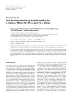
Figure 2: Comparison of histograms of P-values obtained from the
HMMs-based transition dependency and the dynamic correlation.

The sample dynamic correlation for the simulated data
depicted in Figure 1 is −0.006, indicating no linear correlation between the two processes. In contrast, the Kronecker
product of two marginal transition probabilities is given by
0.2475
0.3025
0.2025
0.2475

0.8

150

Frequency

It is easy to show that the stationary distribution of the
resulting Markov process is π = (0.25, 0.25, 0.25, 0.25),
which leads to an expected zero value of the dynamic
correlation between the two marginal processes X1· and X2· .
Therefore, the dynamic correlation will not be able to detect
any dependency between these two processes. As a matter
of fact, the two-time series mutually influence each other
in order to reach an equilibrium state. That is, if they are
both in DR or both in UR, they tend to remain at the same
state; if not, say, one of them being in DR and the other
in UR, then they tend to induce the DR gene and suppress
the UR gene. This type of biological regulation for achieving
and maintaining the equilibrium state is often observed
between RNA upstream and downstream configurations
[15]. Figure 1 displays two simulated trajectories according

to the given joint transition matrix (2).

0.3025
⎢0.2475
⎢
⎢
⎣0.2475
0.2025

1

(a) HMMs method

Figure 1: Simulated expression status of RNA upstream and
downstream configurations.

⎡

0.8

a

⎤

0.2025
0.2475⎥
⎥
⎥.
0.2475⎦
0.3025

e

c

b

(3)

It is evident that there is a large discrepancy between the
joint transition matrix (2) and the product of the marginal
transitions (3). The resulting nonzero matrix D provides the
evidence for a strong dependency between the two genes.
The failure of the traditional correlation measure to detect
the dependency here is due to the fact that it essentially
relies on the concordant and discordant changes between two
trajectories which are clearly absent in this type of nonlinear
dependency relationship.
2.2. Testing for Pairwise Dependency. Consider a statistical
test for the absence or the presence of interaction between

d

k

l

h

f

g

i
j

Figure 3: A dependency network for CD44 and its significant
relatives. Symbol “a” stands for CD44, “b” for FRMD4B, “c” for
MAPKAPK3, “d” for SOCS3, “e” for CASP8, “f ” for IDI1, “g” for
F2RL1, “h” for FAS, “i” for ANXA3, “j” for ZNF263, “k” for DnaJ,
and “l” for ENO1.


4

EURASIP Journal on Bioinformatics and Systems Biology

two genes. The null hypothesis is H0 : D = 0, where 0 is a
4 × 4 matrix of all elements equal to zero. Pearson-type χ 2
test is popular to test for independence, and our proposed
test will follow on this line. As a first step to construct a
test statistic, we need to obtain the maximum likelihood
estimate (MLE) for the transition matrix. Assume there are
M replications of the observed data Yi , i = 1, . . . , M, with
i
i
Yi = (Yi·t , t = 1, . . . , T), and Yi·t = (Y1,t , Y2,t ), where the first
subscript indexes for the observations of gene 1 and gene 2,
and the second subscript indexes for the time point. Let V =
{(0, 0), (0, 1), (1, 0), (1, 1)} denote the set of four possible

i
i
i
configurations of the joint hidden states for X·t = (X1,t , X2,t ).
Denote the distribution of the bivariate state vector at the
i
initial time by p = (p j ), with p j = P(X·1 = v j ), v j ∈ V, j =
1, 2, 3, 4. Then, the augmented likelihood of the “complete”
data with a given transition matrix takes the following form:
M

Li (Λ, p; Yi , Xi )
i=1
M

4

=

i
I(X·1 =v j )

pj
i=1

t =1

j =1

×

T −1

i
X1,t

ft

i
X2,t

i
(Y1,t ) ft

4
i
(Y2,t )

i
i
I(X·t =v j ,X·t+1 =vk )

Λ jk
j,k=1

Xi

Xi

i

i
× fT 1,T (Y1,T ) fT 2,T (Y2,T ) .

(4)
The maximum likelihood estimates of the unknown parameters θ = (Λ, p) can be obtained as
M

log Li (Λ, p; Yi , Xi )dXi .

θ = (Λ, p) = argmax
θ

(5)

i=1

i
As the hidden state vectors X·t are unobserved, the EM
algorithm is invoked to carry out the maximum likelihood
estimation, which iterates the following two steps till convergence.

E Step: given θ old , we calculate two conditional expectations that are the expected numbers of transitions:
i
i
i
E{I(X·t = v j , X·t+1 = vk ) | Yi , θ old } = P(X·t =
i
i , θ old ), and E{I(Xi = v ) |
v j , X·t+1 = vk | Y
j

·t
i
Yi , θ old } = P(X·t = v j | Yi , θ old ). This is achieved
by using the forward-backward algorithm especially
designed for the HMMs model [16].
M Step: given these expected numbers of transitions
between the states, we update the transition matrix
by the following MLE:
Λnew =
jk

M
i=1

M

pnew
j

T −1
i
i
i old
t =1 P(X·t+1 = vk , X·t = v j | Y , θ )
,
M
T −1
i
i old
i=1

t =1 P(X·t = v j | Y , θ )

1
i
=
P(X·1 = v j | Yi , θ old ).
M i=1

(6)

As usual, multiple starting points can be used to achieve
the global maximum instead of local stationary points. To
test for the null hypothesis H0 , we can tabulate relevant
data in a form of contingence table, where cell count n jk
denotes the total number of transitions between states v j
and vk . Let a( j1 , k1 ) be the number of marginal transitions
from X1,t = j1 to X1,t+1 = k1 for gene 1, and let b( j2 , k2 )
be the number of marginal transitions from X2,t = j2 to
X2,t+1 = k2 for gene 2, with j1 , k1 , j2 , k2 = 0, or 1. Under
the H0 , the expected frequency of transitions is EH0 (n jk ) =
a(v j [1], vk [1])b(v j [2], vk [2])/M(T − 1), where v j [s] denotes
the sth element of vector v j , s = 1, or 2. Thus a chisquared-type test statistic [17] can be formed as χ 2 =
2
j k {n jk − EH0 (n jk )} /EH0 (n jk ).
Even when the ni j s are available, because of the autocorrelations between the transitions across time points, the
limiting distribution of χ 2 is not a chi-squared distribution
of 9 degrees of freedom. Furthermore, all the counts n jk
are not observed, we have to estimate them. Upon the
convergence of the EM algorithm, we may obtain the
estimated counts of transitions between each pair of states:

−
i
i
n jk = M 1 T=11 P(X·t = v j , X·,t+1 = vk | Yi , Λ, p), j, k =
i=
t
1, . . . , 4. The resulting statistic is denoted by χ 2∗ , with n jk in
place of ni j in the χ 2∗ statistic. Thus the estimation procedure
brings extra random variation into the statistic χ 2∗ .
To assess the significance of χ 2∗ statistic, we invoke the
bootstrap method to generate its empirical null distribution.
We randomly resample the bivariate hidden Markovian
process under the null hypothesis (cross-independence) as
follows. From the EM algorithm, we estimate the marginal
transition matrices under the null hypothesis. For each run
of bootstrap sampling, using p j , and the estimated marginal
transition matrices, we randomly generate M bivariate
Markovian processes where the two processes of hidden
states are cross-independent. Based on the sample path of
i
the X·t , we then randomly generate the measurement process
i
Y·t according to the conditional distributions. Subsequently,
i
we discard X·t , treat the generated Yi·t as the bootstrap data,
and invoke the EM algorithm. Utilizing the output of the
EM estimates based on the bootstrap data, we can calculate
a value of χ 2∗ statistic, which can be viewed as a random
draw from the null distribution of the statistic. By generating
a large number of bootstrap replicates, we can obtain the

empirical distribution of the null statistic which provides
an accurate approximation to the null distribution of χ 2∗
statistic.
2.3. Pairwise Analysis. In microarray data, the expression
trajectories of N genes can be modeled as an N-variate times
i
series data, Y = {Yn,t , i = 1, . . . , M, n = 1, . . . , N, t =
1, . . . , T }, where i indexes for the sample replicate, n indexes
for the nth variate (gene), and t indexes for the time point. In
practice, two kinds of pairwise analyses may be considered:
(1) given a specific gene of interest, and the task is to infer all
the genes that interact with this gene; (2) test all N(N − 1)/2
pairs exhaustively, and select the most significant pairwise
dependencies for a further analysis.
In both scenarios, a list of potentially promising interactions are determined while the false discovery rate (FDR) is


EURASIP Journal on Bioinformatics and Systems Biology

5

Table 1: Empirical type I error rates and power of the proposed bootstrap-based (BS) χ 2∗ test versus the dynamic correlation (DC) and
cross-correlation function (CCF) to detect pairwise dependency under the dependency pattern I. The power refers to the probability of
detecting the interaction when the interaction really exists. The symbol B denotes the number of bootstrap samples generated for each gene.
The symbol d denotes the deviation parameter.

Replicates

Time points

2

7

2

10

3

7

3

10

5

7

5

10

d
0.00
0.05
0.10
0.15
0.00

0.05
0.10
0.15
0.00
0.05
0.10
0.15
0.00
0.05
0.10
0.15
0.00
0.05
0.10
0.15
0.00
0.05
0.10
0.15

BS-χ 2∗
0.084
0.135
0.249
0.472
0.054
0.131
0.281
0.583
0.071

0.118
0.302
0.594
0.049
0.163
0.401
0.766
0.056
0.172
0.488
0.822
0.042
0.231
0.624
0.946

under control. False discovery rate (FDR) is an error measure
used in the context of multiple hypotheses testing. Given a
family of L simultaneously tested null hypotheses of which
L0 are true. Let R denote the number of rejected hypotheses,
and let V denote the number of true hypotheses erroneously
rejected. Let Q denote V/R when R > 0, and 0 otherwise.
Then the FDR is defined as FDR = E(Q), the expected rate
of false discovery. As shown in [18], the FDR of a multiple
comparison procedure is always smaller than or equal to
the familywise error rate (FWER). To control the FDR, we
proceed as follows. For each pair (n, n ), we construct the
2∗
χn,n test statistic, and also generate bootstrap-based null
2∗

statistics χ0;n,n . To deal with the issue that test statistics are
correlated, we follow Reiner et al. [19] to form the null
distribution by collapsing all the null statistics together. Thus
the P-value of each pairwise test can be obtained by referring
to the empirical null distribution. Given the ordered Pvalues, p(1) ≤ · · · ≤ p(L) , the multiplicity adjusted P-value
employed by the Benjamini-Hochberg (BH) procedure [18]
(BH)
is pk = mins≥k (p(s) L/s), where L denotes the total number
of tests under screening. Pairs with adjusted P-values less
than a prespecified FDR are declared to be significant and
selected for a further consideration. Although this screening

B = 20
DC
0.057
0.092
0.198
0.388
0.053
0.101
0.256
0.561
0.055
0.120
0.284
0.586
0.058
0.131
0.388
0.735

0.051
0.141
0.478
0.823
0.070
0.196
0.648
0.938

B = 30
DC
0.054
0.077
0.183
0.369
0.045
0.113
0.286
0.561
0.053
0.109
0.288
0.567
0.052
0.127
0.384
0.732
0.050
0.133
0.452

0.841
0.038
0.198
0.647
0.953

BS-χ 2∗
0.070
0.120
0.260
0.448
0.044
0.118
0.298
0.577
0.058
0.127
0.313
0.564
0.060
0.133
0.396
0.754
0.060
0.165
0.468
0.843
0.054
0.218
0.638

0.949

CCF
0.038
0.038
0.061
0.098
0.049
0.052
0.081
0.150
0.043
0.056
0.109
0.168
0.042
0.072
0.123
0.253
0.036
0.073
0.155
0.298
0.051
0.087
0.227
0.456

CCF
0.039

0.045
0.073
0.092
0.033
0.045
0.100
0.157
0.051
0.058
0.110
0.144
0.059
0.061
0.135
0.256
0.037
0.066
0.153
0.294
0.052
0.083
0.260
0.463

procedure potentially contains some false positives, it is
computationally efficient and provides a promising pool of
candidate relationships for a future analysis.

3. Results on Simulated Data
A simulation study was conducted to investigate the empirical performance of the proposed bootstrap-based test for

pairwise gene dependency. One thousand pairs of genes were
simulated under different transition probabilities. Under
the null hypothesis H0 of independence, the underlying
transition matrix takes the form
⎡

a1 b1
⎢a b
⎢ 1 3
H0 : Λ0 = ⎢
⎣a3 b1
a3 b3

a1 b2
a1 b4
a3 b2
a3 b4

a2 b1
a2 b3
a4 b1
a4 b3

⎤

a2 b2
a2 b4 ⎥
⎥
⎥,
a4 b2 ⎦

a4 b4

(7)

where the parameters satisfy a2 = 1 − a1 , a4 = 1 −
a3 , b2 = 1 − b1 , b4 = 1 − b3 , and a1 ∼ U(0.4, 0.6),
a3 ∼ U(0.4, 0.6), b1 ∼ U(0.4, 0.6), b3 ∼ U(0.4, 0.6), with U
denoting a uniform distribution. To specify the alternative
hypothesis, we considered a deviation drift d, which deviates


6

EURASIP Journal on Bioinformatics and Systems Biology

Table 2: Empirical type I error rates and power of the proposed bootstrap-based (BS) χ 2∗ test versus the dynamic correlation (DC) and
cross-correlation function (CCF) to detect pairwise dependency under the dependency Pattern II. The power refers to the probability of
detecting the interaction when the interaction really exists. The symbol B denotes the number of bootstrap samples generated for each gene.
The symbol d denotes the deviation parameter.

Replicates

Time points

2

7

2

10

3

7

3

10

5

7

5

10

d
0.00
0.05
0.10
0.15
0.00
0.05
0.10
0.15
0.00
0.05
0.10

0.15
0.00
0.05
0.10
0.15
0.00
0.05
0.10
0.15
0.00
0.05
0.10
0.15

B = 20
DC
0.057
0.048
0.053
0.046
0.053
0.050
0.047
0.049
0.052
0.048
0.057
0.037
0.054
0.050

0.048
0.045
0.049
0.055
0.058
0.053
0.049
0.058
0.044
0.058

BS-χ 2∗
0.084
0.077
0.078
0.125
0.059
0.087
0.086
0.152
0.059
0.085
0.106
0.137
0.049
0.081
0.116
0.222
0.065
0.073

0.131
0.203
0.042
0.094
0.186
0.475

the null transition matrix Λ0 according to the following two
patterns: Pattern I takes the form
⎡

a1 b1 + d
⎢a b + d
⎢ 1 3
(1)
H1 : Λ1 = ⎢
⎣a3 b1 + d
a3 b3 + d

a1 b2 − d
a1 b4 − d
a3 b2 − d
a3 b4 − d

a2 b1 − d
a2 b3 − d
a4 b1 − d
a4 b3 − d

⎤

a2 b2 + d
a2 b4 + d ⎥
⎥
⎥,
a4 b2 + d ⎦
a4 b4 + d
(8)

and Pattern II takes the form
⎡

a1 b1 + d
⎢a b − d
⎢ 1 3
(2)
H1 : Λ2 = ⎢
⎣a3 b1 − d
a3 b3 + d

a1 b2 − d
a1 b4 + d
a3 b2 + d
a3 b4 − d

a2 b1 + d
a2 b3 − d
a4 b1 − d
a4 b3 + d

⎤

a2 b2 − d
a2 b4 + d ⎥
⎥
⎥.
a4 b2 + d ⎦
a4 b4 − d
(9)

In our simulation study, a few scenarios were given via the
combinations of different parameter values, including the
deviation parameter d = 0.05, 0.10, and 0.15, the number
of replicates M = 2, 3, and 5, and the number of time
points T = 7 and 10. For each pair of genes, 20 or 30
bootstrap samples were generated to form the null statistics,
and they were then collapsed together to form the empirical
null distribution [19]. The conditional distributions ft0 and

CCF
0.038
0.036
0.045
0.038
0.047
0.040
0.032
0.039
0.028
0.045

0.052
0.031
0.041
0.042
0.037
0.036
0.035
0.044
0.044
0.052
0.048
0.058
0.054
0.042

BS-χ 2∗
0.076
0.066
0.095
0.122
0.058
0.063
0.102
0.157
0.074
0.070
0.099
0.137
0.045
0.051

0.126
0.217
0.059
0.071
0.114
0.239
0.052
0.064
0.181
0.516

B = 30
DC
0.038
0.051
0.059
0.044
0.033
0.039
0.043
0.048
0.045
0.049
0.052
0.053
0.041
0.047
0.040
0.043
0.056

0.057
0.050
0.049
0.049
0.045
0.041
0.060

CCF
0.032
0.042
0.041
0.038
0.039
0.043
0.040
0.037
0.040
0.042
0.040
0.041
0.045
0.043
0.032
0.051
0.050
0.051
0.043
0.039
0.047

0.040
0.049
0.054

ft1 were chosen to be N(0, 1), and N(4, 1), respectively.
To test the null hypothesis H0 , our HMMs approach was
compared with two correlation-measure-based methods,
namely, the sample dynamic correlation (DC) method and
the classical cross-correlation function (CCF) method in the
theory of multivariate time series analysis. Both DC and CCF
methods used their respective empirical distribution from
the bootstrap samples to obtain the corresponding P-values
under the null hypothesis H0 .
Tables 1 and 2 provide the empirical type I error rates
and the power of these three competing methods under the
two different dependency patterns over 1000 simulations.
Type I error rates given by all the three methods (with d =
0) were reasonably controlled at the 0.05 level. Comparing
the power across these three methods, we can see that the
bootstrap-based χ 2∗ test (BS-χ 2∗ ) clearly outperformed the
(1)
other two methods. Under the alternative H1 of Pattern
I, the BS-χ 2∗ method maintained fairly satisfactory power,
which was always better than the two correlation-measure(2)
based methods. Under the alternative H1 of Pattern II, it
is interesting to see that the two correlation-measure-based
methods had no power of detecting the dependency here.
Their power values were constantly around 0.05, regardless

EURASIP Journal on Bioinformatics and Systems Biology

7

CDK4

TRAF5

CD69

TCF12

CASP8

RB1

CYP19

E2F4

APC

PIG3

TCF8

CSF2RA

CCNG1

IRAK1

PDE4B

JUNB

MAPK9

SIVA

IL3RA CDC2

CASP7

SKIIP

MCL1

CCNC

PCNA

MYD88

API2

C3X1

JUND

CLU

MAP3K8

SOD1

CCNA2 SMN1

IFNAR1 RBL2

CIR

EGR1

LCK

SLA

IL16

MPO

AKT1

GATA3

FYB

IL2RG

NFKBIA

Figure 4: A major dependency network of 58 genes in T-cell data analysis.

Table 3: The list of the15 most significant candidate genes having interactions with CD44.
Probe
38336 at
947 at
39237 at
40968 at
31491 s at
36985 at
36344 at
1441 s at
31792 at
33289 f at
953 g at
35799 at
2035 s at
31318 at
296 at

pcorr
0.00110891
0.04692277
0.51548517
0.00367525
0.00107723
0.02434851
0.01527129

0.01954851
0.00267723
0.00365941
0.01698218
0.02151287
0.00327921
0.03653069
0.03504159

phmm
9.505e − 05
0.00011089
0.00017426
0.00017426
0.00019010
0.00020594
0.00022178
0.00023762
0.00023762
0.00023762
0.00023762
0.00025347
0.00026931
0.00028515
0.00030099

Gene title
FERM domain containing 4B (FRMD4B)
Gene function unknown
Mitogen-activated protein kinase 3 (MAPKAPK3)

Suppressor of cytokine signaling 3 (SOCS3)
Caspase 8 (CASP8)
Isopentenyl-diphosphate delta isomerase (IDI1)
Coagulation factor II (thrombin) receptor-like 1 (F2RL1)
Tumor necrosis factor receptor superfamily, member 6 (FAS)
Annexin A3 (ANXA3)
Zinc finger protein 263 (ZNF263)
Gene function unknown
DnaJ (Hsp40) homolog, subfamily B, member 9 (DNAJB9)
Enolase 1, (alpha) (ENO1)
Gene function unknown
Gene function unknown

of the size of dependency (i.e., deviation d). In contrast, the
power of the BS-χ 2∗ method responded well to the increase
in deviation d.
Why did the two correlation-measure-based methods
perform well under the dependency Pattern I, but very
poorly under Pattern II? This is because the correlation essentially measures the discordance and concordance
between the joint expression states. For example, given
the transition matrix under the null distribution specified
by a1 = 0.48, a3 = 0.51, b1 = 0.40, b3 = 0.55,

Literature
[21]
[22]
[23]
[24]

[25]

[26]

[27]

when the deviation d increases from 0.1 to 0.15, the
i
i
stationary distribution of (X1,t , X2,t ) on the four possible pairs (0, 0), (0, 1), (1, 0), and (1, 1) will change from
(0.32, 0.14, 0.15, 0.37) to (0.37, 0.09, 0.10, 0.42) under Pattern
I. Apparently, such a stationary distribution allocates more
probabilities on the concordance pairs (0, 0), namely 0.32
and 0.37, and (1, 1), namely 0.37 and 0.42. This causes high
correlation easy to detect. In contrast, Pattern II behaves
strikingly different. When d increases from 0.1 to 0.15,
i
i
the stationary distribution of (X1,t , X2,t ) remains almost the


8

EURASIP Journal on Bioinformatics and Systems Biology

16

Value

0

18

16

CD69

•
•
•
•
•
•

•
•
•
•
•

•
•
•
•

•
•
•
•
•

20
18

16

10

20

30
40
Time

50

60

70

•
•

•
•
•
•
•

•
•
•
•
•

10

20

•
•
•
•
•

•
•
•
•
•

•
•
•
•
•
•
•

0

30
40
Time

50

60

18

70

10

16

Value

0

17
16

•
•
•
•
•

•
•
•
•

•
•

Value

•
•
•
•
•

18.5

17
10

•
•
•• •
•• •
•
•••••
•••••
•
•••••
• •
••••
••
•••••
•••

•
••

0

•
•
•
•
•
•
•

10

20

30
40
Time

50

60

70

•
•

•
•
•
•
•
•
•

•
•
•
•
•
•
•
•
20

30
40
Time

50

60

70

EGR1

10

•
•
•

•
•
•

•
•
•
•

•
•
•
•
•

20

30
40
Time

50

60

70

•
•
•
•
•
•
•
•
•

•
•
•
•
•
•
•
•

20
18

60

70

(c) Nonlinear

•
•
•
•
•
•
•
•
•

•
•
•
•
•
•
•
•
•
•
•
•

10

20

•
•

•
•
•
•
•
•
•

•
•
•
•
•
•
•
•
•

•
•
•
•
•
•
•
•

30
40
Time

50

60

70

FYB

••
••
•••
••• •
• •
•••
•••
•

•
•
•

•
•
•

•
•

•

•

•
•
•

•

16
50

CCNC

• •
•
•
•••••
•••••
•••••
•• •
••••
•
••••
• •
••••
•• •
•
••
0

PDE4B

•
•
•
•
•
•
•
•

30
40
Time

•
•
•
•
•

(b) Coexpression

E2F4

•
•
•
•
•

•

•
•
•
•
•
•

•
•
•
•
•
0

Value

Value

17.5

•
•
•
•

20

•

•
•

(a) Inverted

• •
• • •
••• •
• •
•••••
•
•••••
•••••
•
•• •
•
•
•

•
•
•
•
•

•
•
•
•

••••
••••
•••
• •
•

20

16

JUND

•
•
••••
••••
• ••
• •
•
• •
•
• •

TCF12

•
••
•••
•
•••••

••••
•
••• •
•• •
•••
•••
0

•
•
•
•
•

•
•
•
•

Value

18

•
• •
•••
••••
• •
••••
••

••••
•••
•
•
•

Value

Value

20

0

10

20

30
40
Time

50

60

70

(d) Nonlinear

Figure 5: Examples of pairwise time series identified to have interactions. Each panel contains the time series plots, with dots representing
observed replicated expression levels, and solid lines representing the average expression level across time points.

same, from (0.22, 0.24, 0.25, 0.27) to (0.22, 0.24, 0.25, 0.27).
The stationary distribution takes almost equal probabilities
on these four pairs. The evenly distributed concordant and
discordant pairs lead to low correlations. This explains the
poor power of the correlation-measure-based methods to
detect dependency Pattern II.

4. Results on Biological Data
4.1. Apoptosis Data Analysis. To investigate the practical
performance of the proposed method, we consider the neutrophil apoptosis microarray dataset produced by Kobayashi
et al. [20]. The neutrophils are important cellular component
of the innate immune system in humans. It is essential that
neutrophils undergo spontaneous apoptosis as a mechanism
to facilitate the stability of the immune system. To get a
global view of the molecular events that regulate neutrophil
survival and apoptosis, Kobayashi et al. [20] studied the
global expression in human neutrophils during spontaneous

apoptosis cultured with and without human GM-CSF, which
is known to prolong neutrophils survival against apoptosis.
Neutrophils were isolated from venous blood of three healthy
individuals and were cultured in the medium with and
without 100 ng/mL GM-CSF for up to 24 hours. At time
points, 3 hours, 6 hours, 12 hours, 18 hours, and 24 hours,
the expression level of 12 625 genes were measured using
GeneChip hybridization technique. The time course data we
analyzed contains 30 samples comparing treatment (+GMCSF) versus control (−GM-CSF) at the corresponding 5time points in three biological replicates.

To use this dataset and understand the gene regulatory
network, as a first step, we wish to find out how genes are
interacting with each other. We selected CD44 as our gene of
interest and set out to find all the genes that are interacting
with CD44 during the neutrophils apoptosis. CD44 is an
important gene which encodes a cell surface glycoprotein
involved in cell-cell interactions, cell adhesion and migration. This protein participates in a wide variety of cellular


EURASIP Journal on Bioinformatics and Systems Biology
functions including lymphocyte activation, recirculation and
homing, hematopoiesis, and tumor metastasis. It is expected
that CD44 interacts with a variety of genes to facilitate
its various functions. Furthermore, CD44 is an important
tumor marker which is released by cancerous cells and could
be detected by blood tests to detect the presence of cancer. To
provide a list of candidate genes which interact with CD44
can provide more insight into the biological mechanism
underlying tumor progression.
i
To apply the proposed HMMs, we first took Yn,t to be
the absolute difference between the ith biological replicate’s
expression levels under the two experiment conditions from
gene n evaluated at time t. Next we need to determine
the conditional distributions ft0 (y), and ft1 (y) given the
NDE status and DE status. Nonparametric empirical Bayes
method in [11] was employed to estimate these conditional
distributions, both of which were fixed in all the subsequent
hypothesis tests for computational convenience. It assumes
i

that the underlying distribution for the statistic Yn,t , i =
1, . . . , M, n = 1, . . . , N, is a mixture distribution containing
two components: f t = π0 f0t + π1 f1t , where f0t , f1t represent
the components corresponding to DE state (0) and NDE
state (1), and π0 and π1 are the probability that an observed
y is sampled from f0t and f1t , respectively. Then based on
i
Yn,t , one can make posterior inference whether the specific
observation is from state (0) or state (1). Unlike the classical
Bayes approach, which assumes specific parametric forms of
f0t and f1t , the nonparametric empirical Bayes uses the data to
estimate the densities of f0t , and f1t . First the data is randomly
permuted across the two-sample experimental conditions
and the null statistic is generated. By a great number of
permutations, we could obtain a large random sample from
f0t . Therefore, we can estimate the densities of both f t and f0t
using nonparametric methods, such as the kernel estimation.
The gene-gene interaction was examined by testing for
independence between CD44 and each of the remaining
12 624 genes. As all the test statistics are related to the
expression data of CD44, all the 12 624 test statistics are not
independent. To adjust for the multiplicity of the test statistics with high intercorrelations, the resampling-based FDR
control method discussed above was employed. Bootstrap
samples were generated to get the null distribution of the test
statistics and the null statistics were collapsed to assess the Pvalues of the test statistics under the dependency structure.
Then the P-values were adjusted for the multiplicity through
the BH procedure. The significant genes were selected while
maintaining the FDR control at the level of 0.1. We detected
302 significant genes having interactions with CD44 among
the remaining 12 624 genes. Table 3 provides the list of the

most significant 15 genes having interactions with CD44,
including gene names, gene functions, and the P-values.
Some of these genes have existing biological evidence to
directly support our findings, while some other genes have
indirect evidence about the interaction between CD44 and
relevant genes encoding proteins in the same protein family.
Related references are included in the table as well.
The results of the HMMs and the dynamic correlation
methods are in agreement in most cases but differ in some
cases. For the example of the third most significant gene

9
MAPKAPK3, the estimated expected transition matrix under
the null hypothesis is
⎡

0.31
⎢0.22
⎢
⎢
⎣0.22
0.15

0.25
0.34
0.17
0.24

0.25
0.17

0.34
0.24

⎤

0.19
0.27⎥
⎥
⎥,
0.27⎦
0.38

(10)

and the estimated joint transition matrix is
⎡

0.56 1.171 × 10−8 1.30 × 10−3
⎢0.71
0.04
0.04
⎢
⎢
⎣0.88 1.66 × 10−11 4.50 × 10−7
0.39 1.46 × 10−4 1.45 × 10−4

⎤

0.44
0.21⎥

⎥
⎥.
0.12⎦
0.61

(11)

The resulted χ 2∗ test statistics is 35.90 and the P-value is
1.74 × 10−4 . The strong dependency between the genes CD44
and MAPKAPK3 is revealed by the big discrepancy between
the expected and the actual transition matrices. The joint
state of the two genes has much smaller probability than
expected to transit to states (0, 1) and (1, 0). In comparison,
the estimated Pearson’s correlation is only 0.18 with the
insignificant P-value of 0.52.
It is worthy to highlight our findings of the significant
interaction between CD44 and caspase 8. Our method ranks
caspase 8 as the fifth in the list with a P-value of 1.90 × 10−4
whereas, the dynamic correlation method ranks caspase 8
as the 308th in the list with a P-value of 1.08 × 10−3 . The
transition dependency matrix D was estimated to be
⎡

0.24 −0.24
⎢0.55 −0.28
⎢
⎢
⎣0.50 −0.19
0.22 −0.22

⎤
−0.24 0.24
−0.19 −0.07⎥
⎥
⎥.
−0.28 −0.03⎦
−0.22 0.22

(12)

The signs of the entries significant away from zeros are
⎡

+ − −
⎢+ − −
⎢
⎢
⎣+ − −
+ − −

⎤

+
.⎥
⎥
⎥.
.⎦
+

(13)

This dependency pattern is very similar to Pattern I considered in our simulation. It implies that caspase 8 and CD44
are involved in the same pathway of apoptosis and they
tend to be in the same states of DE or NDE, depending on
whether the pathway is initiated or not. This discovery only
informs us about the existence of dependency but does not
provide information about the physical mechanism. Searching through the literature, we found that this dependency is
caused by the event that the CD44 encoded protein ligates
with A3D8, acts as a transcription factor, and initiates the
transcription of caspase 8 [24]. This discovery is of great
biological implication in the sense that it unveils a new
apoptosis pathway and sheds light to a potential therapeutic
drug—A3D8 which ligates to CD44 and initiates caspase 8
in the pathway—to treat leukemia patients who are resistant
to traditional chemotherapy agents ATRA and As2O3. Based
solely on gene expression profiling without extensive wet lab
work, we rediscovered that gene caspase 8’s transcription


10
level is dependent on that of CD44, with stronger statistical
significance compared to the dynamic correlation method.
This demonstrates the power of the proposed method of
detecting biological meaningful dependencies.
To compare the overall performance of the HMMs
method with the correlation method, we plotted the histograms (see Figures 2(a) and 2(b)) of the empirical P-values
obtained from the two methods. It is seen from Figure 2(a)
that the P-values from the HMMs method demonstrate
a sharp spike over the range of P-values less than .001.
Beyond the spike, all the remaining P-values follow an almost

uniform distribution from .001 to 1. The proportion of Pvalues less than .001 is 1.3%, whereas that less than 0.1 is
13.8%. The spike standing for 1.3 percent of the overall
genes can be roughly viewed as the collection of genes
with significant interactions with CD44, while the remaining
majority of genes is independent of CD44, belonging to the
null situation. In comparison, Figure 2(b) indicates that Pvalues from the dynamic correlation method have a much
lower degree of separation between the P-values from the
null and the alternative situations. Furthermore, there is a
large bulk of P-values less than .1, accounting for 47% of the
overall genes, whereas the percentage of P-values less than
.001 is only 0.3%. Thus, the dynamic correlation method
identifies a large proportion of genes (almost half) being
correlated with CD44 with mild statistical significance. This
excessively large proportion cannot be plausibly interrelated
to the proportion of the genes having real biological
interactions with CD44 at molecular levels. According to the
theory of sparse network held by the biologists, the HMMs
method is a more reliable method to identify a small number
of gene-gene interactions with biological significance.
We further investigated a full dependency map among
the 15 top-ranked genes. After eliminating the four probes
(947 at, 953 g at, 31318 at, 296 at) with unknown biological
functions, we relabeled the CD44 gene as gene “a”, and
the remaining 11 genes (FRMD4B, MAPKAPK3, SOCS3,
CASP8, IDI1, F2RL1, FAS, ANXA3, ZNF263, DnaJ, ENO1)
in the list as “b” to “l”. The CD44 acts as a hub connecting
to each of the remaining genes in the network. We obtained
all the pairwise test statistics (in total 55 test statistics for
11 genes) in the network and calculated the corresponding
P-values via the bootstrap method. Based on the individual

P-value threshold of P < .0003, which corresponds to the
familywise type I error rate controlled at 0.02, our analysis
yields a dependency network consisting of 12 nodes and 19
edges, shown in Figure 3. In the graph, an edge linking two
genes demonstrates a significant dependency between them,
whereas the absence of an edge means there is no significant
dependency relationship between the two genes. Among the
19 edges in the network, 10 edges are supported by the
existing biological evidence. According to Cheng et al. [28],
there is a positive feedback loop that couples Ras/MAPK
activation which involves MAPKAPK3 (node c) and CD44
(node a) alternative splicing. The presence of SOCS3 (node
d) acts as a negative feedback on the activity of signaling
in the JAK/STAT pathway [29], which involves ANXA3
(node i). Furthermore, the JAK/STAT pathway crosses with
the Ras/MAPK pathway at multiple levels, each enhancing

EURASIP Journal on Bioinformatics and Systems Biology
activation of the other [30]. Based on these biological results,
we conclude that the selected network actually reflects how
the three pathways—Ras/MAPKAPK3 signaling pathway,
JAK/STAT signaling pathway, and caspase-dependent apoptosis pathway—interconnect with each other through the
hub gene CD44.
4.2. T-Cell Data Analysis. We also analyzed the T-cell
data [31] to study the genetic dependency network in
the activation process of T-cells. To generate an immune
response, the T-cells become activated and then proliferate,
and produce cytokines involved in the regulation of B cells
and macrophages, which are the most important mediators
of the immune response. It is known that T-cell activation is

initiated by the interaction between the T-cell receptor complex and the antigens. This stimulates a network of signaling
molecules, including kinases, phosphatases, and adaptor
proteins that parallel the stimulatory signals received by the
nucleus to control the gene transcription events. The calcium
ionophore ionomycin and the PKC activator phorbol ester
PMA were used to activate signaling transduction pathways
leading to T-cell activation. Microarray measurements of
58 genes which are relevant to the immune response were
taken at the following times after the treatment: 0, 2, 4,
6, 8, 18, 24, 32, 48, and 72 hours. For each time point,
there are 44 replicated measurements for each gene. This
dataset is different from the previous apoptosis data as it is
one-sample data with only one experimental condition. We
used a mixture of two Gaussian distributions to model the
distribution of the expression level for each gene, conditional
on downregulated or upregulated state. In the pairwise
analysis, we screened all possible pairs of genes exhaustively
and constructed a complete dependency map for these 58
genes. For each pair, B = 100 bootstrap samples were
generated to facilitate the assessment of P-values. A major
network is obtained, consisting of 47 genes out of the total
58, in which 89 edges have P-values significant at the .003
level. The network is shown in Figure 4.
We further examined all the pairwise time series corresponding to the selected edges, some examples are shown in
Figure 5. From their time series plots, we noticed that our
method was capable of identifying many different patterns.
The patterns include coexpression, where the two time series
follow the same trend of going up or down. Another pattern
is inverted, where the two time series show opposite changes
over time. There exist other scenarios, where the two time

series do not obey any obvious linear patterns, indicating the
nonlinear combinatorial dependency relationships between
the two genes. In comparison, existing methods like the
linear dynamic system or the Gaussian graphical model are
unable to identify such patterns.

5. Discussion
Detecting gene-gene interaction is one of the most important
tasks in the study of system biology. The advent of time
series microarray data challenges statisticians to develop a
statistical machinery to extract and summarize the dependency information embedded in the data. In this paper,


EURASIP Journal on Bioinformatics and Systems Biology
we characterize the dependency relationships based on the
dynamics of a hidden Markov model, so that we are able
to monitor the gene-gene interactions through transitional
probabilities. The proposed methodology is not restricted
to the microarray dataset we focus on in this article.
It can be viewed as a general approach to analyze time
series data with complicated dependency structure, such as
brain image data and proteomics data. The method can
be extended in a few directions. One limitation of the
proposed method is the assumption of stationarity on the
hidden process. This is more constrained by the practical
limitations of small replications of microarray data rather
than theoretical considerations. If the number of replications
at each time point is greatly increased, we could relax the
homogeneous assumption and model different transition
kernels at different time points.

As requested by one of the referees, we compare our
method and other existing methods in this concluding
paragraph, highlighting the advantages and limitations of
each method. Dynamic Bayesian networks (DBNs) have
been proposed to infer directed graphs from time series
data [32]. This method maximizes the Bayesian scoring
function over alternative network models. A prior knowledge
or assumption of the hierarchical structure is needed.
Furthermore, it is computationally prohibitive to go through
all the possible models as the cardinality of the model space
grows exponentially with the number of genes. Therefore,
the DBNs method is not capable of handling large networks.
Linear dynamic system is also proposed [31] to model
gene networks based on time series data. It is essentially a
linear autoregressive model allowing extra hidden variables.
It assumes the linear relationship between genes which may
not be tenable in practice. In contrast, our method focuses
on exploring pairwise dependencies between the genes.
The computational complexity is much less demanding
than the DBNs method. This enables us to analyze much
larger datasets than the DBNs method. Compared to linear
dynamic system method, our method can model nonlinear
and combinatorial relationships among genes, which is more
realistic than the linear assumptions. In conclusion, the
computational simplicity in the algorithm, the capability
of handling large dataset, modeling nonlinear relationships,
and no prior assumptions of the network structure are the
advantages of our method. Nevertheless, the limitation of
our method is that it only produces undirected graph. In
practice, our method can be used as the first screening

method to identify the potential candidate edges. Once we
narrow down our candidate genes list to a small set, we
can use the DBNs method to study a finer structure of the
network with additional details such as directions.

Acknowledgment
This research was supported by the Natural Sciences and
Engineering Research Council of Canada Grant.

References
[1] E. Alm and A. P. Arkin, “Biological networks,” Current
Opinion in Structural Biology, vol. 13, no. 2, pp. 193–202, 2003.

11
[2] J. Zhang, Y. Ji, and L. Zhang, “Extracting three-way gene
interactions from microarray data,” Bioinformatics, vol. 23, no.
21, pp. 2903–2909, 2007.
[3] H. Nakahara, S.-I. Nishimura, M. Inoue, G. Hori, and S.-I.
Amari, “Gene interaction in DNA microarray data is decomposed by information geometric measure,” Bioinformatics, vol.
19, no. 9, pp. 1124–1131, 2003.
[4] M. B. Eisen, P. T. Spellman, P. O. Brown, and D. Botstein,
“Cluster analysis and display of genome-wide expression
patterns,” Proceedings of the National Academy of Sciences of
the United States of America, vol. 95, no. 25, pp. 14863–14868,
1998.
[5] S. Tavazoie, J. D. Hughes, M. J. Campbell, R. J. Cho, and
G. M. Church, “Systematic determination of genetic network
architecture,” Nature Genetics, vol. 22, no. 3, pp. 281–285,
1999.
[6] Y. Ji, C. Wu, P. Liu, J. Wang, and K. R. Coombes, “Applications

of beta-mixture models in bioinformatics,” Bioinformatics, vol.
21, no. 9, pp. 2118–2122, 2005.
[7] J. A. Dubin and H.-G. Mă ller, Dynamical correlation for
u
multivariate longitudinal data, Journal of the American Statistical Association, vol. 100, no. 471, pp. 872–881, 2005.
[8] L. D. Haugh, “Checking the independence of two covariancestationary time series: a univariate residual cross-correlation
approach,” Journal of the American Statistical Association, vol.
71, no. 354, pp. 378–385, 1976.
[9] K. Basso, A. A. Margolin, G. Stolovitzky, U. Klein, R. DallaFavera, and A. Califano, “Reverse engineering of regulatory
networks in human B cells,” Nature Genetics, vol. 37, no. 4,
pp. 382–390, 2005.
[10] M. Yuan and C. Kendziorski, “Hidden Markov models for
microarray time course data in multiple biological conditions,” Journal of the American Statistical Association, vol. 101,
no. 476, pp. 1323–1332, 2006.
[11] B. Efron, R. Tibshirani, J. D. Storey, and V. Tusher, “Empirical
bayes analysis of a microarray experiment,” Journal of the
American Statistical Association, vol. 96, no. 456, pp. 1151–
1160, 2001.
[12] F. Leisch, “FlexMix: a general framework for finite mixture
models and latent class regression in R,” Journal of Statistical
Software, vol. 11, no. 8, pp. 1–18, 2004.
[13] R. L. Sandland, “Application of methods of testing for
independence between two Markov chains,” Biometrics, vol.
32, no. 3, pp. 629–636, 1976.
[14] D. Allard, A. Brix, and J. Chadoeuf, “Testing local independence between two point processes,” Biometrics, vol. 57, no. 2,
pp. 508–517, 2001.
[15] D. S. Luse and I. Samkurashvili, “The transition from
initiation to elongation by RNA polymerase II,” in Proceedings
of the 63rd Cold Spring Harbor Symposium on Quantitative
Biology (CSH ’98), B. Stillman, Ed., pp. 289–300, CSHL Press,

Cold Spring Harbor, NY, USA, June 1998.
[16] L. E. Baum, T. Petrie, G. Soules, and N. Weiss, “A maximization technique occurring in the statistical analysis of probabilistic functions of Markov chains,” Annals of Mathematical
Statistics, vol. 41, no. 1, pp. 164–171, 1970.
[17] A. Agresti, Categorical Data Analysis, John Wiley & Sons, New
York, NY, USA, 2002.
[18] Y. Benjamini and Y. Hochberg, “Controlling the false discovery
rate: a practical and powerful approach to multiple testing,”
Journal of the Royal Statistical Society. Series B, vol. 57, no. 1,
pp. 289–300, 1995.


12
[19] A. Reiner, D. Yekutieli, and Y. Benjamini, “Identifying differentially expressed genes using false discovery rate controlling
procedures,” Bioinformatics, vol. 19, no. 3, pp. 368–375, 2003.
[20] S. D. Kobayashi, J. M. Voyich, A. R. Whitney, and F. R.
DeLeo, “Spontaneous neutrophil apoptosis and regulation of
cell survival by granulocyte macrophage-colony stimulating
factor,” Journal of Leukocyte Biology, vol. 78, no. 6, pp. 1408–
1418, 2005.
[21] C.-X. Sun, V. A. Robb, and D. H. Gutmann, “Protein 4.1 tumor
suppressors: getting a FERM grip on growth regulation,”
Journal of Cell Science, vol. 115, no. 21, pp. 3991–4000, 2002.
[22] S. Weg-Remers, H. Ponta, P. Herrlich, and H. Kă nig, Regulao
tion of alternative pre-mRNA splicing by the ERK MAP-kinase
pathway,” The EMBO Journal, vol. 20, no. 24, pp. 4194–4203,
2001.
[23] A. L. Cornish, M. M. Chong, G. M. Davey, et al., “Suppressor
of cytokine signaling-1 regulates signaling in response to
interleukin-2 and other γ c-dependent cytokines in peripheral
T cells,” Journal of Biological Chemistry, vol. 278, no. 25, pp.

22755–22761, 2003.
[24] E. Maquarre, C. Artus, Z. Gadhoum, C. Jasmin, F. SmadjaJoffe, and J. Robert-L´ z´ n` s, “CD44 ligation induces apoptosis
e e e
via caspase- and serine protease-dependent pathways in acute
promyelocytic leukemia cells,” Leukemia, vol. 19, no. 12, pp.
2296–2303, 2005.
[25] K. Nakano, K. Saito, S. Mine, S. Matsushita, and Y. Tanaka,
“Engagement of CD44 up-regulates Fas Ligand expression on
T cells leading to activation-induced cell death,” Apoptosis, vol.
12, no. 1, pp. 45–54, 2007.
[26] N. R. Chintagari, N. Jin, P. Wang, T. A. Narasaraju, J. Chen,
and L. Liu, “Effect of cholesterol depletion on exocytosis of
alveolar type II cells,” American Journal of Respiratory Cell and
Molecular Biology, vol. 34, no. 6, pp. 677–687, 2006.
[27] K. A. Iczkowski, J. H. Shanks, W. C. Allsbrook, et al.,
“Small cell carcinoma of urinary bladder is differentiated from
urothelial carcinoma by chromogranin expression, absence
of CD44 variant 6 expression, a unique pattern of cytokeratin expression, and more intense γ-enolase expression,”
Histopathology, vol. 35, no. 2, pp. 150–156, 1999.
[28] C. Cheng, M. B. Yaffe, and P. A. Sharp, “A positive feedback
loop couples Ras activation and CD44 alternative splicing,”
Genes & Development, vol. 20, no. 13, pp. 1715–1720, 2006.
[29] A. Singh, A. Jayaraman, and J. Hahn, “Effect of SHP-2, SOCS3,
and PP2 on IL-6 signal transduction in hepatocytes,” in
Proceedings of American Control Conference (ACC ’06), p. 6,
Minneapolis, Minn, USA, June 2006.
[30] J. S. Rawlings, K. M. Rosler, and D. A. Harrison, “The
JAK/STAT signaling pathway,” Journal of Cell Science, vol. 117,
no. 8, pp. 1281–1283, 2004.
[31] C. Rangel, J. Angus, Z. Ghahramani, et al., “Modeling Tcell activation using gene expression profiling and state-space

models,” Bioinformatics, vol. 20, no. 9, pp. 1361–1372, 2004.
[32] B.-E. Perrin, L. Ralaivola, A. Mazurie, S. Bottani, J. Mallet,
and F. d’Alch´ -Buc, “Gene networks inference using dynamic
e
Bayesian networks,” Bioinformatics, vol. 19, supplement 2, pp.
ii138–ii148, 2003.

EURASIP Journal on Bioinformatics and Systems Biology