Evapotranspiration Remote Sensing and Modeling Part 2 docx

2
Evapotranspiration Estimation Based
on the Complementary Relationships
Virginia Venturini
1
, Carlos Krepper
1,2
and Leticia Rodriguez
1
1
Centro de Estudios Hidro-Ambientales-Facultad de Ingeniería y
Ciencias Hídricas Universidad Nacional del Litoral
2
Consejo Nacional de Investigaciones Científicas y Técnicas
Argentina
1. Introduction
Many hydrologic modeling and agricultural management applications require accurate
estimates of the actual evapotranspiration (ET), the relative evaporation (F) and the
evaporative fraction (EF). In this chapter, we define ET as the actual amount of water that is
removed from a surface due to the processes of evaporation-transpiration whilst the
potential evapotranspiration (Epot) is any other evaporation concept. There are as many
potential concepts as developed mathematical formulations. In this chapter, F represents the
ratio between ET and Epot, as it was introduced by Granger & Gray (1989). Meanwhile, EF
is the ratio of latent flux over available energy.
It is worthy to note that, in general, the available evapotranspiration concepts and models
involve three sets of variables, i.e. available net radiation (Rn), atmospheric water vapor
content or temperature and the surface humidity. Hence, different Epot formulations were
derived with one or two of those sets of variables. For instance, Penman (1948) established
an equation by using the Rn and the air water vapor pressure. Priestley & Taylor (1972)
derived their formulations with only the available Rn.
In the last three decades, several models have been developed to estimate ET for a wide

range of spatial and temporal scales provided by remote sensing data. The methods could
be categorized as proposed by Courault et al. (2005).
Empirical and semi-empirical methods: These methods use site specific or semi-empirical
relationships between two o more variables. The models proposed by Priestley & Taylor
(1972), hereafter referred to as P-T, Jackson et al. (1977); Seguin et al. (1989); Granger & Gray
(1989); Holwill & Stewart (1992); Carlson et al. (1995); Jiang & Islam (2001) and Rivas &
Caselles (2004), lie within this category.
Residual methods: This type of models commonly calculates the energy budged, then ET is
estimated as the residual of the energy balance. The following models are examples of
residual methods: The Surface Energy Balance Algorithm for Land (SEBAL) (Bastiaanssen et
al., 1998; Bastiaanssen, 2000), the Surface Energy Balance System (SEBS) model (Su, 2002)
and the two-source model proposed by Norman et al. (1995), among others.
Indirect methods: These physically based methods involve Soil-Vegetation-Atmosphere
Transfer (SVAT) models, presenting different levels of complexity often reflected in the
number of parameters. For example, the ISBA (Interactions between Soil, Biosphere, and

Evapotranspiration – Remote Sensing and Modeling
20
Atmosphere) model by Noilhan & Planton (1989), developed to be included within large
scale meteorological models, parameterizes the land surface processes. The ISBA Ags model
(Calvet et al., 1998) improved the canopy stomatal conductance and CO
2
concentration with
respect to the ISBA original model.
Among the first category (Empirical and semi-empirical methods), only few methodologies
to calculate ET have taken advantage of the complementary relationship (CR).
It is worth mentioning that there are only two CR approaches known so far, one attributed
to Bouchet (1963) and the other to Granger & Gray (1989). Even though various ET models
derived from these two fundamental approaches are referenced to throughout the chapter, it
is not the intention of the authors to review them in detail.

Bouchet (1963) proposed the first complementary model based on an experimental design. He
postulated that, for a large homogeneous surface and in absence of advection of heat and
moisture, regional ET could be estimated as a complementary function of Epot and the wet
environment evapotranspiration (Ew) for a wide range of available energy. Ew is the ET of a
surface with unlimited moisture. Thus, if Epot is defined as the evaporation that would occur
over a saturated surface, while the energy and atmospheric conditions remain unchanged, it
seems reasonable to anticipate that Epot would decrease as ET increases. The underlying
argument is that ET incorporates humidity to the surface sub-layer reducing the possibility for
the atmosphere to transport that humidity away from the surface. Bouchet´s idea that Epot
and ET have this complementary relationship has been the subject of many studies and
discussions, mainly due to its empirical background (Brutsaert & Parlange, 1998; Ramírez et
al., 2005). Examples of successful models based on Bouchet’s heuristic relationship include
those developed by Brutsaert & Stricker (1979); Morton (1983) and Hobbins et al. (2001). These
models have been widely applied to a broad range of surface and atmospheric conditions
(Brutsaert & Parlange, 1998; Sugita et al., 2001; Kahler & Brutsaert, 2006; Ozdogan et al., 2006;
Lhomme & Guilioni, 2006; Szilagyi, 2007; Szilagyi & Jozsa, 2008).
Granger (1989a) developed a physically based complementary relationship after a
meticulous analysis of potential evaporation concepts. He remarked that “Bouchet corrected
the misconception that a larger potential evaporation necessarily signified a larger actual
evaporation”. The author used the term “potential evaporation” for the Epot and Ew
concepts, and clearly presented the complementary behavior of common potential
evaporation theories. This author suggested that Ew is the value of the potential evaporation
when the actual evaporation rate is equal to the potential rate. The use of two potential
parameters, i.e. Epot and Ew, seems to generate a universal relationship, and therefore,
universal ET models. Conversely, attempting to estimate ET from only one potential
formulation may need site-specific calibration or auxiliary relationships (Granger, 1989b). In
addition, the relative evaporation coefficient introduced by Granger & Gray (1989) enhances
the complementary relationship with a dimensionless coefficient that yields a simpler
complementary model.
The foundation of the complementary relationship is the basis for operational estimates of

areal ET by Morton (1983), who formulated the Complementary Relationship Areal
Evapotranspiration (CRAE) model. The reliability of the independent operational estimates
of areal evapotranspiration was tested with comparable, long-term water budget estimates
for 143 river basins in North America, Africa, Ireland, Australia and New Zealand.
A procedure to calculate ET requiring only common meteorological data was presented by
Brutsaert & Stricker (1979). Their Advection-Aridity approach (AA) is based on a conceptual

Evapotranspiration Estimation Based on the Complementary Relationships
21
model involving the effect of the regional advection on potential evaporation and Bouchet’s
complementary model. Thus, the aridity of the region is deduced from the regional
advection of the drying power of the air. The authors validated their model in a rural
watershed finding a good agreement between estimated daily ET and ET obtained with the
energy budget method.
Morton's CRAE model was tested by Granger & Gray (1990) for field-size land units under a
specific land use, for short intervals of time such as 1 to 10 days. They examined the CRAE
model with respect to the algorithms used to describe different terms and its applicability to
reduced spatial and temporal scales. The assumption in CRAE that the vapor transfer
coefficient is independent of wind speed may lead to appreciable errors in computing ET.
Comparisons of ET estimates and measurements demonstrated that the assumptions that
the soil heat flux and storage terms are negligible, lead to large overestimation by the model
during periods of soil thaw.
Hobbins et al. (2001) and Hobbins & Ramírez (2001) evaluated the implementations of the
complementary relationship hypothesis for regional evapotranspiration using CRAE and
AA models. Both models were assessed against independent estimates of regional
evapotranspiration derived from long-term, large-scale water balances for 120 minimally
impacted basins in the conterminous United States. The results suggested that CRAE model
overestimates annual evapotranspiration by 2.5% of mean annual precipitation, whereas the
AA model underestimates annual evapotranspiration by 10.6% of mean annual
precipitation. Generally, increasing humidity leads to decreasing absolute errors for both

models. On the contrary, increasing aridity leads to increasing overestimation by the CRAE
model and underestimation by the AA model, except at high aridity basins, where the AA
model overestimates evapotranspiration.
Three evapotranspiration models using the complementary relationship approach for
estimating areal ET were evaluated by Xu & Singh (2005). The tested models were the CRAE
model, the AA model, and the model proposed by Granger & Gray (1989) (GG), using the
concept of relative evaporation. The ET estimates were compared in three study regions
representing a wide geographic and climatic diversity: the NOPEX region in Central
Sweden (typifying a cool temperate humid region), the Baixi catchment in Eastern China
(typifying a subtropical, humid region), and the Potamos tou Pyrgou River catchment in
Northwestern Cyprus (typifying a semiarid to arid region). The calculation was made on a
daily basis whilst comparisons were made on monthly and annual bases. The results
showed that using the original parameter values, all three complementary relationship
models worked reasonably well for the temperate humid region, while their predictive
power decreased as soil moisture exerts increasing control over the region, i.e. increased
aridity. In such regions, the parameters need to be calibrated.
Ramírez et al. (2005) provided direct observational evidence of the complementary
relationship in regional evapotranspiration hypothesized by Bouchet in 1963. They used
independent observations of ET and Epot at a wide range of spatial scales. This work is the
first to assemble a data set of direct observations demonstrating the complementary
relationship between regional ET and Epot. These results provided strong evidence for the
complementary relationship hypothesis, raising its status above that of a mere conjecture.
A drawback among the aforementioned complementary ET models is the use of Penman
or Penman-Monteith equation (Monteith & Unsworth, 1990) to estimate Epot. Specifically,
the Morton’s CRAE model (Morton, 1983) uses Penman equation to calculate Epot, and a
modified P-T equation to approximate Ew. Brutsaert & Stricker (1979) developed their AA

Evapotranspiration – Remote Sensing and Modeling
22
model using Penman for Epot and the P-T equilibrium evaporation to model Ew. At the

time those models were developed, networks of meteorological stations constituted the
main source of atmospheric data, while the surface temperature (Ts) or the soil
temperature were available only at some locations around the World. The advent of
satellite technology provided routinely observations of the surface temperature, but the
source of atmospheric data was still ancillary. Thus, many of the current remote sensing
approaches were developed to estimate ET with little amount of atmospheric data (Price,
1990; Jiang & Islam, 2001).
The recent introduction of the Atmospheric Profiles Product derived from Moderate
Resolution Imaging Spectroradiometer (MODIS) sensors onboard of EOS-Terra and EOS-
Aqua satellites meant a significant advance for the scientific community. The MODIS
Atmospheric profile product provides atmospheric and dew point temperature profiles on a
daily basis at 20 vertical atmospheric pressure levels and at 5x5km of spatial resolution
(Menzel et al., 2002). When combined with readily available Ts maps obtained from
different sensors, this new remote source of atmospheric data provides a new opportunity
to revise the complementary relationship concepts that relate ET and Epot (Crago &
Crowley, 2005; Ramírez et al., 2005).
A new method to derive spatially distributed EF and ET maps from remotely sensed data
without using auxiliary relationships such as those relating a vegetation index (VI) with
the land surface temperature (Ts) or site-specific relationships, was proposed by Venturini
et al. (2008). Their method for computing ET is based on Granger’s complementary
relationship, the P-T equation and a new parameter introduced to calculate the relative
evaporation (F=ET/Epot). The ratio F can be expressed in terms of Tu, which is the
temperature of the surface if it is brought to saturation without changing the actual
surface vapor pressure. The concept of Tu proposed by these authors is analogous to the
dew point temperature (Td) definition.
Szilagyi & Jozsa (2008) presented a long term ET calculation using the AA model. In their
work the authors presented a novel method to calculate the equilibrium temperature of Ew
and P-T equation that yields better long-term ET estimates. The relationship between ET
and Epot was studied at daily and monthly scales with data from 210 stations distributed all
across the USA. They reported that only the original Rome wind function of Penman yields

a truly symmetric CR between ET and Epot which makes Epot estimates true potential
evaporation values. In this case, the long-term mean value of evaporation from the modified
AA model becomes similar to CRAE model, especially in arid environments with possible
strong convection. An R
2
of approximately 0.95 was obtained for the 210 stations and all
wind functions used. Likewise, Szilagyi & Jozsa in (2009) investigated the environmental
conditions required for the complementary ET and Epot relationship to occur. In their work,
the coupled turbulent diffusion equations of heat and vapor transport were solved under
specific atmospheric, energy and surface conditions. Their results showed that, under near-
neutral atmospheric conditions and a constant energy term at the evaporating surface, the
analytical solution across a moisture discontinuity of the surface yields a symmetrical
complementary relationship assuming a smooth wet area.
Recently, Crago et al. (2010) presented a modified AA model in which the specific humidity
at the minimum daily temperature is assumed equal to the daily average specific humidity.
The authors also modified the drying power calculation in Penman equation using Monin-
Obukhov theory (Monin & Obukhov, 1954). They found promising results with these
modifications. Han et al. (2011) proposed and verified a new evaporation model based on

Evapotranspiration Estimation Based on the Complementary Relationships
23
the AA model and the Granger's CR model (Granger, 1989b). This newly proposed model
transformed Granger´s and AA models into similar, dimensionless forms by normalizing
the equations with Penman potential model. The evaporation ratio (i.e. the ratio of ET to
Penman potential evaporation) was expressed as a function of dimensionless variables
based on radiation and atmospheric conditions. From the validation with ground
observations, the authors concluded that the new model is an enhanced Granger`s model,
with better evaporation predictions. In addition, the model somewhat approximates the AA
model under neither too-wet nor too-dry conditions. As the reader can conclude, the
complementary approach is nowadays the subject of many ongoing researches.

2. A review of Bouchet’s and Granger’s models
Bouchet (1963) set an experiment over a large homogeneous surface without advective
effects. Initially, the surface was saturated and evaporated at potential rate. With time, the
region dried, but a small parcel was kept saturated (see Figure 1), evaporating at potential
rate. The region and the parcel scales were such that the atmosphere could be considered
stable. Bouchet described his experiment, dimension and scales as follows
1
,
 The energy balance requires the prior definition of the limits of the system.
To avoid taking into account the phenomena of accumulation and restoration of heat
during the day and night phases, the assessment will cover a period of 24 hours.
 The system includes an ensemble of vegetation, soil, and a portion of the lower
atmosphere. The sizes of these layers are such that the daily temperature variations are
not significant.
 If this system is located in an area which, for any reason, does not have the same
climatic characteristics, there will be exchanges of energy throughout the side “walls” of
the system, that need to be analyzed (advection free area).
 Lateral exchanges by conduction in the soil are negligible. The lateral exchanges in the
atmosphere due to the homogenization of the air masses will be named as "oasis effect".
Given the heterogeneity from one point to another, the lateral exchanges of energies, or
the "oasis effect", rule the natural conditions.
 The oasis effect phenomenon can be schematically represented as shown in Figure 1. If
in a flat, homogeneous area (brown line in Figure 1), a discontinuity appears, i.e. a
change in soil specific heat, moisture or natural vegetation cover, etc. (green line in
Figure 1), then a disturbed area is developed in the direction of airflow (gray filled area
in Figure 1) where environmental factors are modified from the general climate because
of the discontinuity.
 The perturbation raises less in height than in width. It always presents a "flat lens"
shape in which the thickness is small compared to the horizontal dimensions.
As mentioned, initially the surface was saturated and evaporated at its potential rate, i.e. at

the so-called reference evapotranspiration (or Ew). In this initial condition, Epot = Ew = ET.
When ET is lower than Ew due to limited water availability, a certain excess of energy
would become available. This remaining energy not used for evaporation may, in tern,
warm the lower layer of the atmosphere. The resulting increase in air temperature due to the
heating, and the decrease in humidity caused by the reduction of ET, would lead to a new
value of Epot larger than Ew by the amount of energy left over.

1
The following text was translated by the authors of this chapter from Bouchet’s original paper (in
French).

Evapotranspiration – Remote Sensing and Modeling
24

Fig. 1. Reproduction of Bouchet´s schematic representation of the Oasis Effect experiment.
Thus, Bouchet’s complementary relationship was obtained from the balance of these
evaporation rates,

ET Epot 2Ew
(1)
Bouchet postulated that in such a system, under a constant energy input and away from
sharp discontinuities, there exists a complementary feedback mechanism between ET and
Epot, that causes changes in each to be complementary, that is, a positive change in ET
causes a negative change in Epot (Ozdogan et al., 2006), as sketched in Figure 2. Later,
Morton (1969) utilized Bouchet’s experiment to derive the potential evaporation as a
manifestation of regional evapotranspiration, i.e. the evapotranspiration of an area so large
that the heat and water vapor transfer from the surface controls the evaporative capacity of
the lower atmosphere.

Fig. 2. Sketch of Bouchet´s complementary ET and Epot relationship
The hypothesis asserts that when ET falls below Ew as a result of limited moisture
availability, a large quantity of energy becomes available for sensible heat flux that warms
and dries the atmospheric boundary layer thereby causing Epot to increase, and vise versa.

Evapotranspiration Estimation Based on the Complementary Relationships
25
Equation (1) holds true if the energy budget remains unchanged and all the excess energy
goes into sensible heat (Ramírez et al., 2005). It should be noted that Bouchet´s experimental
system is the so-called advection-free-surface in P-T formulation.
This relationship assumes that as ET increases, Epot decreases by the same amount, i.e. δET
= -δEpot, where the symbol δmeans small variations. Bouchet’s equation has been widely
used in conjunction with Penman (1948) and Priestley-Taylor (1972) (Brutsaert & Stricker,
1979; Morton, 1983; Hobbins el al., 2001).
Granger (1989b) argued that the above relationship lacked a theoretical background, mainly
due to Bouchet’s symmetry assumption (δET=-δEpot). Nonetheless, the author recognized
that Bouchet´s CR set the basis for the complementary behavior between two potential
concepts of evaporation and ET. One of the benefits of using two potential evaporation
concepts rather than a single one is that the resulting CR would be universal, without the
need of tuning parameters from local data.
Granger (1989a) revised the diversity of potential evaporation concepts available at that
moment and expertly established an inequity among them. The resulting comparison
yielded that Penman (1948) and Priestley & Taylor (1972) concepts are Ew concepts, and that
the true potential evaporation would be that proposed by van Bavel (1966). Thus, these
parameterizations would result in the following inequity, Epot  Ew  ET, where Epot
would be van Bavel´s concept, Ew could be obtained with either Penman or P-T, knowing
that ET-Penman is larger than ET-Priestley-Taylor (Granger, 1989a). Hence, the author
postulated that the above inequity comprises Bouchet´s equity (δET = -δEpot) but it is based
on a new CR. Granger (1989b) then proposed the following CR formulation,







ET Epot Ew

(2)
where  is the psychrometric constant and isthe slope of the saturation vapor pressure
(SVP) curve.
Equation (2) shows that for constant available energy and atmospheric conditions, -
/ is
equal to the ratio δET/δEpot. In addition, this CR is not symmetric with respect to Ew. It
can be easily verified that equation (2) is equivalent to equation (1) when
 The
condition that the slope of the SVP curve equals the psychrometric constant is only true
when the temperature is near 6 °C (Granger, 1989b). This has been widely tested (Granger &
Gray, 1989
; Crago & Crowley, 2005; Crago et al., 2005; Xu & Singh, 2005; Venturini et al.,
2008; Venturini et al., 2011).
3. Bouchet`s versus Granger`s complementary models
A review of the two complementary models widely used for ET calculations was presented.
Both methods are not only conceptually different, but also differ in their derivations.
Mathematically speaking, Bouchet’s complementary relationship (equation 1) results a
simplification of Granger’s complementary equation (equation 2) for the case =. Equations
(1) and (2) can also be written, respectively, as follows,

11
22

ET Epot Ew
(3)

Evapotranspiration – Remote Sensing and Modeling
26





 

ET Epot Ew


(4)
The re-written Bouchet´s complementary model, equation (3), clearly expresses Ew as the
middle point between the ET and the Epot processes. In contrast, the re-written Granger’s
complementary relationship, equation (4), shows how both, ET and Epot contribute to Ew
with different coefficients, the coefficients varying with the slope of the SVP curve at the air
temperature Ta, since
 is commonly assumed constant. For clarity, Table 1 summarizes all
symbols and definitions used in this Chapter.
Recently, Ramírez et al., (2005) discussed Bouchet’s coefficient “2” with monthly average
ground measurements. In their application, Epot was calculated with the Penman-Monteith
equation and Ew with the P-T model. They concluded that the appropriate coefficient
should be slightly lower than 2.
Venturini et al. (2008) and Venturini et al. (2011) introduced the concept of the relative
evaporation, F= ET/Epot, proposed earlier by Granger & Gray (1989), along with P-T
equation in both CR models. Thus, Epot is replaced by ET/F and Ew is equated to P-T

equation. Hence, replacing Epot in equation (3),

ET
ET + = k Ew
F
(5)
where k is Bouchet´s coefficient, originally assumed k=2
Then, when Ew is replaced in (5) by the P-T equation, results


1
1 RnET ka G
F



 




(6)
where α is the P-T’s coefficient, and the rest of the variables are defined in Table 1. Finally,
Bouchet’s CR is obtained by rearranging the terms in equation (6),


Rn
1
F
ET kα G

F










(7)
Following the same procedure with equation (4), the equivalent equation for Granger´s CR
model is,


Rn






F
ET G
F


(8)
It should be noted that the underlying assumptions of equation (7) are the same as those

behind equation (8), plus the condition that
 is approximately equal to .
Both, equations (7) and (8), require calculating the F parameter, otherwise the equations
would have only theoretical advantages and would not be operative models. Venturini et al.
(2008) developed an equation for F that can be estimated using MODIS products. Their F
method is briefly presented here.
Consider the relative evaporation expression proposed by Granger & Gray (1989),

)e(e
)ee
Epot
ET
a
*
s
as



u
u
f
( f

(9)

Evapotranspiration Estimation Based on the Complementary Relationships
27
where f
u

is a function of the wind speed and vegetation height, e
s
is the surface actual water
vapor pressure, e
a
is the air actual water vapor pressure, e
*
s
is the surface saturation water
vapor pressure.

Symbol Definition

Priestley & Taylor’s coefficient.  = 1.26
hPa/ºC]
Slope of the saturation water vapor pressure curve
hPa/ºC]
Psychrometric constant
E [W m
-2
]
Latent heat flux density
e
a
[hPa]

Air actual water vapor pressure at Td
e*
a
[hPa

]
Air saturation water vapor pressure at Ta
e
s
[hPa
]
Surface actual water vapor pressure at Tu
e*
s
[hPa] Surface saturation water vapor pressure at Ts
Ew [W m
-2
] Evapotranspiration of wet environment
Epot [W m
-2
] Potential evapotranspiration
f
u

Wind function
F Relative evaporation coefficient of Venturini et al. (2008)
G [W m
-2
] Soil heat flux
H [W m
-2
] Sensible heat flux
Q [W m
-2
] Available energy, (Rn –G)

Rn [W m
-2
] Net radiation at the surface
Ta [ºK] or [ºC] Air temperature

Td [ºK] or [ºC]
Dew point temperature
Ts [ºK] or [ºC] Surface temperature
Tu [ºK] or [ºC] Surface temperature if the surface is brought to saturation without
changing e
s

Table 1. Symbols and units
This form of the relative evaporation equation needs readily available meteorological data.
A key difficulty in applying equation (9) lies on the estimation of (e
s
-e
a
), since there is no
simple way to relate e
s
to any readily available surface temperature. Thus, a new
temperature should be defined. Many studies have used temperature as a surrogate for
vapor pressure (Monteith & Unsworth, 1990; Nishida et al., 2003). Although the relationship
between vapor pressure and temperature is not linear, it is commonly linearized for small
temperature differences. Hence, e
s
and e
s
*

should be related to soil+vegetation at a
temperature that would account for water vapor pressure. Figure 3 shows the relationship
between e
s,
e
*
s
and e
a
and their corresponding temperatures; where e
u
*
is the SVP at an
unknown surface temperature Tu.
An analogy to the dew point temperature concept (Td) suggests that Tu would be the
temperature of the surface if the surface is brought to saturation without changing the
surface actual water vapor pressure. Accordingly, Tu must be lower than Ts if the surface is
not saturated and close to Ts if the surface is saturated. Consequently, e
s
could be derived
from the temperature Tu. Although Tu may not possibly be observed in the same way as
Td, it can be derived, for instance, from the slope of the exponential SVP curve as a function
of Ts and Td. This calculation is further discussed later in this chapter.

Evapotranspiration – Remote Sensing and Modeling
28
Assuming that the surface saturation vapor pressure at Tu would be the actual soil vapor
pressure and that the SVP can be linearized, (e
s
-e

a
) can be approximated by 
1
(Tu-Td) and
(e
*
s
-e
a
) by 
2
(Ts-Td), respectively. Figure 3 shows a schematic of these concepts.


Fig. 3. Schematic of the linearized saturation vapor pressure curve and the relationship
between (e
s
-e
a
) and 
1
(Tu-Td), and (e
*
s
-e
a
) and 
2
(Ts-Td).
Therefore, ET/Epot (see equation 9) can be rewritten as follows,

1
2
ET (Tu Td) Δ
F
Epot (Ts Td) Δ






(10)
The wind function, f
u
, depends on the vegetation height and the wind speed, but it is
independent of surface moisture. In other words, it is reasonable to expect that the wind
function will affect ET and Epot in a similar fashion (Granger, 1989b), so its effect on ET and
Epot cancels out. The slopes of the SVP curve, 
1
and


2
, can be computed from the SVP first
derivative at Td and Ts without adding further complexity to this method. However, 
1
and



2
will be assumed approximately equal from now on, as they will be estimated as the first
derivative of the SVP at Ta.
The relationship between Ts and Tu can be examined throughout the definition of Tu, which
represents the saturation temperature of the surface. For a saturated surface, Tu is expected
to be very close or equal to Ts. In contrast, for a dry surface, Ts would be much larger than
Tu. Since Epot is larger than or equal to ET, F ranges from 0 to 1. For a dry surface, with Ts
>> Tu, (Ts-Td) would be larger than (Tu-Td) and ET/Epot would tend to 0. In the case of a
saturated surface with e
s
close to e
s
*
and Ts close to Tu, (Ts-Td) would be similar to (Tu-Td)
and ET/Epot would tend to 1.
The calculation of Tu proposed by Venturini et al. (2008) is presented in the next section,
where results from MODIS data are shown. However, it is emphasized that the definition
of Tu is not linked to any data source; therefore it can be estimated with different
approaches.

Evapotranspiration Estimation Based on the Complementary Relationships
29
4. Complementary models application using remotely sensed data
In order to show the potential of the complementary relationships, equations (7) and (8)
were applied to the Southern Great Plains of the USA region and the results compared and
analyzed.
4.1 Study area
The Southern Great Plains (SGP) region in the United States of America extends over the
State of Oklahoma and southern parts of Kansas. The area broadens in longitude from 95.3º
W to 99.5º W and in latitude from 34.5º N to 38.5º N (Figure 4). This region was the first

field measurement site established by the Atmospheric Radiation Measurement (ARM)
Program. At present, the ARM program has three experimental sites. Scientists from all over
the World are using the information obtained from these sites to improve the performance
of atmospheric general circulation models used for climate change research. The SGP was
chosen as the first ARM field measurement site for several reasons, among them, its
relatively homogeneous geography, easy accessibility, wide variability of climate cloud
types, surface flux properties, and large seasonal variations in temperature and specific
humidity (
Most of this region is characterized by irregular plains. Altitudes range from approximately
500 m to 90 m, increasing gradually from East to West. In southwestern Oklahoma, the
highest Wichita Mountains rise as much as 800 m above the surrounding landscape
(Heilman & Brittin, 1989; Venturini et al., 2008). The climate is semiarid-subtropical.
Although the maximum rainfall occurs in summer, high temperatures make summer
relatively dry. Average annual temperatures range from 14°C to 18°C. Winters are cold and
dry, and summers are warm to hot. The frost-free season stretches from 185 to 230 days.
Precipitation ranges from 490 to 740 mm, with most of it falling as rain.
Grass is the dominant prairie vegetation. Most of it is moderately tall and usually grows in
bunches. The most prevalent type of grassland is the bluestem prairie (Andropogon gerardii
and Andropogon hallii), along with many species of wildflowers and legumes. In many places
where grazing and fire are controlled, deciduous forest is encroaching on the prairies.


Fig. 4. Study area map

Evapotranspiration – Remote Sensing and Modeling
30
Due to generally favorable conditions of climate and soil, most of the area is cultivated, and
little of the original vegetation remains intact. Oak savanna occurs along the eastern border
of the region and along some of the major river valleys.
4.2 Ground data availability

The latent heat data was obtained from the ARM program Web site ().
The ARM instruments and measurement applications are well established and have been
used for validation purposes in many studies (Halldin & Lindroth, 1992; Fritschen &
Simpson, 1989). The site and name, elevation, geographic coordinates (latitude and
longitude) and surface cover of the stations used in this work are shown in Table 2.

Site
Elevation
(m a.m.s.l.)
Lat/Lon Vegetation Type
Ashton, Kansas E-9 386 37.133 N/97.266
W
Pasture
Coldwater, Kansas E-8 664 37.333 N/99.309
W
Ran
g
eland
(g
razed
)

Cordell, Oklahoma: E-22 465 35.354 N/98.977
W
Ran
g
eland (
g
razed)
C

y
ril, Oklahoma: E-24 409 34.883 N/98.205
W
Wheat
(gyp
sum hill
)

Earlsboro, Oklahoma: E-2
7
300 35.269 N/96.740
W
Pasture
Elk Falls, Kansas E-
7
283 37.383 N/96.180
W
Pasture
El Reno, Oklahoma: E-19 421 35.557 N/98.017
W
Pasture
(
un
g
razed
)

Hillsboro, Kansas E-2 44
7
38.305 N/97.301

W
Grass
Lamont, Oklahoma: E-13 318 36.605 N/97.485
W
Pasture and wheat
Meeker, Oklahoma: E-20 309 35.564 N/96.988
W
Pasture
Morris, Oklahoma: E-18 21
7
35.687 N/95.856
W
Pasture
(
un
g
razed
)

Pawhuska, Oklahoma: E-12 331 36.841 N/96.427
W
Native
p
rairie
Plevna, Kansas E-4 513 37.953 N/98.329
W
Ran
g
eland
(

un
g
razed
)

Rin
g
wood, Oklahoma: E-15 418 36.431 N/98.284
W
Pasture
Table 2. Site name and station name, elevation, latitude, longitude and surface type
The first instrumentation installation to the SGP site took place in 1992, with data processing
capabilities incrementally added in the succeeding years. This region has relatively
extensive and well-distributed coverage of surface fluxes and meteorological observation
stations. In this study, Energy Balance Bowen Ratio stations (EBBR), maintained by the
ARM program were used for the validation of surface fluxes. The EBBR system produces 30
minute estimates of the vertical fluxes of sensible and latent heat at the local points. The
EBBR fluxes estimates are calculated from observations of net radiation, soil surface heat
flux, the vertical gradients of temperature and relative humidity.
4.3 MODIS products
The method proposed here was physically derived from universal relationships. Moreover,
data sources do not represent a limitation for the applicability of equations (6) and (8),
nonetheless remotely sensed data such as that provided by MODIS scientific team would
empower the potential applications of the methods. Hence, the equations applicability using
MODIS products was explored. The sensor’s bands specifications can be obtained from


Evapotranspiration Estimation Based on the Complementary Relationships
31
Daytime images for seven days in year 2003 with at least 80% of the study area free of

clouds were selected. Table 3 summarizes the images information including date, day of the
year, satellite overpass time and image quality.
Geolocation is the process by which scientists specify where a specific radiance signal was
detected on the Earth's surface. The MODIS geolocation dataset, called MOD03, includes
eight Earth location data fields, e.g. geodetic latitude and longitude, height above the Earth
ellipsoid, satellite zenith angle, satellite azimuth, range to the satellite, solar zenith angle,
and solar azimuth. Similarly Earth location algorithms are widely used in modeling and
geometrically correct image data from the Land Remote Sensing Satellite (Landsat)
Multispectral Scanner (MSS), Landsat Thematic Mapper (TM), System pour l'Observation de
la Terre (SPOT), and Advanced Very High Resolution Radiometer (AVHRR) missions.

Date in 2003 Day of the Year
(DOY)
Overpass time
(UTC)
Image Quality
(% clouds)
March 23
rd
82 17:05 18
March 31
st
90 17:55 15
April 1
st
91 17:00 18
September 6
th
249 17:10 6
September 19

th
262 16:40 23
October 12
th
285 16:45 9
October 19
th
292 16:50 6
Table 3. Date, Day of the Year, overpass time and image quality of the seven study days.
MOD11 is the Land Surface Temperature (LST), and emissivity product, providing per-pixel
temperature and emissivity values. Average temperatures are extracted in Kelvin with a
day/night LST algorithm applied to a pair of MODIS daytime and nighttime observations.
This method yields 1 K accuracy for materials with known emissivities, and the view angle
information is included in each LST product. The LST algorithms use other MODIS data as
input, including geolocation, radiance, cloud masking, atmospheric temperature, water
vapor, snow, and land cover. These products are validated, meaning that product
uncertainties are well defined over a range of representative conditions. The theories behind
this product can be found in Wan (1999), available at
data/atbd/atbd_mod11.pdf.
In particular, MODIS Atmospheric Profile product consists on several parameters: total
ozone burden, atmospheric stability, temperature and moisture profiles, and atmospheric
water vapor. All of these parameters are produced day and night at 5×5 km pixel resolution.
There are two MODIS Atmosphere Profile data product files: MOD07_L2, containing data
collected from the Terra platform and MYD07_L2 collecting data from Aqua platform. The
MODIS temperature and moisture profiles are defined at 20 vertical levels. A simultaneous
direct physical solution to the infrared radiative-transfer equation in a cloudless sky is used.
The profiles are also utilized to correct for atmospheric effects for some of the MODIS
products (e.g., sea-surface temperature and LST, ocean aerosol properties, etc) as well as to
characterize the atmosphere for global greenhouse studies. Temperature and moisture
profile retrieval algorithms are adapted from the International TIROS Operational Vertical

Sounder
(TOVS) Processing Package (ITPP), taking into account MODIS’ lack of
stratospheric channels and far higher horizontal resolution. The profile retrieval algorithm

Evapotranspiration – Remote Sensing and Modeling
32
requires calibrated, navigated, and co-registered 1-km field of the view (FOV) radiances
from MODIS channels 20, 22-25, 27-29, and 30-36. The atmospheric water vapor is most
directly obtained by integrating the moisture profile through the atmospheric column. Data
validation was conducted by comparing results from the Aqua platform with in situ data
(Menzel et al., 2002). In the present study, air temperature and dew point temperature at
1000 hPa level are used to calculate the vapor pressure deficit. Also the temperatures are
assumed to be homogenous over the 5x5 km grid.
5. Results
In this section, the results are divided in two parts. The results of variables and parameters
needed to apply the CR models are presented in first place, followed by a comparison of
results between equations (7) and (8).
5.1 Variables calculation
In order to apply Bouchet´s and Granger´s CR, Rn, G and F for each pixel of every image of
the study area must be computed. The other parameters,  and , can be assumed constant
for the entire region. Alternatively, they can be estimated with spatially distributed
information of Ta over the region. The constants α and k are assumed equal to 1.26 and 2,
respectively.
The Rn maps were estimated with the methodology published by Bisht et al. (2005), which
provides a spatially consistent and distributed Rn map over a large domain for clear sky
days. With this method, Rn can be evaluated in terms of its components of downward and
upward short wave radiation fluxes, and downward and upward long wave radiation
fluxes. Several MODIS data products are utilized to estimate every component. Details of
these calculations for the study days presented in this work can be found in Bisht et al.
(2005), from where we took the Rn maps.

Soil heat fluxes G were calculated according to Moran et al. (1989) with the daily
Normalized Difference Vegetation Index (NDVI) maps (Kogan et al., 2003), calculated with
MOD021KM products. The equations used are



2.13*
0.583 Rn e
NDVI
G  for NDVI > 0 (11)

0.583 Rn G

for NDVI  0 (12)
The slope of the SVP curve, , was calculated at Ta using Buck’s equation (Buck, 1981) and
the MODIS Ta product.
In order to determine F, a methodology to estimate Tu is needed. By definition, different
types of soils and water content would render different Tu values. Here, it is proposed to
estimate the variable Tu from the SVP curve. It can be assumed that e
s
is larger or equal to e
a

and lower or equal to e
*
s
, thus Tu must lie between Ts and Td.
The first derivative of the SVP curve at Ts and at Td represents the slope of the curve between
those points. It can also be computed from the linearized SVP curve between the intervals
[Tu,Ts] and [Td,Tu], which are symbolized as 

1
and 
2
, respectively. Thus, an expression for
Tu is derived from a simple system of two equations with two unknowns, as follows,



*
12
21



sa
u
e e Ts Td
T
(13)

Evapotranspiration Estimation Based on the Complementary Relationships
33
There are many published SVP equations that can be used to obtain the derivative of e as
function of the temperature. Here, Buck’s formulation (Buck, 1981) was chosen for its simple
form (equation 14),

17.502 T
6.1121 exp






e
240.97 T
(14)
where “e” is water vapor pressure [hPa] and T is temperature [°C]. Thus, the first derivative
of equation 14 is computed at Td and Ts to estimate 
1
and 
2
in equation (13).


2
4217.45694 17.502 T
*6.1121 exp
240.97 T










de
dT 240.97 T

(15)
The estimation of Tu could be improved by introducing another surface variable, such as
soil moisture or any other surface variable that accounts for the surface wetness. However,
in order to demonstrate the strength of the CR models, the Tu calculation is kept simple,
with minimum data requirements. It is recognized, however, that this calculation simplifies
the physical process and may introduce errors and uncertainties to the F ratio.
Figure 5 shows Rn maps obtained for April 1
st
, 2003 as an example of what can be expected
in terms of spatial resolution with Bisht et al. methodology. Figure 6 displays Tu map for the
same date obtained with the MOD07 spatial resolution (5x5 km).
5.2 Comparison of the CR models
The results obtained from equations (7) and (8) are compared to demonstrate the strength of
the complementary relationship. The contrasted results were computed assuming k=2,
α=1.26, =0.67 hPa/C,  was obtained with Ta maps, estimating F as proposed in Venturini
et al. (2008). The resulting ET estimates are shown in Table 4, where average root mean
square errors (RMSEs) and biases are about 25 Wm
-2
, indicating that equation (7), obtained
with Bouchet`s complementary model, would lead to larger ET estimates. However, only
the “ground truth” would tell which equation is more precise. In this case, the ground truth
is considered to be the ground measurements of ET described in section 4.2. Then, observed
ET values were compared with the results obtained using equations (7) and (8), (see Figure
7). The overall RMSE is about 52.29 and the bias (Observed-Bouchet) is –37.90 Wm
-2
. For
Granger`s CR, the overall RMSE and bias (Observed-Granger) are 33.89 and -10.96 Wm
-2
respectively, with an R
2

of about 0.79.


RMSE
BIAS (Bouchet-Gran
g
er) R
2
DOY82 5.42 0.91 0.990
DOY90 7.38 0.86 0.993
DOY91 13.70 13.01 0.983
DOY 249 31.74 31.56 0.995
DOY 262 25.51 25.33 0.991
DOY 285 26.79 26.40 0.990
DOY 292 28.24 28.11 0.999
Table 4. ET(Wm
-2
) comparison between Bouchet´s and Granger´s CR.

Evapotranspiration – Remote Sensing and Modeling
34
From Table 4 it can be concluded that Bouchet’s simplification results in larger ET estimates,
with biases up to approximately 32 Wm
-2
, than those obtained with Granger`s CR. From
Figure 7 it can be seen that Bouchet`s CR overestimates ground observations as well.
Ramírez et al. (2005) derived the value of Bouchet´s k parameter from ground data. The
authors presented evidences of the complementary relationship from independent
measurements of ET and Epot. Then, k values were calculated for different hypothesis.
These authors reported a mean k of about 2.21 and a k variance equal to 0.07 using

uncorrected pan evaporation data as a surrogate of Epot.
In this chapter, equations (7) and (8) are equated and k calculated for instantaneous ET
values. Thus,


Fig. 5. Net radiation map of the SGP for April 1
st
, 2003

(1)( )



  
FkF
FF
(16)

(1)( )




F
k
F
(17)
Bouchet’s coefficient k was calculated for each pixel in every day. The overall mean k
value is 2.341, with an overall minimum of 1.784 and a maximum of 2.710, standard
deviations varying from 0.025 to 0.078. These results are close to those reported by

Ramírez et al. (2005).

Evapotranspiration Estimation Based on the Complementary Relationships
35

Fig. 6. Tu map of the SGP for April 1
st
, 2003


Fig. 7. Comparison between Bouchet’s and Granger`s complementary models against
ground measurements

Evapotranspiration – Remote Sensing and Modeling
36
Both complementary models yield similar ET estimates, however Granger´s model lead to
more accurate results than Bouchet’s method. The slope of the SVP curve at the air
temperature sets a k value slightly different from 2.
6. Spatial and temporal scales considerations
The complementary theory assumes a surface without advection influences and so does the
regional evapotranspiration concept (Penman, 1948; Priestly & Taylor, 1972; Brutsaert &
Stricker 1979). In fact, in his original work, Bouchet (1963) described five scales implicated in
the oasis effect (see Table 5). Therefore for each scale of heterogeneity (s), we can define the
oasis effects that give the lateral energy exchange of Q
1
, Q
2
, Q
3
, Q

4
, Q
5
. In the development
of his theory he assumed that only Q
3
is variable with ET while

Q
4
and Q
5
are not affected by
changes of ET and Epot associated with water availability. For the other two scales, s
1
and s
2
,
Q
1
and Q
2
are not involved in the complementary relationship. Bouchet´s experiment
established an energy balance over 24 hours, avoiding taking into account the phenomena of
accumulation and restoration of heat during the day and night phases. These particular
assumptions left smaller time and space scales out of the CR, therefore a review of the scales
of applicability of the CR might be interesting.
The “evaporation paradox” mentioned by Brutsaert & Parlange (1998) refers to the
seemingly opposing trends observed between pan evaporation and actual evaporation. The
authors suggested that the paradox is solved in the CR framework.

The usefulness of the CR for understanding global scale in climate studies have been
analized by Brutsaert & Parlange (1998), Szilagyi (2001) and Hobbins et al. (2001), among
others. Szilagy & Josza, (2009), coupled Bouchet´s CR with a long-term water-energy
balance based on considerations of the precipitation time series and the soil water balance.
The authors show that important ecosystem characteristics, such as the maximum soil water
storage, can be derived from this “long-term” application of the CR. The scales shown in
Table 5 seem to be compatible with those used in the aforementioned works. Nonetheless,
the applicability of the CR at small scales is not evident from Bouchet´s publication.
Crago & Crowley (2005) evaluated the complementary relationship at relatively small
temporal scales (10 to 30 min) using data from meteorological stations in different grassland
sites. The authors demonstrated that the CR holds true also at small scales. Kahler and
Brutsaert (2006) used properly scaled data of daily ET and daily pan evaporation observed
at two experimental sites to demonstrate the validity of the CR. The CR at daily scales was
confirmed by this research. The authors argue that for unscaled daily data of pan
evaporation the CR may not be noticeable.

Scale
(
s
y
mbol in the text
)
Timescales Spatial Scales
Effects of oasis
corres
p
ondin
g

Molecular - s

1
10
’9
second few hundred meters
Q
1

Turbulent - s
2

1 second to some
minutes
few hundred meters
Q
2

Convection and related
movements - s
3

10 minutes to a few
hours
few kilometers
Q
3

C
y
clonic - s
4

3 to 4 hours 1000 a 2000 kilometers
Q
4

Global - s
5
10 to 30 hours 5000 to 10000 km
Q
5

Table 5. Translation of Table 1 published by Bouchet in 1963

Evapotranspiration Estimation Based on the Complementary Relationships
37
In a more practical way, the method proposed by Venturini et al. (2008) corrects the ET from
a saturated surface with the local surface-atmosphere conditions at the pixel scale. The
absence of regional assumptions makes the method applicable to a wide range of spatial
scales even though the background of their method is Granger´s CR. Venturini´s method
has been applied with instantaneous data, i.e. remotely sensed data with MODIS. The
comparison between observed and estimated ET values yields errors of about 15% of
observed instantaneous ET( Venturini et al., 2011).
7. References
Bastiaanssen, W.G.M., Menenti, M.A, Feddes, R.A. & Hollslag, A.A.M. (1998). A remote
sensing surface energy balance algorithm for land (SEBAL) 1. Formulation. Journal
of Hydrology, 212, 13, pp. 198-212, ISSN 0022-1694.
Bastiaanssen, W.G.M. (2000). SEBAL-based sensible and latent heat fluxes in the irrigated
Gediz Basin, Turkey. Journal of Hydrology, 229, pp. 87-100, ISSN 0022-1694.
Bisht, G., Venturini, V., Jiang, L. & Islam, S. (2005). Estimation of Net Radiation using
MODIS (Moderate Resolution Imaging Spectroradiometer) Terra Data for clear sky
days. Remote Sensing of Environment, 97, pp. 52-67, ISSN 0034-4257.

Bouchet, R.J. (1963). Evapotranspiration rèelle et potentielle, signification climatique.
International Association of Scientific Hydrology, 62, pp. 134-142, ISSN 0262-6667.
Brutsaert, W., & Stricker, H. (1979). An advection-aridity approach to estimate actual
regional evapotranspiration. Water Resources Research, 15,2, pp. 443–450, ISSN 0043-
1397.
Brutsaert W., & Parlange M.B. (1998) Hydrologic cycle explains the evaporation paradox.
Nature, 396, pp. 30, ISSN 0028-0836.
Buck, A.L. (1981). New equations for computing vapor pressure and enhancement factor.
Journal of Applied Meteorology, 20, pp. 1527-1532, ISSN 0894-8763.
Calvet, J.C., Noilhan , J. & Besseoulin, P. (1998). Retrieving the root zone soil moisture from
surface soil moisture or temperature estimates: A feasibility study on field
measurements. Journal of Applied Meteorology, 37, pp. 371-386, ISSN 0894-8763.
Carlson, T.N., Gillies, R.R., & Schmugge, T. J. (1995). An interpretation of methodologies for
indirect measurement of soil water content. Agricultural and Forest Meteorology, 77,
pp. 191-205, ISSN 0168-1923.
Courault, D., Seguin, B. & Olioso, A. (2005). Review to estimate Evapotranspiration from
remote sensing data: Some examples from the simplified relationship to the use of
mesoscale atmospheric models. Irrigation and Drainage Systems, 19, pp. 223-249,
ISSN 0168-6291.
Crago, R., & Crowley, R. (2005). Complementary relationship for near-instantaneous
evaporation. Journal of Hydrology, 300, pp. 199-211, ISSN 0022-1694.
Crago, R., Hervol, N., & Crowley, R. (2005). A complementary evaporation approach to the
scalar roughness length. Water Resources Research, 41, W06017, ISSN 0043-1397.
Crago, R.D., Qualls R.J., & Feller M. (2010) A calibrated advection-aridity evaporation model
requiring no humidity data. Water Resources Research, 46, W09519,
doi:10.1029/2009WR008497, (September, 2010), ISSN. 0043-1397.
Fritschen, L., & Simpson, J. R. (1989). Surface energy and radiation balance systems: General
description and improvements. Journal of Applied Meteorology 28, 680-689. ISSN
0894-8763.

Evapotranspiration – Remote Sensing and Modeling
38
Granger, R.J. (1989a). An examination of the concept of potential evaporation. Journal of
Hydrology, 111, pp. 9-19, ISSN 0022-1694.
Granger, R.J., & Gray, D.M. (1989). Evaporation from natural nonsaturated surfaces. Journal
of Hydrology, 111, pp. 21-29, ISSN 0022-1694.
Granger, R.J. (1989b). A complementary relationship approach for evaporation from
nonsaturated surfaces. Journal of Hydrology, 111, pp. 31-38, ISSN 0022-1694
Granger, R.J., & Gray, D.M. (1990). Examination of Morton’s CRAE model for estimating
daily evaporation from field-sized areas. Journal of Hydrology, 120, pp. 309-325,
ISSN 0022-1694.
Halldin, S & Lindroth, A. (1992). Errors in net radiometry: Comparison and evaluation of
six radiometer designs. Journal of Atmospheric Oceanic Technology, 9, 762-783, ISSN
0739-0572.
Han, S., Hu, H., Yang, D., & Tian, F. (2011). A complementary relationship evaporation
model referring to the Granger model and the advection–aridity model.
Hydrological Processes, 25, 8, doi:10.1002/hyp.7960, ISSN 0885-6087.
Heilman, J.L. & Brittin, C. L. (1989). Fetch requirements for Bowen ratio measurements of
latent and sensible heat fluxes. Agricultural and Forest Meteorology, 44, 261-273, ISSN
0168-1923.
Hobbins, M.T., & Ramírez, J.A. (2001). The complementary relationship in estimation of
regional evapotranspiration: An enhanced advection-aridity model, Water Resources
Research, 37,5, pp. 1389-1403, ISSN 0043-1397.
Hobbins, M.T., Ramírez, J.A., Brown T.C. & Classens L.H.J.M. (2001). The complementary
relationship in estimation of regional evapotranspiration: The complementary
relationship areal evapotranspiration and advection-aridity models, Water
Resources Research, 37,5, pp. 1367-1487, ISSN 0043-1397.
Holwill, C.J., & Stewart, J.B. (1992). Spatial variability of evaporation derived from Aircraft
and ground-based data. Journal of Geophysical Research, 97, D17, pp. 19061-19089,
ISSN 0148-0227

Jackson, R.D., Reginato, R.J., & Idso, S.B. (1977). Wheat canopy temperature: A practical tool
for evaluating water requirements. Water Resources Research, 13, pp. 651-656, ISSN
0043-1397
Jiang, L. & Islam, S. (2001). Estimation of surface evaporation map over southern Great
Plains using remote sensing data. Water Resources Research, 37(2), 329-340. ISSN
0043-1397.
Kahler, D. M. & Brutsaert, W. (2006). Complementary relatinship between daily evaporation
in the environment and pan evaporation. Water Resources Research, 42, W05413,
doi:10.1029/2005WR004541, ISSN 0043-1397.
Kogan, F., Gitelson, A., Zakarin, E., Spivak, L. & Lebed, L., (2003). AVHRR-Based Spectral
Vegetation Index for Quantitative Assessment of Vegetation State and
Productivity: Calibration and Validation. Photogrammetric Engineering & Remote
Sensing, 69, 8, (August 2003) pp. 899-906, ISSN 0099-1112.
Lhomme J.P., & Guilione L. (2006). Comments on some articles about the complementary
relationship, Discussion. Journal of Hydrology, 323, pp. 1-3, ISSN 0022-1694.
Menzel, W.P., Seemann, S.W., Li, J., & Gumley, L.E. (2002). MODIS Atmospheric Profile
Retrieval Algorithm Theoretical Basis Document, Version 6. R
eference Number: ATBD-
MOD-07. NASA.

Evapotranspiration Estimation Based on the Complementary Relationships
39
Monin, A.S. & Obukhov, A.M., (1954). Osnovnye zakonomernosti turbulentnogo
peremesivanija v prizemnom sloe atmosfery. Trudy Geofizicheskogo Instituta
Akademiya Nauk SSSR, 24, 151, pp. 163-187.
Monteith, J.L. & Unsworth, M. (1990). Principles of Environmental Physics (2nd edition),
Butterworth-Heinemann, ISBN: 071312931X, Burlington-MA- USA.
Moran, M.S., Jackson, R.D., Raymond, L.H, Gay, L.W. & Slater, P.N. (1989). Mapping surface
energy balance components by combining LandSat thematic mapper and ground-
based meteorological data, Remote Sensing of Environment, 30, pp.77-87, ISSN 0034-

4257.
Morton, F. I. (1969). Potential evaporation as manifestation of regional evaporation. Water
Resources Research, 5, pp. 1244-1255, ISSN 0043-1397.
Morton, F.I. (1983). Operational estimates of areal evapotranspiration and their significance
to the science and practice of hydrology. Journal of Hydrology, 66, 1-76, ISSN 0022-
1694.
Nishida, K., Nemani, R.R., Running, S.W. & Glassy, J.M. (2003). An operational remote
sensing algorithm of land evaporation. Journal of Geophysical Research, 108, D9, 4270,
doi:10.1029/2002JD002062, ISSN 0148-0227.
Noilhan, J. & Planton, S. (1989). GCM gridscale evaporation from mesoscale modelling.
Journal of Climate, 8, pp. 206-223, ISSN 0894-8755
Norman, J.M., Kustas, W.P. & Humes, K.S. (1995). Sources approach for Estimating soil and
vegetation energy fluxes in observations of directional radiometric surface
temperature. Agricultural Forest and Meteorology, 77, pp. 263-293, ISSN 0168-1923.
Ozdogan M., Salvucci G.D., & Anderson B.T. (2006). Examination of the Bouchet-Morton
complementary relationship using a mesoscale climate model and observations
under a progressive irrigation scenario, Journal of Hydrometeorology, 7, pp. 235-251,
ISSN 1525-755X
Penman, H.L. (1948). Natural evaporation from open water, bare soil and grass. Proceedings
of the Royal Society of London, Series A, 193,1032,(April, 1948), pp. 120-145, ISSN 1471-
2946.
Price, J.C. (1990). Using spatial context in satellite data to infer regional scale
evapotranspiration. IEEE Transactions on Geoscience and Remote Sensing, 28, 5, pp.
940-948, ISSN 0196-2892
Priestley, C.H.B. & Taylor, R.J. (1972). On the Assessment of Surface Heat Flux and
Evaporation Using Large-Scale Parameters. Monthly Weather Review, 100, pp. 81–92,
ISSN 0027-0644.
Ramírez, J.A., Hobbins, M.T. & Brown T. (2005). Observational evidence of the
complementary relationship in regional evaporation lends strong support for
Bouchet’s hypothesis. Geophysical Research Letters, 32, L15401,

doi:10.1029/2005GL023549, ISSN 0094-8276.
Rivas, R. & Caselles, V. (2004). A simplified equation to estimate spatial reference
evaporation from remote sensing-based surface temperature and local
meteorological data. Remote Sensing of Environment, 83, pp. 68-76, ISSN 0034-4257.
Seguin, B., Assad, E., Fretaud, J.P., Imbernom, J.P., Kerr, Y., & Lagouarde, J.P. (1989). Use of
meteorological satellite for rainfall and evaporation monitoring. International
Journal of Remote Sensing, 10, pp. 1001-1017, ISSN 0143-1161
.

Evapotranspiration – Remote Sensing and Modeling
40
Su, B. (2002). The surface energy balance system (SEBS) for estimation of turbulent heat
fluxes. Hydrology and Earth System Sciences, 6, pp. 85-99, ISSN 1027-5606.
Sugita, M., Usui, J., Tamagawa, I. & Kaihotsu, I. (2001).Complementary relationship with a
convective boundary layer to estimate regional evaporation. Water Resources
Research, 37,2, pp. 353-365, ISSN 0043-1397.
Szilagyi J., (2001). On Bouchet’s complementary hypothesis. Journal of Hydrology, 246, pp.
155-158, ISSN 0022-1694.
Szilagyi J. (2007). On the inherent asymmetric nature of the complementary relationship of
evaporation, Geophysical Research Letters, 34, L02405, ISSN 0094-8276.
Szilagyi J., & Jozsa J. (2008). New findings about the complementary relationship based
evaporation estimation methods. Journal of Hydrology, 354, pp. 171– 186, ISSN 0022-
1694.
Szilagyi J., & Jozsa J. (2009). Analytical solution of the coupled 2-D turbulent heat and
vapor transport equations and the complementary relationship of evaporation .
Journal of Hydrology, 372, pp. 61–67, ISSN 0022-1694.
van Bavel, C.H.M. (1966). Potential evaporation: The combination concept and its
experimental verification. Water Resources Research , 2, pp. 455-467, ISSN 0043-1397.
Venturini, V., Islam, S., & Rodríguez, L., (2008). Estimation of evaporative fraction and
evapotranspiration from MODIS products using a complementary based model.

Remote Sensing of Environment. 112, pp. 132-141, ISSN 0034-4257.
Venturini, V., Rodriguez L., & Bisht G. (2011). A comparison among different modified
Priestley and Taylor´s equation to calculate actual evapotranspiration”.
International Journal of Remote Sensing, In Press, ISSN 0143-1161
Xu, C.Y., & Singh, V.P. (2005). Evaluation of three complementary relationship
evapotranspiration models by water balance approach to estimate actual regional
evapotranspiration in different climatic regions. Journal of Hydrology, 308, pp. 105-
121, ISSN 0022-1694.
Wan, Z. (1999). MODIS Land-Surface Temperature Algorithm Basis Document (LST ATBD),
version 3.3, NASA, www.icess.ucsb.edu/modis/atbd-mod-11.pdf.
3
Evapotranspiration Estimation Using
Soil Water Balance, Weather
and Crop Data
Ketema Tilahun Zeleke and Leonard John Wade
School of Agricultural and Wine Sciences, EH Graham Centre
for Agricultural Innovation, Charles Sturt University
Australia
1. Introduction
The rise in water demand for agriculture, industry, domestic, and environmental needs
requires sagacious use of this limited resource. Since agriculture (mainly irrigation) is the
major user of water, improving agricultural water management is essential. Efficient
agricultural water management requires reliable estimation of crop water requirement
(evapotranspiration). Evapotranspiration (ET) is the transfer of water from the soil surface
(evaporation) and plants (transpiration) to the atmosphere. ET is a critical component of
water balance at plot, field, farm, catchment, basin or global level. From an agricultural
point of view, ET determines the amount of water to be applied through artificial means
(irrigation). Reliable estimation of ET is important in that it determines the size of canals,
pumps, and dams. The use of the terms ‘reference evapotranspiration’, ‘potential
evapotranspiration’, ‘crop evapotranspiration’, ‘actual evapotranspiration’ in this chapter is

based on FAO-56 (FAO Irrigation and Drainage publication No 56) (Allen et al., 1998).
There are different methods of determining evapotranspiration: direct measurement,
indirect methods from weather data and soil water balance. These methods can be
generally classified as empirical methods (eg. Thornthwaite, 1948; Blaney and Criddle,
1950) and physical based methods (eg. Penman, 1948; Montheith, 1981 and FAO Penman
Montheith (Allen et al., (1998)). They vary in terms of data requirement and accuracy. At
present, the FAO Penman Montheith approach is considered as a standard method for ET
estimation in agriculture (Allen et al., 1998). A case study from a semiarid region of
Australia will be used to demonstrate ET estimation for a canola (Brassica napus L.) crop
using soil water balance and crop coefficient approaches. Daily rainfall data, soil moisture
measurement data using neutron probe, and AquaCrop (Steduto et al., 2009) -estimated
deep percolation below the crop root zone will be used to determine actual
evapotranspiration of the crop using soil water balance. Reference evapotranspiration
ET
o
will be determined using FAO ET
o
calculator (Raes, 2009). Crop canopy cover
measured using a handheld GreenSeeker
TM
and expressed as normalized difference
vegetation index (NDVI) will be used to interpret evolution of evapotranspiration during
the growing season (life cycle) of the canola crop.

Evapotranspiration – Remote Sensing and Modeling

42
2. Field experiment
2.1 Description of study area and field experiment
The study area is in Wagga Wagga, New South Wales (Australia). Wagga Wagga, referred

to as ‘the capital of Riverina’, is located in the Riverina region of NSW. The Riverina extends
from the foot hills of the Great Dividing Range in the east to the flat and dry inland plains in
the west. Agriculture in the Riverina is significantly diversified with dry land farming of
winter cereals and irrigation in Murrumbidgee and Colleambally irrigation areas. It has a
Mediterranean type climate with a mixed farming system of winter cereal crops, summer
crops, and pastures grazing lands. In addition to the major grain crops of rice, canola, wheat,
and maize, the area also produces a quarter of NSW fruit and vegetable production (RDA,
2011). The Riverina region is characterized by the semiarid climate, with hot summers and
cool winters (Stern et al., 2000). Seasonal temperature varies little across the region. More
consistent rainfall occurs in winter months. Mean annual temperature is 15-18
o
C. January is
the hottest month of the year while July is the coolest. Mean annual rainfall varies from 238
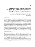
mm in the west to 617 mm in the east. Long term and 2010 mean monthly rainfall, reference
evapotranspiration, and temperature are presented in Fig. 1. Rainfall in 2010 was much
higher than the long term average while evapotranspiration in 2010 was lower than the long
term average.

0
50
100
150
200
250
Jan Feb Mar Apr May Jun Jul Aug Sep Oct Nov Dec
Rain and Evapotranspiration (mm)
Months
Rain 2010 Rain Mean
ETo 2010 ETo Mean
0

5
10
15
20
25
30
Jan Feb Mar Apr May Jun Jul Aug Sep Oct Nov Dec
Tempe rature (
o
C)
Months
2010
Mean
a b

Fig. 1. (a) Rain and reference evapotranspiration ET
o
(long term average and in 2010) (b)
Monthly average temperature (long term average and in 2010) at Wagga Wagga, NSW
(Australia).
A field experiment was carried out during the growing season of 2010 at canola field
experimental site of Wagga Wagga Agricultural Research Institute located at Wagga Wagga
(35
o
03’N; 147
o
21’E; 235 m asl), NSW (Australia). There was enough rainfall (930 mm) in
contrast to long term average of 522 mm in 2010 to provode ideal growing conditions. A
popular variety of canola (Hyola50) was sown on 30 April 2010. The experiment was
conducted on a 24 m x 24 m area. There were 24 plots, 12 experimental plots and 12 buffer

plots. The plots were 6 m long with 1 meter buffer on either end. Plot width was 1.8 m with
a 0.5 m walking strip between plots for data collection.
About a month before the experimental season, neutron probe access tubes were installed to
a depth of 1.5 m for soil moisture measurement. Two access tubes were installed at 2 m from

Evapotranspiration Estimation Using Soil Water Balance, Weather and Crop Data

43
either end of the plot and 2 m from each other. Soil moisture content was measured at 15, 30,
45, 60, 90, and 120 cm depths every two weeks. The probe was calibrated using gravimetric
soil moisture measurements done when access tubes were installed on site.
2.2 Weather data
Daily weather data (rainfall, minimum and maximum temperature, solar radiation, relative
humidity, and wind speed) were collected from the meteorological station of the Wagga
Wagga Agricultural Institute located adjacent to the experimental site. Out of the total
annual rainfall of 930 mm, the amount or proportion (in percentage) during the canola
growing season (May to November) was 514 mm (53%) while the long term average was 333
mm (64% of the long term average of 522 mm). Monthly average maximum and minimum
temperature was 26
o
C and 3
o
C respectively. Reference evapotranspiration ET
o
was
calculated using the procedure described in the FAO Irrigation and Drainage Paper 56
(Allen et al., 1998) with the help of the program FAO ET
o
Calculator (Raes, 2009).
2.3 Soil hydraulic characteristics

A 1.5m x 1.5m x 1.5m soil trench was dug for soil texture, field capacity (θ
FC
), and wilting
point (θ
WP
) determination. Soil samples were retrieved from 0-30, 30-60, 60-90, and 90-120
cm depths for soil texture, θ
FC
, and θ
WP
determination using standard laboratory procedures
hydrometer and pressure plate apparatus apparatus.
2.4 Crop parameters
The following crop phenological stages were recorded during the growing season: planting
date, 90% emergence, beginning and end of flowering, senescence and maturity. The canopy
cover was measured using GreenSeeker
TM
, an Optical Sensor Unit (NTech Industries, Inc.,
USA). GreenSeeker
TM
, is a handheld tool that determines Normalized Difference Vegetative
Index (NDVI), is an integrated optical sensing and application system that measures green
crop canopy cover.
3. Soil water balance method
Rain or irrigation reaching a unit area of soil surface, may infiltrate into the soil, or leave the
area as surface runoff. The infiltrated water may (a) evaporate directly from the soil surface,
(b) taken up by plants for growth or transpiration, (c) drain downward beyond the root zone
as deep percolation, or (d) accumulate within the root zone. The water balance method is
based on the conservation of mass which states that change in soil water content ∆S of a root
zone of a crop is equal to the difference between the amount of water added to the root

zone, Q
i
, and the amount of water withdrawn from it, Q
o
(Hillel, 1998) in a given time
interval expressed as in Eq. (1).

io
SQ Q

 (1)
Eq. (1) can be used to determine evapotranspiration of a given crop as follows
ET P I U R D S

    (2)
where ∆S = change in root zone soil moisture storage, P = Precipitation, I = Irrigation, U =
upward capillary rise into the root zone, R = Runoff, D = Deep percolation beyond the root