Evapotranspiration Remote Sensing and Modeling Part 4 doc
Bạn đang xem bản rút gọn của tài liệu. Xem và tải ngay bản đầy đủ của tài liệu tại đây (1.13 MB, 30 trang )
Hargreaves and Other Reduced-Set Methods for Calculating Evapotranspiration
79
Popova Z, Kercheva M, Pereira LS (2006) Validation of the FAO methodology for computing
ETo with limited data. Application to south Bulgaria. Irrig Drain. 55:201–215.
Rahimikhoob AR (2008) Comparative study of Hargreaves’s and artificial neural network’s
methodologies in estimating reference evapotranspiration in a semiarid
environment. Irrig Sci 26:253–259.
Reis EF, Bragança R, Garcia GO, Pezzopane JEM, Tagliaferre C (2007) Comparative study of
the estimate of evaporate transpiration regarding the three locality state of Espirito
Santo during the dry period. IDESIA (Chile) 25(3) 75-84
Samani Z (2000) Estimating solar radiation and evapotranspiration using minimum
climatological data. J Irrig Drain Engin. 126(4):265–267.
Samani ZA, Pessarakli M (1986) Estimating potential crop evapotranspiration with
minimum data in Arizona. Trans. ASAE (29): 522–524.
Sepaskhah, AR, Razzaghi, FH (2009) Evaluation of the adjusted Thornthwaite and
Hargreaves-Samani methods for estimation of daily evapotranspiration in a semi-
arid region of Iran. Archives of Agronomy and Soil Science, 55: 1, 51- 6
Sentelhas C, Gillespie TJ, Santos EA (2010) Evaluation of FAO Penman–Monteith and
alternative methods for estimating reference evapotranspiration with missing data
in Southern Ontario, Canada. Agricultural Water Management 97: 635–644.
Shahidian, S., Serralheiro, R.P., Teixeira, J.L., Santos, F.L., Oliveira, M.R.G., Costa, J.L.,
Toureiro, C Haie, N. (2007) Desenvolvimento dum sistema de rega automático,
autónomo e adaptativo. I Congreso Ibérico de Agroingeneria.
Shahidian S. , Serralheiro R. , Teixeira J.L., Santos F.L., Oliveira M.R., Costa J., Toureiro C.,
Haie N., Machado R. (2009) Drip Irrigation using a PLC based Adaptive Irrigation
System WSEAS Transactions on Environment and Development, Vol 2- Feb.
Shuttleworth, W.J., and I.R. Calder. (1979) Has the Priestley-Taylor equation any relevance
to the forest evaporation? Journal of Applied Meteorology, 18: 639-646.
Smith, M, R.G. Allen, J.L. Monteith, L.S. Pereira, A. Perrier, and W.O. Pruitt. (1992) Report
on the expert consultation on procedures for revision of FAO guidelines for
prediction of crop water requirements. Land and Water Development Division,
United Nations Food and Agriculture Service, Rome, Italy
Stanhill, G., 1961. A comparison of methods of calculating potential evapotranspiration from
climatic data. Isr. J. Agric. Res.: Bet-Dagan (11), 159–171.
Teixeira JL, Shahidian S, Rolim J (2008) Regional analysis and calibration for the South of
Portugal of a simple evapotranspiration model for use in an autonomous landscape
irrigation controller.
Thornthwaite CW (1948) An approach toward a rational classification of climate. Geograph
Rev.38:55–94.
Trajkovic S. (2005) Temperature-based approaches for estimating reference
evapotranspiration. J Irrig Drain Engineer. 131(4):316–323
Trajkovic S (2007) Hargreaves versus Penman-Monteith under Humid Conditions Journal of
Irrigation and Drainage Engineering, Vol. 133, No. 1, February 1.
Trajkovic, S, Stojnic, V. (2007) Effect of wind speed on accuracy of Turc Method in a humid
climate. Facta Universitatis. 5(2):107-113
Evapotranspiration – Remote Sensing and Modeling
80
Xu, CY, Singh, VP (2000) Evaluation and Generalization of Radiation-based Methods for
Calculating Evaporation, Hydrolog. Processes 14: 339–349.
Xu CY, Singh VP (2002) Cross Comparison of Empirical Equations for Calculating Potential
evapotranspiration with data from Switzerland. Water Resources Management 16:
197-219.
5
Fuzzy-Probabilistic Calculations of
Evapotranspiration
Boris Faybishenko
Lawrence Berkeley National Laboratory
Berkeley, CA
USA
1. Introduction
Evaluation of evapotranspiration uncertainty is needed for proper decision-making in the
fields of water resources and climatic predictions (Buttafuoco et al., 2010; Or and Hanks,
1992; Zhu et al., 2007). However, in spite of the recent progress in soil-water and climatic
uncertainty quantification, using stochastic simulations, the estimates of potential
(reference) evapotranspiration (E
o
) and actual evapotranspiration (ET) using different
methods/models, with input parameters presented as PDFs or fuzzy numbers, is a
somewhat overlooked aspect of water-balance uncertainty evaluation (Kingston et al., 2009).
One of the reasons for using a combination of different methods/models and presenting the
final results as fuzzy numbers is that the selection of the model is often based on vague,
inconsistent, incomplete, or subjective information. Such information would be insufficient
for constructing a single reliable model with probability distributions, which, in turn, would
limit the application of conventional stochastic methods.
Several alternative approaches for modeling complex systems with uncertain models and
parameters have been developed over the past ~50 years, based on fuzzy set theory and
possibility theory (Zadeh, 1978; 1986; Dubois & Prade, 1994; Yager & Kelman, 1996). Some of
these approaches include the blending of fuzzy-interval analysis with probabilistic methods
(Ferson & Ginzburg, 1995; Ferson, 2002; Ferson et al., 2003). This type of analysis has
recently been applied to hydrological research, risk assessment, and sustainable water-
resource management under uncertainty (Chang, 2005), as well as to calculations of E
o
, ET,
and infiltration (Faybishenko, 2010).
The objectives of this chapter are to illustrate the application of a combination of probability
and possibility conceptual-mathematical approaches—using fuzzy-probabilistic models—
for predictions of potential evapotranspiration (E
o
) and actual evapotranspiration (ET) and
their uncertainties, and to compare the results of calculations with field evapotranspiration
measurements.
As a case study, statistics based on monthly and annual climatic data from the Hanford site,
Washington, USA, are used as input parameters into calculations of potential
evapotranspiration, using the Bair-Robertson, Blaney-Criddle, Caprio, Hargreaves, Hamon,
Jensen-Haise, Linacre, Makkink, Penman, Penman-Monteith, Priestly-Taylor, Thornthwaite,
and Turc equations. These results are then used for calculations of evapotranspiration based
on the modified Budyko (1974) model. Probabilistic calculations are performed using Monte
Evapotranspiration – Remote Sensing and Modeling
82
Carlo and p-box approaches, and fuzzy-probabilistic and fuzzy simulations are conducted
using the RAMAS Risk Calc code. Note that this work is a further extension of this author’s
recently published work (Faybishenko, 2007, 2010).
The structure of this chapter is as follows: Section 2 includes a review of semi-empirical
equations describing potential evapotranspiration, and a modified Budyko’s model for
evaluating evapotranspiration. Section 3 includes a discussion of two types of
uncertainties—epistemic and aleatory uncertainties—involved in assessing
evapotranspiration, and a general approach to fuzzy-probabilistic simulations by means of
combining possibility and probability approaches. Section 4 presents a summary of input
parameters and the results of E
o
and ET calculations for the Hanford site, and Section 5
provides conclusions.
2. Calculating potential evapotranspiration and evapotranspiration
2.1 Equations for calculations of potential evapotranspiration
The potential (reference) evapotranspiration E
o
is defined as evapotranspiration from a
hypothetical 12 cm grass reference crop under well-watered conditions, with a fixed surface
resistance of 70 s m
-1
and an albedo of 0.23 (Allen et al., 1998). Note that this subsection
includes a general description of equations used for calculations of potential
evapotranspiration; it does not provide an analysis of the various advantages and
disadvantages in applying these equations, which are given in other publications (for
example, Allen et al., 1998; Allen & Pruitt, 1986; Batchelor, 1984; Maulé et al., 2006; Sumner
& Jacobs, 2005; Walter et al., 2002).
The two forms of Baier-Robertson equations (Baier, 1971; Baier & Robertson, 1965) are given
by:
E
o
= 0.157T
max
+ 0.158 (T
max
- T
min
) + 0.109R
a
- 5.39 (1)
E
o
= -0.0039T
max
+ 0.1844(T
max
- T
min
) + 0.1136 R
a
+ 2.811(e
s
− e
a
) − 4.0 (2)
where E
o
= daily evapotranspiration (mm day
-1
); T
max
= the maximum daily air temperature,
o
C; T
min
= minimum temperature,
o
C; R
a
= extraterrestrial radiation (MJ m
-2
day
-1
) (ASCE
2005), e
s
= saturation vapor pressure (kPa), and e
a
= mean actual vapor pressure (kPa).
Equation (1) takes into account the effect of temperature, and Equation (2) takes into account
the effects of temperature and relative humidity.
The Blaney-Criddle equation (Allen & Pruitt, 1986) is used to calculate evapotranspiration
for a reference crop, which is assumed to be actively growing green grass of 8–15 cm height:
E
o
= p (0.46·T
mean
+ 8) (3)
where E
o
is the reference (monthly averaged) evapotranspiration (mm day
−1
), T
mean
is the
mean daily temperature (°C) given as T
mean
= (T
max
+ T
min
)/2, and p is the mean daily
percentage of annual daytime hours.
The Caprio (1974) equation for calculating the potential evapotranspiration is given by
E
o
= 6.1·10
-6
R
s
[(1.8 ·T
mean
) + 1.0] (4)
where E
o
= mean daily potential evapotranspiration (mm day
-1
); R
s
= daily global (total)
solar radiation (kJ m
-2
day
-1
); and T
mean
= mean daily air temperature (°C).
Fuzzy-Probabilistic Calculations of Evapotranspiration
83
The Hansen (1984) equation is given by:
E
o
= 0.7 / ( + ) · R
i
/ (5)
where = slope of the saturation vapor pressure vs. temperature curve, = psychrometric
constant, R
i
= global radiation, and = latent heat of water vaporization.
The Hargreaves equation (Hargreaves & Samani, 1985) is given by
E
o
= 0.0023(T
mean
+ 17.8)(T
max
- T
min
)
0.5
R
a
(6)
where both E
o
and R
a
(extraterrestrial radiation) are in millimeters per day
-1
(mm day
-1
).
The Jensen and Haise (1963) equation is given by
E
o
= R
s
/2450 [(0.025 T
mean
) + 0.08] (7)
where E
o
= monthly mean of daily potential evapotranspiration (mm day
-1
); R
s
= monthly
mean of daily global (total) solar radiation (kJ m
-2
day
-1
); and T
mean
= monthly mean
temperature.
The Linacre (1977) equation is given by:
E
o
= [500T
m
/ (100-L) + 15(T-Td)] / (80-T) (8)
where E
o
is in mm day
-1
, T
m
= temperature adjusted for elevation, T
m
= T + 0.006h (°C), h =
elevation (m), T
d
= dew point temperature (°C), and L = latitude (°).
The Makkink (1957) model is given by
E
o
= 0.61 / ( + ) R
s
/2.45 – 0.12 (9)
where R
s
= solar radiation (MJ m
-2
day
-1
), and and are the parameters defined above.
The Penman (1963) equation is given by
E
o
= mR
n
+ 6.43(1+0.536 u
2
) e /
v
(m + ) (10)
where
= slope of the saturation vapor pressure curve (kPa K
-1
), R
n
= net irradiance (MJ m
-2
day
-1
), ρ
a
= density of air (kg m
-3
), c
p
= heat capacity of air (J kg
-1
K
-1
), e = vapor pressure
deficit (Pa),
v
= latent heat of vaporization (J kg
-1
),
= psychrometric constant (Pa K
-1
), and
E
o
is in units of kg/(m²s).
The general form of the Penman-Monteith equation (Allen et al., 1998) is given by
E
o
= [0.408 (R
n
– G) + C
n
/(T+273) u
2
(e
s
-e
a
)] / [ + (1+C
d
u
2
)] (11)
where E
o
is the standardized reference crop evapotranspiration (in mm day
-1
) for a short
(0.12 m, with values C
n
=900 and C
d
=0.34) reference crop or a tall (0.5 m, with values C
n
=1600
and C
d
=0.38) reference crop, R
n
= net radiation at the crop surface (MJ m
-2
day
-1
), G = soil
heat flux density (MJ m
-2
day
-1
), T = air temperature at 2 m height (°C), u
2
= wind speed at 2
m height (m s
-1
), e
s
= saturation vapor pressure (kPa), e
a
= actual vapor pressure (kPa), (e
s
-
e
a
) = saturation vapor pressure deficit (kPa), = slope of the vapor pressure curve (kPa °C
-1
),
and = psychrometric constant (kPa °C
-1
).
The Priestley–Taylor (1972) equation is given by
E
o
= 1/ (R
n
– G) / () (12)
Evapotranspiration – Remote Sensing and Modeling
84
where = latent heat of vaporization (MJ kg
-1
), R
n
= net radiation (MJ m
-2
day
-1
), G = soil
heat flux (MJ m
-2
day
-1
), = slope of the saturation vapor pressure-temperature relationship
(kPa °C
-1
), = psychrometric constant (kPa °C
-1
), and = 1.26. Eichinger et al. (1996) showed
that is practically constant for all typically observed atmospheric conditions and
relatively insensitive to small changes in atmospheric parameters. (On the other hand,
Sumner and Jacobs [2005] showed that is a function of the green-leaf area index [LAI] and
solar radiation.)
The Thornthwaite (1948) equation is given by
E
o
= 1.6 (L/12) (N/30) (10 T
mean (i)
/I)
(13)
where E
o
is the estimated potential evapotranspiration (cm/month), T
mean (i)
= average
monthly (i) temperature (
o
C); if T
mean (i)
< 0, Eo = 0 of the month (i) being calculated, N =
number of days in the month, L = average day length (hours) of the month being calculated,
and I = heat index given by
1.514
12
mean( )
1
5
i
i
T
I
and = (6.75·10
-7
) I
3
– (7.71·10
-5
) I
2
+ (1.792·10
-2
)I + 0.49239
The Turc (1963) equation is given by
E
o
= (0.0239 · R
s
+ 50) [0.4/30 · T
mean
/ (T
mean
+ 15.0)] (14)
where E
o
= mean daily potential evapotranspiration (mm/day); R
s
= daily global (total) solar
radiation (kJ/m
2
/day); T
mean
= mean daily air temperature (°C).
2.2 Modified Budyko’s equation for evaluating evapotranspiration
For regional-scale, long-term water-balance calculations within arid and semi-arid areas, we
can reasonably assume that (1) soil water storage does not change, (2) lateral water motion
within the shallow subsurface is negligible, (3) the surface-water runoff and runon for
regional-scale calculations simply cancel each other out, and (4) ET is determined as a
function of the aridity index, ET=f(where E
o
/P, which is the ratio of potential
evapotranspiration, E
o
, to precipitation, P (Arora 2002).
Budyko’s (1974) empirical formula for the relationship between the ratio of ET/P and the
aridity index was developed using the data from a number of catchments around the world,
and is given by:
ET/P = { tanh (1/exp (-)]}
0.5
(15)
Equation (1) can also be given as a simple exponential expression (Faybishenko, 2010):
ET/P=a[1-exp(-b
)] (16)
with coefficients a =0.9946 and b =1.1493. The correlation coefficient between the calculations
using (15) and (16) is R=0.999. Application of the modified Budyko’s equation, given by an
exponential function (2) with the
value in single term, will simplify further calculations of
ET.
Fuzzy-Probabilistic Calculations of Evapotranspiration
85
3. Types of uncertainties in calculating evapotranspiration and simulation
approaches
3.1 Epistemic and aleatory uncertainties
The uncertainties involved in predictions of evapotranspiration, as a component of soil-
water balance, can generally be categorized into two groups—aleatory and epistemic
uncertainties. Aleatory uncertainty arises because of the natural, inherent variability of soil
and meteorological parameters, caused by the subsurface heterogeneity and variability of
meteorological parameters. If sufficient information is available, probability density
functions (PDFs) of input parameters can be used for stochastic simulations to assess
aleatory evapotranspiration uncertainty. In the event of a lack of reliable experimental data,
fuzzy numbers can be used for fuzzy or fuzzy-probabilistic calculations of the aleatory
evapotranspiration uncertainty (Faybishenko 2010).
Epistemic uncertainty arises because of a lack of knowledge or poor understanding,
ambiguous, conflicting, or insufficient experimental data needed to characterize coupled-
physics phenomena and processes, as well as to select or derive appropriate conceptual-
mathematical models and their parameters. This type of uncertainty is also referred to as
subjective or reducible uncertainty, because it can be reduced as new information becomes
available, and by using various models for uncertainty evaluation. Generally, variability,
imprecise measurements, and errors are distinct features of uncertainty; however, they are
very difficult, if not impossible, to distinguish (Ferson & Ginzburg, 1995).
In this chapter the author will consider the effect of aleatory uncertainty on
evapotranspiration calculations by assigning the probability distributions of input
meteorological parameters, and the effect of epistemic uncertainty is considered by using
different evapotranspiration models.
3.2 Simulation approaches
3.2.1 Probability approach
A common approach for assessing uncertainty is based on Monte Carlo simulations, using
PDFs describing model parameters. Another probability-based approach to the specification
of uncertain parameters is based on the application of probability boxes (Ferson, 2002;
Ferson et al., 2003). The probability box (p-box) approach is used to impose bounds on a
cumulative distribution function (CDF), expressing different sources of uncertainty. This
method provides an envelope of distribution functions that bounds all possible
dependencies. An uncertain variable x expressed with a probability distribution, as shown
in Figure 1a, can be represented as a variable that is bounded by a p-box [
F , F ], with the
right curve
F (x) bounding the higher values of x and the lower probability of x, and the left
curve F (x) bounding the lower values and the higher probability of x. With better or
sufficiently abundant empirical information, the p-box bounds are usually narrower, and
the results of predictions come close to a PDF from traditional probability theory.
3.2.2 Possibility approach
In the event of imprecise, vague, inconsistent, incomplete, or subjective information about
models and input parameters, the uncertainty is captured using
fuzzy modeling theory, or
possibility theory, introduced by Zadeh (1978). For the past 50 years or so, possibility theory
has successfully been applied to describe such systems as complex, large-scale engineering
systems, social and economic systems, management systems, medical diagnostic processes,
human perception, and others. The term
fuzziness is, in general, used in possibility theory to
Evapotranspiration – Remote Sensing and Modeling
86
0
0.1
0.2
0.3
0.4
0.5
0.6
0.7
0.8
0.9
1
6 8 10 12 14 16
x
FMF/Possibility
(b)
Fig. 1. Graphical illustration of uncertain numbers: (a) Cumulative normal distribution
function (dashed line), with mean=10 and standard deviation =1, and a p-box—left bound
with mean=9.5 and =0.9, and right bound with mean=10.5 and =1.1; and (b) Fuzzy
trapezoidal (solid line) number, plotted using Eq. (17) with a=6, b=9, c=11, and d=14.
Interval [b,c]=[9, 11] corresponds to FMF=1. Triangular (short dashes) and Gaussian (long
dashes) fuzzy numbers are also shown. Figure (b) also shows an -cut=0.5 (thick horizontal
line) through the trapezoidal fuzzy number (Faybishenko 2010).
describe objects or processes that cannot be given precise definition or precisely measured.
Fuzziness identifies a class (set) of objects with nonsharp (i.e., fuzzy) boundaries, which may
result from imprecision in the meaning of a concept, model, or measurements used to
characterize and model the system. Fuzzification implies replacing a set of crisp (i.e.,
precise) numbers with a set of fuzzy numbers, using fuzzy membership functions based on
the results of measurements and perception-based information (Zadeh 1978). A fuzzy
number is a quantity whose value is imprecise, rather than exact (as is the case of a single-
valued number). Any fuzzy number can be thought of as a function whose domain is a
specified set of real numbers. Each numerical value in the domain is assigned a specific
“grade of membership,” with 0 representing the smallest possible grade (full
nonmembership), and 1 representing the largest possible grade (full membership). The
grade of membership is also called the degree of possibility and is expressed using fuzzy
membership functions (FMFs). In other words, a fuzzy number is a fuzzy subset of the
domain of real numbers, which is an alternative approach to expressing uncertainty.
Several types of FMFs are commonly used to define fuzzy numbers: triangular, trapezoidal,
Gaussian, sigmoid, bell-curve, Pi-,
S-, and Z-shaped curves. As an illustration, Figure 1b
shows a trapezoidal fuzzy number given by
0,
,
() 1,
,
0,
xa
xa
axb
ba
fx b x c
dx
cxd
dc
dx
, (17)
Fuzzy-Probabilistic Calculations of Evapotranspiration
87
where coefficients a, b, c , and d are used to define the shape of the trapezoidal FMF. When
a= b, the trapezoidal number becomes a triangular fuzzy number.
Figure 1b also illustrates one of the most important attributes of fuzzy numbers, which is the
notion of an -cut. The -cut interval is a crisp interval, limited by a pair of real numbers.
An -cut of 0 of the fuzzy variable represents the widest range of uncertainty of the variable,
and an -cut value of 1 represents the narrowest range of uncertainty of the variable.
Possibility theory is generally applicable for evaluating all kinds of uncertainty, regardless
of its source or nature. It is based on the application of both hard data and the subjective
(perception-based) interpretation of data. Fuzzy approaches provide a distribution
characterizing the results of all possible magnitudes, rather than just specifying upper or
lower bounds. Fuzzy methods can be combined with calculations of PDFs, interval
numbers, or p-boxes, using the RAMAS Risk Calc code (Ferson 2002). In this paper, the
RAMAS Risk Calc code is used to assess the following characteristic parameters of the fuzzy
numbers and p-boxes:
Mean—an interval between the means of the lower (left) and upper (right) bounds of
the uncertain number x.
Core—the most possible value(s) of the uncertain number x, i.e., value(s) with a
possibility of one, or for which the probability can be any value between zero and one.
Iqrange—an interval guaranteed to enclose the interquartile range (with endpoints at
the 25th and 75th percentiles) of the underlying distribution.
Breadth of uncertainty—for fuzzy numbers, given by the area under the membership
function; for p-boxes, given by the area between the upper and lower bounds. The
uncertainty decreases as the breadth of uncertainty decreases.
When fuzzy measures serve as upper bounds on probability measures, one could expect to
obtain a conservative (bounding) prediction of system behavior. Therefore, fuzzy
calculations may overestimate uncertainty. For example, the application of fuzzy methods is
not optimal (i.e., it overestimates uncertainty) when sufficient data are available to construct
reliable PDFs needed to perform a Monte Carlo analysis.
In a recent paper (Faybishenko 2010), this author demonstrated the application of the fuzzy-
probabilistic method using a hybrid approach, with direct calculations, when some
quantities can be represented by fuzzy numbers and other quantities by probability
distributions and interval numbers (Kaufmann and Gupta 1985; Ferson 2002; Guyonnet et
al. 2003; Cooper et al. 2006). In this paper, the author combines (aggregates) the results of
Monte Carlo calculations with multiple E
o
models by means of fuzzy numbers and p-boxes,
using the RAMAS Risk Calc software (Ferson 2002).
4. Hanford case study
4.1 Input parameters and modeling scenarios for the Hanford Site
The Hanford Site in Southeastern Washington State is one of the largest environmental
cleanup sites in the USA, comprising 1,450 km
2
of semiarid desert. Located north of
Richland, Washington, the Hanford Site is bordered on the east by the Columbia River and
on the south by the Yakima River, which joins the Columbia River near Richland, in the
Pasco Basin, one of the structural and topographic basins of the Columbia Plateau. The areal
topography is gently rolling and covered with unconsolidated materials, which are
sufficiently thick to mask the surface irregularities of the underlying material. Areas
adjacent to the Hanford Site are primarily agricultural lands.
Evapotranspiration – Remote Sensing and Modeling
88
Meteorological parameters used to assign model input parameters were taken from the
Hanford Meteorological Station (HMS—see located at the center of
the Hanford Site just outside the northeast corner of the 200 West Area, as well as from
publications (DOE, 1996; Hoitink et al., 2002; Neitzel, 1996.) At the Hanford Site, the E
o
is
estimated to be from 1,400 to 1,611 mm/yr (Ward et al. 2005), and the ET is estimated to be
160 mm/yr (Figure 2). A comparison of field estimates with the results of calculations
performed in this paper is shown in Section 4.2. Calculations are performed using the
temperature and precipitation time-series data representing a period of active soil-water
balance (i.e., with no freezing) from March through October for the years 1990–2007. A set of
meteorological parameters is summarized in Table 1, which are then used to develop the
input PDFs and fuzzy numbers shown in Figure 3.
Several modeling scenarios were developed (Table 2) to assess how the application of
different models for input parameters affects the uncertainty of E
o
and ET calculations. For
the sake of simulation simplicity, the input parameters are assumed to be independent
variables. Scenarios 0 to 8, described in detail in Faybishenko (2010), are based on the
application of a single Penman model for E
o
calculations, with annual average values of
input parameters. Scenario 0 was modeled using input PDFs by means of Monte Carlo
simulations, using RiskAMP Monte Carlo Add-In Library version 2.10 for Excel. Scenarios 1
through 8 were simulated by means of the RAMAS Risk Calc code. Scenario 1 was
simulated using input PDFs, and the results are given as p-box numbers. Scenarios 2
through 6 were simulated applying both PDFs and fuzzy number inputs, corresponding to
-cuts from 0 to 1). Scenarios 7 and 8 were simulated using only fuzzy numbers. The
calculation results of Scenarios 0 through 8 are compared in this chapter with newly
calculated Scenarios 9 and 10, which are based on Monte Carlo calculations by means of all
E
o
models, described in Section 2, and then bounding the resulting PDFs by a trapezoidal
fuzzy number (Scenario 9) and the p-box (Scenario 10).
Type
of data
Parameters Wind
speed
(km/hr)
Relative
humidity
(%)
Albedo Solar
radiation
(Ly/day)
Annual
precipi-
tation
(mm/yr)
Temperature
(
o
C)
Max Min Max Min
PDFs Mean
15.07 80.2 33.3 0.21 332.55 185 33.41 2.87
Standard
Deviation
0.92 4.01 1.66 0.021 16.63 55.62 1.08 1.11
Trape-
zoidal
FMFs
= 0
Min
12.31 68.17 28.29 0.15 282.66 46.0 30.17 0.0
Max
17.84 92.23 38.31 0.27 382.44 324.1 36.65 6.17
=1
Min
14.61 78.2 32.47 0.22 324.24 157.2 32.87 2.32
Max
15.53 82.2 34.14 0.27 382.44 212.8 33.95 3.42
Table 1. Meteorological parameters from the Hanford Meteorological Station used for E
o
calculations for all scenarios (the data sources are given in the text).
Fuzzy-Probabilistic Calculations of Evapotranspiration
89
Fig. 2. Estimated water balance ET and recharge/infiltration at the Hanford site (Gee et al,
2007).
Scenarios
Input parameters Output
para-
meters
W
ind
speed
Humidity Albedo Solar
radiation
Precipi
-
tation
Tempe-
rature
0 PDF PDF PDF PDF PDF PDF PDF
1 PDF PDF PDF PDF PDF PDF
p
-box
2 Fuzz
y
PDF PDF PDF PDF PDF H
y
brid
3 Fuzz
y
Fuzz
y
PDF PDF PDF PDF H
y
brid
4 Fuzz
y
Fuzz
y
Fuzz
y
PDF PDF PDF H
y
brid
5 Fuzz
y
Fuzz
y
Fuzz
y
Fuzz
y
PDF PDF H
y
brid
6 Fuzz
y
Fuzz
y
Fuzz
y
Fuzz
y
Fuzz
y
PDF H
y
brid
7
1)
Fuzz
y
Fuzz
y
Fuzz
y
Fuzz
y
Fuzz
y
Fuzz
y
Fuzz
y
8
2)
Fuzz
y
Fuzz
y
Fuzz
y
Fuzz
y
Fuzz
y
Fuzz
y
Fuzz
y
9
3)
PDF PDF PDF PDF PDF PDF Fuzz
y
10
3)
PDF PDF PDF PDF PDF PDF
p
-box
Notes:
1)
In Scenario 7, all FMFs are trapezoidal.
2)
In Scenario 8, all FMFs are triangular: the mean values of parameters, which are given in Table 1, are
used for =1; and the minimum and maximum values of parameters, given in Table 1 for trapezoidal
FMFs (Scenario 7), are also used for =0 of triangular FMFs in Scenario 8.
3)
In Scenarios 9 and 10, input parameters are monthly averaged.
Table 2. Scenarios of input and output parameters used for water-balance calculations
(Scenarios 0, and 1-8 are from Faybishenko, 2010).
Evapotranspiration – Remote Sensing and Modeling
90
4.2 Results and comparison with field data
4.2.1 Potential evapotranspiration (E
o
)
Figure 4a shows cumulative distributions of E
o
from different models, along with an
aggregated p-box, and Figure 4b shows the corresponding FMFs (calculated as normalized
PDFs) of E
o
from different models, along with an aggregated trapezoidal fuzzy E
o
. These
figures illustrate that the Baier-Robertson (Eq. 1), Blaney-Criddle (Eq. 3), Hargreaves (Eq. 6),
Penman (Eq. 10), Penman-Monteith (Eq. 11) (for tall plants), and Priestly-Taylor (Eq. 12)
models provide the best match with field data, while the Makkink (Eq. 9) and Thornthwaite
(Eq. 13) models significantly underestimate the E
o
, and the Linacre (Eq. 8) and Baier-
Robertson (Eq. 2) models greatly overestimate E
o
.
0
0.2
0.4
0.6
0.8
1
0 100 200 300 400
Precipitatin (mm/day)
Probability/FMF
0
0.2
0.4
0.6
0.8
1
20 40 60 80 100
Humidity (%)
Probability/FMF
min
max
0
0.2
0.4
0.6
0.8
1
010203040
Temperature (oC)
Probability/FMF
min
max
0
0.2
0.4
0.6
0.8
1
0.1 0.15 0.2 0.25 0.3
A
lbedo
Probability /FM F
0
0.2
0.4
0.6
0.8
1
10 12 14 16 18 20
Wind (km/d)
Probability/FMF
0
0.2
0.4
0.6
0.8
1
250 300 350 400
Solar radiation (Ly/d)
Probability/FMF
Fig. 3. Input PDFs (solid lines) and fuzzy numbers (dashed lines) used for calculations
(Faybishenko, 2010).
Fuzzy-Probabilistic Calculations of Evapotranspiration
91
Figure 5a demonstrates that the E
o
mean from Monte Carlo simulations is within the mean
ranges from the p-box (Scenario 1) and fuzzy-probabilistic scenarios (Scenarios 2-6). It also
corresponds to a midcore of the fuzzy scenario with trapezoidal FMFs (Scenario 7), the core
of the fuzzy scenario with triangular FMFs (Scenario 8), and the centroid values of the fuzzy
E
o
of Scenario 9, as well as a p-box of Scenario 10.
Fig. 4. (a) Cumulative probability of potential evapotranspiration calculated using different
E
o
formulae; an aggregated p-box, which is shown by a black line with solid squares: normal
distribution with the left/minimum curve—mean=933, var=1070, and the right /max
curve—mean=1763, var=35755; and (b) corresponding fuzzy numbers (calculated from
normalized PDFs); an aggregated trapezoidal fuzzy number is shown by a black line—Eq.
(17) with a=772, b=933, c=1763, and d=2222. (all numbers of E
o
are in mm/yr)
The range of means from the p-box and fuzzy-probabilistic calculations for =1 is practically
the same, indicating that including fuzziness within the input parameters does not change
the range of most possible E
o
values. Figure 5a shows that the core uncertainty of the
trapezoidal FMFs (Scenario 7) is the same as the uncertainty of means for fuzzy-probabilistic
calculations for =1. Obviously, the output uncertainty decreases for the input triangular
FMFs (Scenario 8), because these FMFs resemble more tightly the PDFs used in other
scenarios. Figure 5a also illustrates that a relatively narrow range of field estimates of E
o
—
from 1,400 to 1,611 mm/yr for the Hanford site (Ward 2005)—is well within the calculated
uncertainty of E
o
values. Note from Figure 5a that the uncertainty ranges from p-box,
hybrid, and fuzzy calculations significantly exceed those from Monte Carlo simulations for a
single Penman model, but are practically the same as those from calculations using multiple
E
o
models.
Characteristic parameters (Figures 5a) and the breadth of uncertainty (Figure 6a) of E
o
calculated from multiple models—Scenarios 9 and 10—are in a good agreement with field
measurements and other calculation scenarios.
4.2.2 Evapotranspiration (ET)
Figure 5b shows that the mean ET of ~184 mm/yr from Monte Carlo simulations
(Scenario 0) is practically the same as the ET means for Scenarios 1 through 5 and the core
value for Scenario 8. The greater ET uncertainty for Scenario 6 (precipitation is simulated
using a fuzzy number) can be explained by the relatively large precipitation range for
=0—from 46 to 324 mm/yr. At the same time, the means of ET values for =1 range
Evapotranspiration – Remote Sensing and Modeling
92
within relatively narrow limits, as the precipitation for =1 changes from 157.2 to 212.8
mm/yr (see Table 1).
The breadth of uncertainty of ET (Figure 6b) is practically the same for Scenarios 1 through
5, increase for Scenarios 6, 7, and 8 in the account of calculations using a fuzzy precipitation,
and then decrease for Scenarios 9 and 10 using multiple E
o
models. A smaller range of ET
uncertainty calculated using multiple E
o
models can be explained by the fact that the
Budyko curve asymptotically reaches the limit of ET/P=1 for high values of the aridity
index, which are typical for the semi-arid climatic conditions of the Hanford site.
1543
1241
1235
1549
1229
1557
1215
1576
1215
1576
1458
1447
1423
1369
400
800
1200
1600
2000
2400
012345678910
Scenario
E o (mm.yr)
Fuzzy-probabilistic Fuzzy
p-boxMC
(a)
Field
Fuzzy-
Prob
p-box
Penman model
Multiple
models
184184
322.4
156.1
211.7
184
163
163
163.2
184.5
180.1
184.6
180
184.6
179.8
184.6
179.4
43.1
185.2
179.4
163.2
40
90
140
190
240
290
340
012345678910
Scenario
ET (mm/yr)
(b)
Field
Fig. 5. Results of calculations of E
o
(a) and ET (b) and comparison with field measurements.
Red vertical lines are the mean intervals (Scenarios 1-6, and 10) and core intervals (Scenarios
7, 8, and 9), the blue diamonds indicate the interquartile ranges with endpoints at the 25
th
and 75
th
percentiles of the underlying distribution. Red open diamonds for Scenarios 2-6
indicate the mean intervals for the hybrid level=10 (Faybishenko 2010), and red solid
diamonds for Scenarios 7-10 indicate centroid values. The height of a shaded area in figure a
indicates the range of E
o
from field measurements. (Results of calculations of Scenarios 0-8
are from Faybishenko, 2010.)
Fuzzy-Probabilistic Calculations of Evapotranspiration
93
The calculated means for Scenarios 0, 1–5, and 8 exceed the field estimates of ET of 160
mm/yr (Gee et al., 1992; 2007) by 22 to 24 mm/yr. This difference can be explained by Gee
et al. using a lower value of annual precipitation (160 mm/yr for the period prior to 1990) in
their calculations, while our calculations are based on using a greater mean annual
precipitation (185 mm/yr), averaged for the years from 1990 to 2007. The field-based data
are within the ET uncertainty range for Scenarios 6 and 7, since the precipitation range is
wider for these scenarios. Calculations using multiple E
o
models generated the ET values
(Scenarios 9 and 10), which are practically the same as those from field measurements.
600
800
1000
1200
1400
12345678910
Scenario
E o breadth (mm/yr)
(a)
Fuzzy-probabilistic Fuzzy
p-boxMC
Fuzzy-
Prob
p-box
Penman model
Multiple
models
1
10
100
1000
12345678910
Scenario
ET breadth (mm/yr)
(b)
Fig. 6. Breadth of uncertainty of E
o
and ET. For Scenarios 2-6, grey and white bars indicate
the maximum and minimum uncertainty, correspondingly. (Results of calculations of
Scenarios 0-8 are from Faybishenko, 2010.)
5. Conclusions
The objectives of this chapter are to illustrate the application of a fuzzy-probabilistic
approach for predictions of E
o
and ET, and to compare the results of calculations with those
Evapotranspiration – Remote Sensing and Modeling
94
from field measurements at the Hanford site. Using historical monthly averaged data from
the Hanford Meteorological Station, this author employed Monte-Carlo simulations to
assess the frequency distribution and statistics of input parameters for these models, which
are then used as input into probabilistic simulations. The effect of aleatory uncertainty on
calculations of evapotranspiration is assessed by assigning the probability distributions of
input meteorological parameters, and the combined effect of aleatory and epistemic (model)
uncertainty is then expressed by means of aggregating the results of calculations using a p-
box and fuzzy numbers. To illustrate the application of these approaches, the potential
evapotranspiration is calculated using the Bair-Robertson, Blaney-Criddle, Caprio,
Hargreaves-Samani, Hamon, Jensen-Haise, Linacre, Makkink, Priestly-Taylor, Penman,
Penman-Monteith, Thornthwaite, and Turc models, and evapotranspiration is then
determined based on the modified Budyko (1974) model. Probabilistic and fuzzy-
probabilistic calculations using multiple E
o
models generate the E
o
and ET results, which are
well within the range of field measurements and the application of a single Penman model.
The Baier-Robertson, Blaney-Criddle, Hargreaves, Penman, Penman-Monteith, and Priestly-
Taylor models provide the best match with field data.
6. Acknowledgment
This work was partially supported by the Director, Office of Science, Office of Biological and
Environmental Remediation Sciences of the U.S. Department of Energy, and the DOE EM-32
Office of Soil and Groundwater Remediation (ASCEM project) under Contract No. DE-
AC02-05CH11231 to Lawrence Berkeley National Laboratory.
7. References
Allen, R.G. & Pruitt, W.O. (1986), Rational Use of the FAO Blaney-Criddle Formula, Journal
of Irrigation and Drainage Engineering, Vol. 112, No. 2, pp. 139-155,
doi 10.1061/(ASCE)0733-9437(1986)112:2(139)
Allen, R.G.; Pereira L.S.; Raes, D. & Smith, M. (1998). Crop evapotranspiration - Guidelines
for computing crop water requirements - FAO Irrigation and drainage paper 56.
Arora V.K. (2002). The use of the aridity index to assess climate change effect on annual
runoff, J. of Hydrology, Vol. 265, pp. 164–177.
ASCE (2005). The ASCE Standardized Reference Evapotranspiration Equation. Edited by R.
G. Allen, I.A. Walter, R.; Elliott, T. Howell, D. Itenfisu, and M. Jensen. New York,
NY: American Society of Civil Engineers.
Baier, W. & Robertson, G.W. 1965. Estimation of latent evaporation from simple weather
observations. Can. J. Soil Sci. 45, pp. 276-284.
Baier, W. (1971). Evaluation of latent evaporation estimates and their conversion to potential
evaporation. Can. J. of Plant Sciences 51, pp. 255-266.
Budyko, M.I. (1974).Climate and Life, Academic, San Diego, Calif., 508 pp.
Buttafuoco, G.; Caloiero, T.; & Coscarelli, R. (2010). Spatial uncertainty assessment in
modelling reference evapotranspiration at regional scale, Hydrol. Earth Syst. Sci., 14,
pp. 2319-2327, doi:10.5194/hess-14-2319-2010, 2010.
Fuzzy-Probabilistic Calculations of Evapotranspiration
95
Caprio, J.M. (1974). The Solar Thermal Unit Concept in Problems Related to Plant
Development and Potential Evapotranspiration. In: H. Lieth (Editor), Phenology and
Seasonality Modeling. Ecological Studies. Springer Verlag, New York, pp. 353-364.
Chang N-B (2005). Sustainable water resources management under uncertainty, Stochast
Environ Res and Risk Assess, 19, pp. 97–98.
Cooper J.A.; Ferson, S.; & Ginzburg, L. (2006). Hybrid processing of stochastic and subjective
uncertainty data, Risk Analysis, Vol. 16, No. 6, pp. 785–791.
DOE (1996). Final Environmental Impact Statement for the Tank Waste Remediation System,
Hanford Site, Richland, Washington, DOE/EIS-0189. Available from
Dubois, D. & Prade, H. (1994). Possibility theory and data fusion in poorly informed
environments. Control Engineering Practice 2(5), pp. 811-823.
Eichinger W.E.; Parlange, M.B. & Stricker H. (1996). On the Concept of Equilibrium
Evaporation and the Value of the Priestley-Taylor Coefficient, Water Resour. Res.,
32(1): 161-164, doi:10.1029/95WR02920.
Faybishenko, B. (2007). Climatic Forecasting of Net Infiltration at Yucca Mountain Using
Analogue Meteorological Data, Vadose Zone Journal, 6: 77–92.
Faybishenko, B. (2010), Fuzzy-probabilistic calculations of water-balance uncertainty,
Stochastic Environmental Research and Risk Assessment, Vol. 24, No. 6, pp. 939–952.
Ferson, S. (2002). RAMAS Risk Calc 4.0 Software: Risk assessment with uncertain numbers,
CRC Press.
Ferson, S. & Ginzburg, L. (1995) Hybrid arithmetic. Proceedings of the 1995 Joint ISUMA/
NAFIPS Conference, IEEE Computer Society Press, Los Alamitos, California, pp.
619-623.
Ferson, S.; Kreinovich, V.; Ginzburg, L; Myers, D.S. & Sentz, K. (2003). Constructing
probability boxes and Dempster-Shafer structures, SAND REPORT, SAND2002-
4015.
Gee, G.W.; Fayer, M.J.; Rockhold, M.L. & Campbell, M.D. (1992). Variations in recharge at
the Hanford Site. Northwest Sci. 66, pp. 237–250.
Gee, G.W.; Oostrom, M.; Freshley, M.D.; Rockhold, M.L. & Zachara, J.M. (2007). Hanford
site vadose zone studies: An overview, Vadose Zone Journal Vol. 6, pp. 899-905.
Guyonne, D.; Dubois, D. ; Bourgine, B.; Fargier, H.; Côme, B. & Chilès, J P. (2003). Hybrid
method for addressing uncertainty in risk assessments. Journal of Environmental
Engineering 129: 68-78.
Hansen, S. (1984). Estimation of Potential and Actual Evapotranspiration, Nordic Hydrology,
15, 1984, pp. 205-212, Paper presented at the Nordic Hydrological Conference
(Nyborg, Denmark, August 1984).
Hargreaves, G.H. & Z.A. Samani (1985). Reference crop evapotranspiration from
temperature. Transaction of ASAE 1(2), pp. 96-99.
Hoitink, D.J.; Burk, K.W ; Ramsdell, Jr, J.V; & Shaw, W.J. (2003). Hanford Site
Climatological Data Summary 2002 with Historical Data . PNNL-14242, Pacific
Northwest National Laboratory, Richland, WA.
Jensen, M.E. & Haise, H.R. (1963). Estimating evapotranspiration from solar radiation. J.
Irrig. Drainage Div. ASCE, 89: 15-41.
Kaufmann, A. & Gupta, M.M. (1985). Introduction to Fuzzy Arithmetic, New York: Van
Nostrand Reinhold.
Evapotranspiration – Remote Sensing and Modeling
96
Kingston, D.G.; Todd, M.C.; Taylor, R.G.; Thompson, J.R. & Arnell N.W. (2009). Uncertainty
in the estimation of potential evapotranspiration under climate change, Geophysical
Research Letters, Vol. 36, L20403. doi:10.1029/2009GL040267
Linacre, E. T. (1977). A simple formula for estimating evaporation rates in various climates,
using temperature data alone. Agric. Meteorol., 18, pp. 409 424.
Makkink, G. F. (1957). Testing the Penman formula by means of lysimiters, J. Institute of
Water Engineering, 11, pp. 277-288.
Maulé C.; Helgason, W.; McGin, S. & Cutforth, H. (2006). Estimation of standardized
reference evapotranspiration on the Canadian Prairies using simple models with
limited weather data. Canadian Biosystems Engineering 48, pp. 1.1 - 1.11.
Neitzel, D.A. (1996) Hanford Site National Environmental Policy Act (NEPA)
Characterization. PNL-6415, Rev. 8. Pacific Northwest National Laboratory.
Richland, Washington.
Or D. & Hanks, R.J. (1992). Spatial and temporal soil water estimation considering soil
variability and evapotranspiration uncertainty, Water Resour. Res. Vol. 28, No. 3, pp.
803-814. doi:10.1029/91WR02585
Penman H.L (1963). Vegetation and hydrology. Tech. Comm. No. 53, Commonwealth Bureau
of Soils, Harpenden, England. 125 pp.
Priestley, C.H.B. & Taylor, R.J. (1972). On the assessment of surface heat flux and
evaporation using large-scale parameters. Mon. Weather Rev. 100(2), pp. 81–92.
Sumner D.M. & Jacobs, J.M. (2005). Utility of Penman–Monteith, Priestley–Taylor, reference
evapotranspiration, and pan evaporation methods to estimate pasture
evapotranspiration, Journal of Hydrology, 308, pp. 81–104.
Thornthwaite, C.W. (1948). An approach toward a rational classification of climate. Geogr.
Rev. 38, pp. 55–94.
Turc, L. (1963). Evaluation des besoins en eau d'irrigation, évapotranspiration potentielle,
formulation simplifié et mise à jour. Ann. Agron., 12: 13-49.
Walter, I.A.; Allen, R.G.; Elliott, R.; Itenfisu, D.; Brown, P.; Jensen, M.E.; Mecham, B.; Howell,
T.A.; Snyder, R.L.; Eching, S.; Spofford, T.; Hattendorf, M.; Martin, D.; Cuenca, R.H.
& Wright, J.L. (2002). The ASCE standardized reference evapotranspiration equation.
Rep. Task Com. on Standardized Reference Evapotranspiration July 9, 2002, EWRI-Am. Soc.
Civil. Engr., Reston, VA, 57 pp. /w six Appendices.
Ward, A.L.; Freeman, E.J.; White, M.D. & Zhang, Z.F. (2005). STOMP: Subsurface Transport
Over Multiple Phases, Version 1.0, Addendum: Sparse Vegetation Evapotranspiration
Model for the Water-Air-Energy Operational Mode, PNNL-15465.
Yager. R. & Kelman, A. (1996). Fusion of fuzzy information with considerations for
compatibility, partial aggregation, and reinforcement. International Journal of
Approximate Reasoning, 15(2), pp. 93-122.
Zadeh, L. (1978). Fuzzy sets as a basis for a theory of possibility. Fuzzy Sets and Systems, 1,
pp. 3-28.
Zadeh, L.A. (1986). A Simple view of the Dempster-Shafer theory of evidence and its
implication for the rule of combination. The AI Magazine 7, pp. 85-90.
Zhu J.; Young, M.H. & Cablk, M.E. (2007) Uncertainty Analysis of Estimates of Ground-
Water Discharge by Evapotranspiration for the BARCAS Study Area, DHS
Publication No. 41234.
6
Using Soil Moisture Data to Estimate
Evapotranspiration and Development of
a Physically Based Root Water Uptake Model
Nirjhar Shah
1
, Mark Ross
2
and Ken Trout
2
1
AMEC Inc. Lakeland, FL
2
Univ. of South Florida, Tampa, FL
USA
1. Introduction
In humid regions such as west-central Florida, evapotranspiration (ET) is estimated to be
70% of precipitation on an average annual basis (Bidlake et al. 1993; Knowles 1996; Sumner
2001). ET is traditionally inferred from values of potential ET (PET) or reference ET
(Doorenabos and Pruitt 1977). PET data are more readily available and can be computed
from either pan evaporation or from energy budget methods (Penman 1948; Thornthwaite
1948; Monteith 1965; Priestly and Taylor 1972, etc.). The above methodology though simple,
suffer from the fact that meteorological data collected in the field for PET are mostly under
non-potential conditions, rendering ET estimates as erroneous (Brutsaert 1982; Sumner
2006). Lysimeters can be used to determine ET from mass balance, however, for shallow
water table environments, they are found to give erroneous readings due to air entrapment
(Fayer and Hillel 1986), as well as fluctuating water table (Yang et al. 2000). Remote sensing
techniques such as, satellite-derived feedback model and Surface Energy Balance Algorithm
(SEBAL) as reviewed by Kite and Droogers (2000) and remotely sensed Normalized
Difference Vegetation Index (NDVI) as used by Mo et al. (2004) are especially useful for
large scale studies. However, in the case of highly heterogeneous landscapes , the resolution
of ET may become problematic owing to the coarse resolution of the data (Nachabe et al.
2005). The energy budget or eddy correlation methodologies are also limited to computing
net ET and cannot resolve ET contribution from different sources. For shallow water table
environments, continuous soil moisture measurements and water table estimation have
been found to accurately determine ET (Nachabe et al. 2005; Fares and Alva 2000). Past
studies, e.g., Robock et al. (2000), Mahmood and Hubbard (2003), and Nachabe et al. (2005),
have clearly shown that soil moisture monitoring can be successfully used to determine ET
from a hydrologic balance. The approach used herein involves use of soil moisture and
water table data measurements. Using point measurement of soil moisture and water table
observations from an individual monitoring well ET values can be accurately determined.
Additionally, if similar measurements of soil moisture content and water table are available
from a set of wells along a flow transect , other components of water budgets and attempts
to comprehensively resolve other components of the water budget at the study site.
The following section describes a particular configuration of the instruments, development
of a methodology, and an example case study where the authors have successfully applied
Evapotranspiration – Remote Sensing and Modeling
98
measurement of soil moisture and water table in the past to estimate and model ET at the
study site. The authors also used the soil moisture dataset to compute actual root water
uptake for two different land-covers (grassed and forested). The new methodology of
estimating ET is based on an eco-hydrological framework that includes plant physiological
characteristics. The new methodology is shown to provide a much better representation of
the ET process with varying antecedent conditions for a given land-cover as compared to
traditional hydrological models.
2. Study site
The study site for gathering field data and using it for ET estimation and vadose zone
process modeling was located in the sub basin of Long Flat Creek, a tributary of the Alafia
River, adjacent to the Tampa bay regional reservoir, in Lithia, Florida. Figure 1 shows the
regional and aerial view of the site location. Two sets of monitoring well transects were
installed on the west side of Long Flat Creek. One set of wells designated as PS-39, PS-40,
PS-41, PS-42, and PS-43 ran from east to west while the other set consisting of two wells was
roughly parallel to the stream (Long Flat Creek), running in the North South direction. The
wells were designated as USF-1 and USF-3.
Fig. 1. Location of the study site in Hillsborough County, Florida
The topography of the area slopes towards the stream with PS-43 being located at roughly
the highest point for both transects. The vegetation varied from un-grazed Bahia pasture
grass in the upland areas (in proximity of PS-43, USF-1, and USF-3), to alluvial wetland
forest comprised of slash pine and hardwood trees near the stream. The area close to PS-42
is characterized as a mixed (grassed and forested) zone. Horizontal distance between the
wells is approximately 16, 22, 96, 153 m from PS-39 to PS-43, with PS-39 being
approximately 6 m from the creek. The horizontal distance between USF-1 and USF-3 was
33 m. All wells were surveyed and land surface elevations were determined with respect to
National Geodetic Vertical Datum 1929 (NGVD).
Using Soil Moisture Data to Estimate Evapotranspiration
and Development of a Physically Based Root Water Uptake Model
99
The data captured from this configuration was used both for point estimation as well as
transect modeling, however , for this particular chapter, only point estimation of ET and and
point data set will be used to develop conceptualizations of vadose zone processes will be
discussed. For details regarding transect modeling to generate water budget estimates refer
to Shah (2007).
3. Instrumentation
For measurement of water table at a particular location a monitoring well instrumented with
submersible pressure transducer (manufactured by Instrumentation Northwest, Kirkland,
WA) 0-34 kPa (0-5 psi), accurate to 0.034 kPa (0.005 psi) was installed. Adjacent to each well,
an EnviroSMART
®
soil moisture probe (Sentek Pty. Ltd., Adelaide, Australia) carrying eight
sensors was installed (see Figure 2). The soil moisture sensors allowed measurement of
volumetric moisture content along a vertical profile at different depths from land surface.
The sensors were deployed at 10, 20, 30, 50, 70, 90, 110, 150 cm from the land surface. The
sensors work on the principle of frequency domain reflectometery (FDR) to convert
electrical capacitance shift to volumetric water content ranging from oven dryness to
saturation with a resolution of 0.1% (Buss 1993). Default factory calibration equations were
used for calibrating these sensors. Fares and Alva (2000) and Morgan et al. (1999) found no
significant difference in the values of observed recorded water content from the sensors
when compared with the manually measured values. Two tipping bucket and two manual
rain gages were also installed to record the amount of precipitation.
Fig. 2. Soil moisture probe on the left showing the mounted sensors along with schematics
on the right showing sample stratiagraphy at different depths.
Evapotranspiration – Remote Sensing and Modeling
100
4. Point estimation of evapotranspiration using soil moisture data
At any given well location variation in total soil moisture on non-rainy days can be due to
(a) subsurface flow from or to the one dimensional soil column (0 – 155 cm below land
surface) over which soil moisture is measured, and (b) evapotranspiration from this soil
column. Mathematically
TSM
QET
t
(1)
where t is time [T], Q is subsurface flow rate [LT
-1
], and ET is evapotranspiration rate [LT
-1
].
TSM is total soil moisture, determined as below
TSM dz
(2)
where θ[L
3
L
-3
] is the measured water content, z [L] is the depth below land surface ζ[L] is
the depth of monitored soil column (155 cm). The values in the square brackets (for all the
variables) represent the dimensions (instead of units) e.g. L is length, T is time.
The negative sign in front of ET in Equation 1 indicates that ET depletes the TSM in the
column. The subsurface flow rate can be either positive or negative. In a groundwater
discharge area, the subsurface flow rate, Q, is positive because it acts to replenish the TSM in
the soil column (Freeze and Cherry, 1979). Thus, this flow rate is negative in a groundwater
recharge area. Figure 3 illustrates the role of subsurface flow in replenishing or depleting
total soil moisture in the column. An inherent assumption in this approach is that the
deepest sensor is below the water table which allows accounting for all the soil moisture in
the vadose zone. Hence, monitoring of water table is critical to make sure that the water
table is shallower than the bottom most sensor. To estimate both ET and Q in Equation 1, it
was important to decouple these fluxes. In this model the subsurface flow rate was
estimated from the diurnal fluctuation in TSM. Assuming ET is effectively zero between
midnight and 0400 h, Q can be easily calculated from Equation 3 using:
0400
4
hmidni
g
ht
TSM TSM
Q
(3)
where TSM
0400h
and TSM
midnight
are total soil moisture measured at 0400 h and midnight,
respectively. The denominator in Equation 3 is 4 h, corresponding to the time difference
between the two TSM measurements. The assumption of negligible ET between midnight
and 0400h is not new, but was adopted in the early works of White (1932) and Meyboom
(1967) in analyzing diurnal water table fluctuation. It is a reasonable assumption to make at
night when sunlight is absent.
Taking Q as constant for a 24h period (White 1932; Meyboom, 1967), the ET consumption in
any single day was calculated from the following equation
1
24
jj
ET TSM TSM Q
(4)
where TSM
j
is the total soil moisture at midnight on day j, and TSM
j+1
is the total soil
moisture 24h later (midnight the following day). Q is multiplied by 24 as the Equation 4
Using Soil Moisture Data to Estimate Evapotranspiration
and Development of a Physically Based Root Water Uptake Model
101
provides daily ET values. Figure 4 show a sample observations for 5 day period showing
the evolution of TSM in a groundwater discharge and recharge area respectively. Also
marked on the graphs are different quantities calculated to determine ET from the
observations.
Fig. 3. Total soil moisture is estimated in two soil columns. The first is in a groundwater
recharge area (pasture), and the second is in a groundwater discharge area (forested). In a
groundwater discharge area, subsurface flow acts to replenish the total soil.
Equation 1 applies for dry periods only, because it does not account for the contribution of
interception storage to ET on rainy days. Also, the changes in soil moisture on rainy days
can occur due to other processes like infiltration, upstream runoff infiltration (as will be
discussed later) etc. The results obtained from the above model were averaged based on the
land cover of each well and are presented as ET values for grass or forested land cover. The
values for the grassed land cover were also compared against ET values derived from pan
evaporation measurements.
The ET estimates from the data collected at the study site using the above methodology are
shown in Figure 5. Figure 5 shows variability in the values of ET for a period of about a year
and half. It can be seen from Figure 5 that the method was successful in capturing spatial
variability in the ET rates based on the changes in the land cover, as the ET rate of forested
(alluvial wetland forest) land cover was found to be always higher than that of the grassland
(in this case un-grazed Bahia grass). In addition to spatial variability, the method seemed to
capture well the temporal variability in ET. The temporal variability for this particular
analysis existed at two time scales, a short-term daily variation associated with daily
changes in atmospheric conditions (e.g. local cloud cover, wind speed etc.) and a long-term,
seasonal, climatic variation. The short-term variation tends to be less systematic and is
demonstrated in Figure 5 by the range marks. The seasonal variation is more systematic and
pronounced and is clearly captured by the method.
Evapotranspiration – Remote Sensing and Modeling
102
Fig. 4. Total soil moisture versus time in the (a) groundwater discharge area and (b) ground
water recharge area. The subsurface flux is the positive slope of the line between midnight
and 4 AM.
A
B
Using Soil Moisture Data to Estimate Evapotranspiration
and Development of a Physically Based Root Water Uptake Model
103
Fig. 5. Monthly average of evapotranspiration (ET) daily values in forested (diamonds) and
pasture (triangles) areas. The gap in the graph represents a period of missing data. Standard
deviations of daily values are also shown in the range limits.
To assess the reasonableness of the methodology, the estimated ET values for pasture were
compared with ET estimated from the evaporation pan. The measured pan evaporation was
multiplied by a pan coefficient for pasture to estimate ET for this vegetation cover. A
monthly variable crop coefficient was adopted (Doorenbos and Pruitt, 1977) to account for
changes associated with seasonal plant phenology (see Table 1). The consumptive water use
or the crop evapotranspiration is calculated as:
ET
C
= E
P
× K
C
(5)
where E
P
is the measured pan evaporation, K
C
is a pan coefficient for pastureland, and ET
C
is the estimated evapotranspiration [LT
-1
] (mm/d) by the pan evaporation method. Figure 6
compares the ET estimated by both the evaporation pan and moisture sensors for pasture.
Although the two methods are fundamentally different, on average, estimated ET agreed
well with an R
2
coefficient of 0.78. This supported the validity of the soil moisture
methodology, which further captured the daily variability of ET ranging from a low of 0.3
mm/d to a maximum of 4.9 mm/d. The differences between the two methods can be
attributed to fundamental discrepancies. The pan results are based on atmospheric potential
with crude average monthly coefficients while the TSM approach inherently incorporates
plant physiology and actual moisture limitations. Indeed, both methods suffer from
limitations. The pan coefficient is generic and does not account for regional variation in
vegetation phenology or other local influences such as soil texture and fertility. Similarly,
the accuracy of the soil moisture method proposed in this study depends on the number of
sensors used in monitoring total moisture in the soil column.