Evapotranspiration Remote Sensing and Modeling part 6 potx

Impact of Irrigation on Hydrologic Change in Highly Cultivated Basin

139
precipitation (Nakayama, 2011a; Nakayama et al., 2006). It is further necessary to clarify
feedback and inter-relationship between micro, regional, and global scales; Linkage with
global-scale dynamic vegetation model including two-way interactions between seasonal
crop growth and atmospheric variability (Bondeau et al., 2007; Oleson et al., 2008); From
stochastic to deterministic processes towards relationship between seedling establishment,
mortality, and regeneration, and growth process based on carbon balance (Bugmann et al.,
1996); From CERES-DSSAT to generic (hybrid) crop model by combinations of growth-
development functions and mechanistic formulation of photosynthesis and respiration
(Yang et al., 2004b); Improvement of nutrient fixation in seedlings, growth rate parameter,
and stress factor, etc. for longer time-scale (Hendrickson et al., 1990). These future works
might make a great contribution to the construction of powerful strategy for climate change
problems in global scale.
Importance is that authority for water management in the basin is delineated by water
source (surface water or groundwater) in addition to topographic boundaries (basin) and
integrated water management concepts. In China, surface water and groundwater are
managed by different authorities; the Ministry of Water Resources is responsible for surface
water, while groundwater is considered a mineral resource and is administered by the
Ministry of Minerals. In order to manage water resources effectively, any change in water
accounting procedures may need to be negotiated through agreements brokered at
relatively high levels of government, because surface water and groundwater are physically
closely related to each other. Furthermore, the future development of irrigated and
unirrigated fields and the associated crop production would affect greatly hydrologic
change and usable irrigation water from river and aquifer, and vice versa (Nakayama,
2011b). The changes seen in this water resource are also related to climate change because
groundwater storage moderates basin responses and climate feedback through
evapotranspiration (Maxwell and Kollet, 2008). This is also related to a necessity of further
evaluation about the evaporation paradox as described in the above. Although the

groundwater level has decreased rapidly mainly due to overexploitation in the middle and
downstream (Nakayama et al., 2006; Nakayama, 2011a, 2011b), regions where the land
surface energy budget is very sensitive to groundwater storage are dominated by a critical
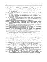
water level (Kollet and Maxwell, 2008). The predicted hydrologic change indicates
heterogeneous vulnerability of water resources and implies the associated impact on climate
change (Fig. 6).
Basin responses will also be accelerated by an ambitious project to divert water from the
Changjiang to the Yellow River, so-called, the South-to-North Water Transfer Project
(SNWTP) (Rich, 1983; Yang and Zehnder, 2001). It can be estimated that the degradation of
crop productivity may become severe, because most of the irrigation is dependent on
vulnerable water resources (McVicar et al., 2002). Further research is necessary to examine
the optimum amount of water that can be transferred, the effective management of the
Three Gorges Dam (TGD) in the Changjiang River, the overall economic and social
consequences of both projects, and their environmental assessment. It will be further
necessary to obtain more observed and statistical data relating to water level, soil and water
temperatures, water quality, and various phenological characteristics and crop productivity
of spring/winter wheat and summer maize, in addition to satellite data of higher
spatiotemporal resolution describing the seasonal and spatial vegetation phenology more
accurately. The linear relationship between evapotranspiration and biomass production,

Evapotranspiration – Remote Sensing and Modeling

140
which is very conservative and physiologically determined, is also valuable for further
evaluation of the relationship between changes in water use and crop production by
coupling with the numerical simulation and the satellite data analysis. Furthermore, it is
powerful to develop a more realistic mechanism for sub-models, and to predict future
hydrologic cycle and associated climate change using the model in order to achieve
sustainable development under sound socio-economic conditions.
4. Conclusion

This study coupled National Integrated Catchment-based Eco-hydrology (NICE) model
series with complex sub-models involving various factors, and clarified the importance of
and diverse water system in the highly cultivated Yellow River Basin, including
hydrological processes such as river dry-up, groundwater deterioration, agricultural water
use, et al. The model includes different functions of representative crops (wheat, maize,
soybean, and rice) and simulates automatically dynamic growth processes and biomass
formulation. The model reproduced reasonably evapotranspiration, irrigation water use,
groundwater level, and river discharge during spring/winter wheat and summer maize
cultivations. Scenario analysis predicted the impact of irrigation on both surface water and
groundwater, which had previously been difficult to evaluate. The simulated discharge with
irrigation was improved in terms of mean value, standard deviation, and coefficient of
variation. Because this region has experienced substantial river dry-up and groundwater
degradation at the end of the 20th century, this approach would help to overcome
substantial pressures of increasing food demand and declining water availability, and to
decide on appropriate measures for whole water resources management to achieve
sustainable development under sound socio-economic conditions.
5. Acknowledgment
The author thanks Dr. Y. Yang, Shijiazhuang Institute of Agricultural Modernization of the
Chinese Academy of Sciences (CAS), China, and Dr. M. Watanabe, Keio University, Japan,
for valuable comments about the study area. Some of the simulations in this study were run
on an NEC SX–6 supercomputer at the Center for Global Environmental Research (CGER),
NIES. The support of the Asia Pacific Environmental Innovation Strategy (APEIS) Project
and the Environmental Technology Development Fund from the Japanese Ministry of
Environment is also acknowledged.
6. References
Bondeau, A., Smith, P.C., Zaehle, S., Schaphoff, S., Lucht, W., Cramer, W., Gerten, D., Lotze-
Campen, H., Muller, C., Reichstein, M. & Smith, B. (2007) Modelling the role of
agriculture for the 20th century global terrestrial carbon balance. Global Change Biol.,
Vol.13, pp.679-706, doi: 10.1111/j.1365-2486.2006.01305.x, ISSN 1354-1013
Brown, L.R. & Halweil, B. (1998). China’s water shortage could shake world food security.

World Watch, July/August, Vol.11(4), pp.10-18

Impact of Irrigation on Hydrologic Change in Highly Cultivated Basin

141
Bugmann, H.K.M., Yan, X., Sykes, M.T., Martin, P., Linder, M., Desanker, P.V. & Cumming,
S.G. (1996) A comparison of forest gap models: model structure and behaviour.
Climatic Change, Vol.34, pp.289–313, ISSN 0165-0009
Cai, X. & Rosegrant, M.W. (2004). Optional water development strategies for the Yellow
River Basin: Balancing agricultural and ecological water demands. Water Resour.
Res., Vol.40, W08S04, doi: 10.1029/2003WR002488, ISSN 0043-1397
Cai, X. (2006). Water stress, water transfer and social equity in Northern China: Implication for
policy reforms. Human Development Report 2006, UNEP, Available from
ximing.pdf
Chen, J., He, D. & Cui, S. (2003a). The response of river water quality and quantity to the
development of irrigated agriculture in the last 4 decades in the Yellow River Basin,
China. Water Resour. Res., Vol.39(3), 1047, doi: 10.1029/2001WR001234, ISSN 0043-
1397
Chen, J.Y., Tang, C.Y., Shen, Y.J., Sakura, Y., Kondoh, A. & Shimada, J. (2003b). Use of water
balance calculation and tritium to examine the dropdown of groundwater table in
the piedmont of the North China Plain (NCP). Environ. Geol., Vol.44, pp.564-571,
ISSN 0943-0105
Chen, Y.M., Guo, G.S., Wang, G.X., Kang, S.Z., Luo, H.B. & Zhang, D.Z. (1995). Main crop
water requirement and irrigation of China. Hydrologic and Electronic Press, Beijing,
73-102
China Institute for Geo-Environmental Monitoring (CIGEM) (2003). China Geological
Envoronment Infonet, Database of groundwater observation in the People’s Republic of
China, Available from
Chinese Academy of Sciences (CAS) (1982). Topographic maps of 1:50,000 and 1:100,000
Chinese Academy of Sciences (CAS) (1988). Administrative division coding system of the

People’s Republic of China, Beijing
Chinese Academy of Sciences (CAS) (2003). China soil database, Available from

Clapp, R.B. & Hornberger, G.M. (1978). Empirical equations for some soil hydraulic
properties. Water Resour. Res., Vol.14, 601-604, ISSN 0043-1397
Cong, Z., Zhao, J., Yang, D. & Ni, G. (2010) Understanding the hydrological trends of river
basins in China. J. Hydrol., Vol.388, pp.350-356, doi: 10.1016/j.jhydrol.2010.05.013,
ISSN 0022-1694
Doll, P. & Siebert, S. (2002). Global modeling of irrigation water requirements. Water Resour.
Res., Vol.38, 8-1—8-10, ISSN 0043-1397
Entin, J.K., Robock, A., Vinnikov, K.Y., Hollinger, S.E., Liu, S. & Namkhai, A. (2000).
Temporal and spatial scales of observed soil moisture variations in the extratropics.
J. Geophys. Res., Vol.105(D9), pp.11865-11877, ISSN 0148-0227
Fang, W., Imura, H. & Shi, F. (2006). Wheat irrigation water requirement variability (2001-
2030) in the Yellow River Basin under HADCM3 GCM scenarios. Jpn. J. Environ.
Sci., Vol.19(1), pp.3-14
Fu, G., Chen, S., Liu, C. & Shepard, D. (2004). Hydro-climatic trends of the Yellow River
basin for the last 50 years. Climatic Change, Vol.65, pp.149-178, ISSN 0165-0009
Geological Atlas of China (2002). Geological Publisher, Beijing, China (in Chinese)

Evapotranspiration – Remote Sensing and Modeling

142
Godwin, D.C. & Jones, C.A. (1991). Nitrogen dynamics in soil-plant systems, In: Modeling
plant and soil systems, Hanks, R.J. & Ritchie, J.T. (Eds.), 287-321, Agronomy 31,
American Society of Agronomy, Madison, Wisconsin, USA
Hebei Department of Water Conservancy (1987). Hebei year book of water conservancy for 1987
(in Chinese)
Hebei Department of Water Conservancy (1988). Hebei year book of water conservancy for 1988
(in Chinese)

Hendrickson, O.Q., Fogal, W.H. & Burgess, D. (1990) Growth and resistance to herbivory in
N2-fixing alders. Can. J. Bot., Vol.69, pp.1919–1926, ISSN 0008-4026
Kollet, S.J., Maxwell, R.M., 2008. Capturing the influence of groundwater dynamics on land
surface processes using an integrated, distributed watershed model. Water Resour.
Res., Vol.44, W02402, doi: 10.1029/2007WR006004, ISSN 0043-1397
Lee, T.M. (1996). Hydrogeologic controls on the groundwater interactions with an acidic
lake in karst terrain, Lake Barco, Florida. Water Resour. Res., Vol.32, 831-844, ISSN
0043-1397
Liu, C., Zhang, X. & Zhang, Y. (2002). Determination of daily evapotranspiration of winter
wheat and corn by large-scale weighting lysimeter and micro-lysimeter. Agr. Forest.
Meteorol., Vol.111, pp.109-120, ISSN 0168-1923
Liu, C. & Xia, J. (2004). Water problems and hydrological research in the Yellow River and
the Huai and Hai River basins of China. Hydrol. Process., Vol.18, pp.2197-2210, doi:
10.1002/hyp.5524, ISSN 0885-6087
Liu, C. & Zheng, H. (2004). Changes in components of the hydrological cycle in the Yellow
River basin during the second half of the 20th century. Hydrol. Process., Vol.18,
pp.2337-2345, doi: 10.1002/hyp.5534, ISSN 0885-6087
Liu, J.Y. (1996). Macro-scale survey and dynamic study of natural resources and environment of
China by remote sensing, Chinese Science and Technology Publisher, Beijing, China
(in Chinese)
Liu, L., Yang, Z. & Shen, Z. (2003). Estimation of water renewal times for the middle and
lower sections of the Yellow River. Hydrol. Process., Vol.17, pp.1941-1950, doi:
10.1002/hyp.1219, ISSN 0885-6087
Maxwell, R.M. & Kollet, S.J. (2008). Interdependence of groundwater dynamics and land-
energy feedbacks under climate change. Nat. Geosci., Vol.1, pp.665-669, doi:
10.1038/ngeo315, ISSN 1752-0894
McVicar, T.R., Zhang, G.L., Bradford, A.S., Wang, H.X., Dawes, W.R., Zhang, L. & Li, L.
(2002). Monitoring regional agricultural water use efficiency for Hebei Province on
the North China Plain. Aust. J. Agric. Res., Vol.53, pp.55-76, ISSN 0004-9409
Nakayama, T. & Watanabe, M. (2004). Simulation of drying phenomena associated with

vegetation change caused by invasion of alder (Alnus japonica) in Kushiro Mire.
Water Resour. Res., Vol.40, W08402, doi: 10.1029/2004WR003174, ISSN 0043-1397
Nakayama, T. & Watanabe, M. (2006). Simulation of spring snowmelt runoff by considering
micro-topography and phase changes in soil layer. Hydrol. Earth Syst. Sci. Discuss.,
Vol.3, pp.2101-2144, ISSN 1027-5606
Nakayama, T., Yang, Y., Watanabe, M. & Zhang, X. (2006). Simulation of groundwater
dynamics in North China Plain by coupled hydrology and agricultural models.
Hydrol. Process., Vol.20(16), pp.3441-3466, doi: 10.1002/hyp.6142, ISSN 0885-6087

Impact of Irrigation on Hydrologic Change in Highly Cultivated Basin

143
Nakayama, T., Watanabe, M., Tanji, K. & Morioka, T. (2007). Effect of underground urban
structures on eutrophic coastal environment. Sci. Total Environ., Vol.373(1), pp.270-
288, doi: 10.1016/j.scitotenv.2006.11.033, ISSN 0048-9697
Nakayama, T. (2008a). Factors controlling vegetation succession in Kushiro Mire. Ecol.
Model., Vol.215, pp.225-236, doi: 10.1016/j.ecolmodel.2008.02.017, ISSN 0304-3800
Nakayama, T. (2008b). Shrinkage of shrub forest and recovery of mire ecosystem by river
restoration in northern Japan. Forest Ecol. Manag., Vol.256, pp.1927-1938, doi:
10.1016/j.foreco.2008.07.017, ISSN 0378-1127
Nakayama, T. & Watanabe, M. (2008a). Missing role of groundwater in water and nutrient
cycles in the shallow eutrophic Lake Kasumigaura, Japan. Hydrol. Process., Vol.22,
pp.1150-1172, doi: 10.1002/hyp.6684, ISSN 0885-6087
Nakayama, T. & Watanabe, M. (2008b). Role of flood storage ability of lakes in the
Changjiang River catchment. Global Planet. Change, Vol.63, pp.9-22, doi:
10.1016/j.gloplacha.2008.04.002, ISSN 0921-8181
Nakayama, T. & Watanabe, M. (2008c). Modelling the hydrologic cycle in a shallow
eutrophic lake. Verh. Internat. Verein. Limnol., Vol.30
Nakayama, T. (2009). Simulation of Ecosystem Degradation and its Application for Effective
Policy-Making in Regional Scale, In: River Pollution Research Progress, Mattia N.

Gallo & Marco H. Ferrari (Eds.), 1-89, Nova Science Publishers, Inc., ISBN 978-1-
60456-643-7, New York
Nakayama, T. (2010). Simulation of hydrologic and geomorphic changes affecting a
shrinking mire. River Res. Appl., Vol.26(3), pp.305-321, doi: 10.1002/rra.1253, ISSN
1535-1459
Nakayama, T. & Fujita, T. (2010). Cooling effect of water-holding pavements made of new
materials on water and heat budgets in urban areas. Landscape Urban Plan., Vol.96,
pp.57-67, doi: 10.1016/j.landurbplan.2010.02.003, ISSN 0169-2046
Nakayama, T., Sun, Y. & Geng, Y. (2010). Simulation of water resource and its relation to
urban activity in Dalian City, Northern China. Global Planet. Change, Vol.73, pp.172-
185, doi: 10.1016/j.gloplacha.2010.06.001, ISSN 0921-8181
Nakayama, T. (2011a). Simulation of complicated and diverse water system accompanied by
human intervention in the North China Plain. Hydrol. Process., Vol.25, pp.2679-2693
doi: 10.1002/hyp.8009, ISSN 0885-6087
Nakayama, T. (2011b). Simulation of the effect of irrigation on the hydrologic cycle in the
highly cultivated Yellow River Basin. Agr. Forest Meteorol., Vol.151, pp.314-327, doi:
10.1016/j.agrformet.2010.11.006, ISSN 0168-1923
Nakayama, T. & Hashimoto, S. (2011). Analysis of the ability of water resources to reduce
the urban heat island in the Tokyo megalopolis. Environ. Pollut., Vol.159, pp.2164-
2173, doi: 10.1016/j.envpol.2010.11.016, ISSN 0269-7491
Nakayama, T., Hashimoto, S. & Hamano, H. (2011). Multi-scaled analysis of hydrothermal
dynamics in Japanese megalopolis by using integrated approach. Hydrol. Process.
(in press), ISSN 0885-6087
Nash, J.E. & Sutcliffe, J.V. (1970). Riverflow forecasting through conceptual model. J. Hydrol.,
Vol.10, pp.282-290, ISSN 0022-1694
Oleson, K.W., Niu, G Y., Yang, Z L., Lawrence, D.M., Thornton, P.E., Lawrence, P.J.,
Stockli, R., Dickinson, R.E., Bonan, G.B., Levis, S., Dai, A. & Qian, T. (2008)

Evapotranspiration – Remote Sensing and Modeling

144
Improvements to the Community Land Model and their impact on the hydrological
cycle. J. Geophys. Res., Vol.113, G01021, doi: 10.1029/2007JG000563, ISSN 0148-0227
Oreskes, N., Shrader-Frechette, K. & Belitz, K. (1994). Verification, validation, and
confirmation of numerical models in the earth sciences. Science, Vol.263, pp.641-646,
ISSN 0036-8075
Priestley C.H.B. & Taylor, R.J. (1972). On the assessment of surface heat flux and
evaporation using large-scale parameters. Mon. Weather Rev., Vol.100, pp.81-92,
ISSN 0027-0644
Rawls, W.J., Brakensiek, D.L. & Saxton, K.E. (1982). Estimation of soil water properties.
Trans. ASAE, Vol.25, pp.1316-1320
Ren, L., Wang, M., Li, C. & Zhang, W. (2002). Impacts of human activity on river runoff in
the northern area of China. J. Hydrol., Vol.261, pp.204-217, ISSN 0022-1694
Rich, V. (1983). Yangtze to cross Yellow River. Nature, Vol.305, pp.568, ISSN 0028-0836
Ritchie, J.T., Singh, U., Godwin, D.C. & Bowen, W.T. (1998). Cereal growth, development
and yield, In: Understanding Options for Agricultural Production, Tsuji, G.Y.,
Hoogenboom, G. & Thornton, P.K. (Eds.), 79-98, Kluwer, ISBN 0-7923-4833-8, Great
Britain
Robock, A., Konstantin, Y.V., Govindarajalu, S., Jared, K.E., Steven, E.H., Nina, A.S., Suxia,
L. & Namkhai, A. (2000). The global soil moisture data bank. Bull. Am. Meteorol.
Soc., Vol.81, pp.1281-1299, Available from

Roderick, M.L. & Farquhar, G.D. (2002) The cause of decreased pan evaporation over the
past 50 years. Science, Vol.298(15), pp.1410-1411, ISSN 0036-8075
Sato, Y., Ma, X., Xu, J., Matsuoka, M., Zheng, H., Liu, C. & Fukushima, Y. (2008). Analysis of
long-term water balance in the source area of the Yellow River basin. Hydrol.
Process., Vol.22, pp.1618-1929, doi: 10.1002/hyp.6730, ISSN 0885-6087
Sellers, P.J., Randall, D.A., Collatz, G.J., Berry, J.A., Field, C.B., Dazlich, D.A., Zhang, C.,
Collelo, G.D. & Bounoua, L. (1996). A revised land surface prameterization (SiB2)
for atomospheric GCMs. Part I : Model formulation. J. Climate, Vol.9, pp.676-705,

ISSN 0894-8755
Shimada, J. (2000). Proposals for the groundwater preservation toward 21st century through
the view point of hydrological cycle. J. Japan Assoc. Hydrol. Sci., Vol.30, pp.63-72 (in
Japanese)
Sun, R., Gao, X., Liu, C.M. & Li, X.W. (2004). Evapotranspiration estimation in the Yellow
River Basin, China using integrated NDVI data. Int. J. Remote Sens., Vol.25, pp.2523-
2534, ISSN 0143-1161
Tang, Q., Oki, T., Kanae, S. & Hu, H. (2007). The influence of precipitation variability and
partial irrigation within grid cells on a hydrological simulation. J. Hydrometeorol.,
Vol.8, pp.499-512, doi: 10.1175/JHM589.1, ISSN 1525-755X
Tang, Q., Oki, T., Kanae, S. & Hu, H. (2008a). Hydrological cycles change in the Yellow
River basin during the last half of the twentieth century. J. Climate, Vol.21, pp.1790-
1806, doi: 10.1175/2007JCLI1854.1, ISSN 0894-8755
Tang, Q., Oki, T., Kanae, S. & Hu, H. (2008b). A spatial analysis of hydro-climatic and
vegetation condition trends in the Yellow River basin. Hydrol. Process., Vol.22,
pp.451-458, doi: 10.1002/hyp.6624, ISSN 0885-6087

Impact of Irrigation on Hydrologic Change in Highly Cultivated Basin

145
Tao, F., Yokozawa, M., Xu, Y., Hayashi, Y. & Zhang, Z. (2006). Climate changes and trends
in phenology and yields of field crops in China, 1981-2000. Agr. Forest Meteorol.,
Vol.138, pp.82-92, ISSN 0168-1923
U.S. Geological Survey (USGS) (1996). GTOPO30 Global 30 Arc Second Elevation Data Set,
USGS, Available from
gtopo30.html
Wang, H., Zhang, L., Dawes, W.R. & Liu, C. (2001). Improving water use efficiency of
irrigated crops in the North China Plain – measurements and modeling. Agr. Forest.
Meteorol., Vol.48, pp.151-167, ISSN 0168-1923
Xia, J., Wang, Z., Wang, G. & Tan, G. (2004). The renewability of water resources and its

quantification in the Yellow River basin, China. Hydrol. Process., Vol.18, pp.2327-
2336, doi: 10.1002/hyp.5532, ISSN 0885-6087
Xu, Z.X., Takeuchi, K., Ishidaira, H. & Zhang, X.W. (2002). Sustainability analysis for Yellow
River Water Resources using the system dynamics approach. Water Resour. Manag.,
Vol.16, pp.239-261, ISSN 0920-4741
Yang, Z.S., Milliman, J.D., Galler, J., Liu, J.P. & Sun, X.G. (1998). Yellow River’s water and
sediment discharge decreasing steadily. EOS, Vol.79(48), pp.589-592, ISSN 0096-
3941
Yang, H. & Zehnder, A. (2001). China’s regional water scarcity and implications for grain
supply and trade. Environ. Plann. A, Vol.33, pp.79-95
Yang, D. & Musiake, K. (2003). A continental scale hydrological model using the distributed
approach and its application to Asia. Hydrol. Process., Vol.17, pp.2855-2869, doi:
10.1002/hyp.1438, ISSN 0885-6087
Yang, D., Li, C., Hu, H., Lei, Z., Yang, S., Kusuda, T., Koike, T. & Musiake, K. (2004a).
Analysis of water resources variability in the Yellow River of China during the last
half century using historical data. Water Resour. Res., Vol.40, W06502, doi:
10.1029/2003WR002763, ISSN 0043-1397
Yang, H.S., Dobermann, A., Lindquist, J.L., Walters, D.T., Arkebauer, T.J. & Cassman, K.G.
(2004b) Hybrid-maize–a maize simulation model that combines two crop modeling
approaches. Field Crop. Res., Vol.87, pp.131-154, ISSN 0378-4290
Yellow River Conservancy Commission (1987). Annual report of discharge and sediment in
Yellow River, Interior report of the committee (in Chinese)
Yellow River Conservancy Commission (1988). Annual report of discharge and sediment in
Yellow River, Interior report of the committee (in Chinese)
Yellow River Conservancy Commission (2002). Yellow River water resources bulletins,
Available from (in Chinese)
Zhang, J., Huang, W.W. & Shi, M.C. (1990). Huanghe (Yellow River) and its estuary:
sediment origin, transport and deposition. J. Hydrol., Vol.120, pp.203-223, ISSN
0022-1694
Zhou, M.C., Ishidaira, H. & Takeuchi, K. (2007). Estimation of potential

evapotranspiration over the Yellow River basin: reference crop evaporation or
Shuttleworth-Wallance?. Hydrol. Process., Vol.21, pp.1860-1874, doi:
10.1002/hyp.6339, ISSN 0885-6087

Evapotranspiration – Remote Sensing and Modeling

146
Zhu, Y. (1992). Comprehensive hydro-geological evaluation of the Huang-Huai-Hai Plain,
Geological Publishing House of China, 277p., Beijing, China (in Chinese)
8
Estimation of Evapotranspiration Using
Soil Water Balance Modelling
Zoubeida Kebaili Bargaoui
Tunis El Manar University
Tunisia
1. Introduction
Assessing evapotranspiration is a key issue for natural vegetation and crop survey. It is a
very important step to achieve the soil water budget and for deriving drought awareness
indices. It is also a basis for calculating soil-atmosphere Carbon flux. Hence, models of
evapotranspiration, as part of land surface models, are assumed as key parts of hydrological
and atmospheric general circulation models (Johnson et al., 1993). Under particular climate
(represented by energy limiting evapotranspiration rate corresponding to potential
evapotranspiration) and soil vegetation complex, evapotranspiration is controlled by soil
moisture dynamics. Although radiative balance approaches are worth noting for
evapotranspiration evaluation, according to Hofius (2008), the soil water balance seems the
best method for determining evapotranspiration from land over limited periods of time.
This chapter aims to discuss methods of computing and updating evapotranspiration rates
using soil water balance representations.
At large scale, Budyko (1974) proposed calculating annual evapotranspiration from data of
meteorological stations using one single parameter w

0
representing a critical soil water
storage. Using a statistical description of the sequences of wet and dry days, Eagleson (1978
a) developed an average annual water balance equation in terms of 23 variables including
soil, climate and vegetation parameters with the assumption of a homogeneous soil-
atmosphere column using Richards (1931) equation. On the other hand, the daily bucket
with bottom hole model (BBH) proposed by Kobayashi et al. (2001) was introduced based
on Manabe model (1969) involving one single layer bucket but including gravity drainage
(leakage) as well as capillary rise. Vrugt et al. (2004) concluded that the daily Bucket model
and the 3-D model (MODHMS) based on Richards equation have similar results. Also,
Kalma & Boulet (1998) compared simulation results of the rainfall runoff hydrological
model VIC which assumes a bucket representation including spatial variability of soil
parameters to the one dimensional physically based model SiSPAT (Braud et al. , 1995).
Using soil moisture profile data for calibration, they conclude that catchment’s scale wetness
index for very dry and very wet periods are misrepresented by SiSPAT while captured by
VIC. Analyzing VIC parameter identifiability using streamflow data, DeMaria et al. (2007)
concluded that soil parameters sensitivity was more strongly dictated by climatic gradients
than by changes in soil properties especially for dry environments. Also, studying the
measurements of soil moisture of sandy soils under semi-arid conditions, Ceballos et al.
(2002) outlined the dependence of soil moisture time series on intra annual rainfall

Evapotranspiration – Remote Sensing and Modeling

148
variability. Kobayachi et al. (2001) adjusted soil humidity profiles measurements for model
calibration while Vrugt et al. (2004) suggested that effective soil hydraulic properties are
poorly identifiable using drainage discharge data.
The aim of the chapter is to provide a review of evapotranspiration soil water balance
models. A large variety of models is available. It is worth noting that they do differ with
respect to their structure involving empirical as well as conceptual and physically based

models. Also, they generally refer to soil properties as important drivers. Thus, the chapter
will first focus on the description of the water balance equation for a column of soil-
atmosphere (one dimensional vertical equation) (section 2). Also, the unsaturated
hydrodynamic properties of soils as well as some analytical solutions of the water balance
equation are reviewed in section 2. In section 3, key parameterizations generally adopted to
compute actual evapotranspiration will be reported. Hence, several soil water balance
models developed for large spatial and time scales assuming the piecewise linear form are
outlined. In section 4, it is focused on rainfall-runoff models running on smaller space scales
with emphasizing on their evapotranspiration components and on calibration methods.
Three case studies are also presented and discussed in section 4. Finally, the conclusions are
drawn in section 5.
2. The one dimensional vertical soil water balance equation
As pointed out by Rodriguez-Iturbe (2000) the soil moisture balance equation (mass
conservation equation) is “likely to be the fundamental equation in hydrology”. Considering
large spatial scales, Sutcliffe (2004) might agree with this assumption. In section 2.1 we first
focus on the presentation of the equation relating relative soil moisture content to the water
balance components: infiltration into the soil, evapotranspiration and leakage. Then water
loss through vegetation is addressed. Finally, infiltration models are discussed in section 2.2.
2.1 Water balance
For a control volume composed by a vertical soil column, the land surface, and the
corresponding atmospheric column, and under solar radiation and precipitation as forcing
variables, this equation relates relative soil moisture content s to infiltration into the soil
I(s,t), evapotranspiration E(s,t) and leakage L(s,t).
nZ
a
st= I(s,t) – E(s,t) – L(s,t) (1a)
Where t is time, n is soil effective porosity (the ratio of volume of voids to the total soil
matrix volume); and Z
a
is the active depth of soil.

Soil moisture exchanges as well as surface heat exchanges depend on physical soil
properties and vegetation (through albedo , soil emissivity, canopy conductance) as well as
atmosphere properties (turbulent temperature and water vapour transfer coefficients,
aerodynamic conductance in presence of vegetation) and weather conditions (solar
radiation, air temperature, air humidity, cloud cover, wind speed). Soil moisture
measurements require sampling soil moisture content by digging or soil augering and
determining soil moisture by drying samples in ovens and measuring weight losses; also, in
situ use of tensiometry, neutron scattering, gamma ray attenuation, soil electrical
conductivity analysis, are of common practice (Gardner et al. (2001) ; Sutcliffe, 2004; Jeffrey
et al. (2004) ).

Estimation of Evapotranspiration Using Soil Water Balance Modelling

149
The basis of soil water movement has been experimentally proposed by Darcy in 1856 and
expresses the average flow velocity in a porous media in steady-state flow conditions of
groundwater. Darcy introduced the notion of hydraulic conductivity. Boussinesq in 1904
introduced the notion of specific yield so as to represent the drainage from the unsaturated
zone to the flow in the water table. The specific yield is the flux per unit area draining for a
unit fall in water table height. Richards (1931) proposed a theory of water movement in the
unsaturated homogeneous bare soil represented by a semi infinite homogeneous column:
/t= /z [ K /z – K()] (1b)
Where t is time;  is volumetric water content (which is the ratio between soil moisture
volume and the total soil matrix volume cm
3
cm
-3
); z is the vertical coordinate (z>0
downward from surface); K is hydraulic conductivity (cms
-1

);  is the soil water matrix
potential. Both K and are function of the volumetric water content. Richards equation
assumes that the effect of air on water flow is negligible. If accounting for the slope surface,
it comes:
tzzzcos 
Where is surface slope angle and cos is the cosinus function. We notice that the term [K
/z – K()] represents the vertical moisture flux. In particular, as reported by Youngs
(1988) the soil-water diffusivity parameter D has been proposed by Childs and Collis-
George (1950) as key soil-water property controlling the water movement.
D 
Thus, the Richards equation is often written as following:
tzDz–z 
Eq. (4) is generally completed by source and sink terms to take into account the occurrence
of precipitation infiltrating into the soil I
nf
(,z
0
) where z
0
is the vertical coordinate at the
surface and vegetation uptake of soil moisture g
r
(,z),. Vegetation uptake (transpiration)
depends on vegetation characteristics (species, roots, leaf area, and transfer coefficients) and
on the potential rate of evapotranspiration E
0
which characterizes the climate. Consequently,
Eq. (4) becomes:
t= z [ D(z - K()] –g
r

(,z) + I
nf
(,z
0
) (5)
Youngs (1988) noticed that near the soil surface where temperature gradients are important
Richards equation may be inadequate. We find in Raats (2001) an important review of
evapotranspiration models and analytical and numerical solutions of Richards equation.
However, it should be noticed that after Feddes et al. (2001) “in case of catchments with
complex sloping terrain and groundwater tables, a vertical domain model has to be coupled
with either a process or a statistically based scheme that incorporates lateral water transfer”.
So, a key task in the soil water balance model evaluation is the estimation of I
nf
(,z
0
) and
g
r
(,z). Both depend on the distribution of soil moisture. We focus here on vegetation uptake
(or transpiration) g
r
(,z) which is regulated by stomata and is driven by atmospheric
demand. Based on an Ohm’s law analogy which was primary proposed by Honert in 1948
as outlined by Eagleson (1978 b), the conceptual model of local transpiration uptake u(z,t)=
g
r
(,z) as volume of water per area per time is expressed as (Guswa, 2005)

Evapotranspiration – Remote Sensing and Modeling

150
u(z,t)=z (z,t) -
p
) /[ R
1
( (z,t))+R
2
] (6)
soil moisture potential (bars), 
p
leaf moisture potential (bars); R
1
(s cm
-1
) a resistance to
moisture flow in soil; it depends on soil and root characteristics and is function of the
volumetric water content; R
2
(s cm
-1
) is vegetation resistance to moisture flow; z is soil
depth. It is worth noting that 
p
>  where  is the wilting point potential; In Ceballos et
al. (2002) the wilting point is taken as the soil-moisture content at a soil-water potential of -
1500 kPa.
Estimations of air and canopy resistances R
1
and R
2

often use semi-empirical models based
on meteorological data such as wind speed as explanatory variables (Monteith (1965);
Villalobos et al., 2000). Jackson et al. (2000) pointed out the role of the Hydraulic Lift process
which is the movement of water through roots from wetter, deeper soil layers into drier,
shallower layers along a gradient in . On the basis of such redistribution at depth, Guswa
(2005) introduced a parameter to represent the minimum fraction of roots that must be
wetted to the field capacity in order to meet the potential rate of transpiration. The field
capacity is defined as the saturation for which gravity drainage becomes negligible relative
to potential transpiration (Guswa, 2005). The potential matrix at field capacity is assumed
equal to 330 hPa (330 cm) (Nachabe, 1998). The resulting u(z,t) function is strongly non
linear versus the average root moisture with a relative insensitivity to changes in moisture
when moisture is high and sensitivity to changes in moisture when the moisture is near the
wilting point conditions. We also emphasize the Perrochet model (Perrochet, 1987) which
links transpiration to potential evapotranspiration E
0
through:
g
r
(,z,t) = (r(z) E
0
(t) (7)
Where r(z) (cm
-1
) is a root density function which depends both on vegetation type and
climatic conditions, (is the root efficiency function. Both r(z) and (represent
macroscopic properties of the root soil system; they depend on layer thickness and root
distribution . Lai and Katul (2000) and Laio (2006) reported some models assigned to r(z)
which are linear or non linear. As out pointed by Laio (2006), models generally assume that
vegetation uptake at a certain depth depends only on the local soil moisture. It is noticeable
that in Feddes et al. (2001), a decrease of uptake is assumed when the soil moisture exceeds

a certain limit and transpiration ceases for soil moisture values above a limit related to
oxygen deficiency.
2.2 Review of models for hydrodynamic properties of soils
Many functional forms are proposed to describe soil properties evolution as a function of
the volumetric water content (Clapp et al. , 1978). They are called retention curves or pedo
transfer functions. We first present the main functional forms adopted to describe hydraulic
parameters (section 2.2.1). Then, we report some solutions of Richards equation (section
2.2.2).
2.2.1 Functional forms of soil properties
According to Raats (2001), four classes of models are distinguishable for representing soil
hydraulic parameters. Among them the linear form with D as constant and K linear with
and the function Delta type as proposed by Green Ampt D= ½ s² (
1
- 
0
)
-1
(
1
- 
0
) where
s is the degree of saturation (which is the ratio between soil moisture volume and voids

Estimation of Evapotranspiration Using Soil Water Balance Modelling

151
volume; s=1 in case of saturation) and 
1
; 

0
parameters. Also power law functions for 
and K) are proposed by Brooks and Corey (1964) on the basis of experimental
observations while Gardner (1958) assumes exponential functions.

The power type model
proposed by Brooks & Corey (1964) are the most often adopted forms in rainfall-runoff
transformation models. The Brooks and Corey model for K and is written as:
K(s) = K

(1) s
c’
;  (s) = (1) s
-1/m
(8)
where m is a pore size index and c’ a pore disconnectedness index (Eagleson 1978 a,b); After
Eagleson (1978a, b), c’ is linked to m with c’=(2+3m)/m. In Eq. (8), K(1) is hydraulic
conductivity at saturation (for s=1); (1) is the bubbling pressure head which represents
matrix potential at saturation. During dewatering of a sample, it corresponds to the suction
at which gas is first drawn from the sample; As a result, Brooks and Corey (BC) model for
diffusivity is derived as:
Ds
d
 K

(1) /(nm) (9)
where n is effective soil porosity; and d=(c’-1- (1/m)). Let’s consider the intrinsic
permeability k which is a soil property. (K and k are related by K= k
w
 where dynamic

viscosity of water; 
w
specific weight of pore water). After Eagleson (1978 a, b), three
parameters involved in pedo transfer functions may be considered as independent
parameters: n, c’ and k(1) where k(1) is intrinsic permeability at saturation.
On the other hand, Gardner (1958) model assumed the exponential form for the hydraulic
conductivity parameter (Eq. 10):
K= K
S
e
–a’


Where K
S
saturated hydraulic conductivity at soil surface; a’ pore size distribution
parameter. Also, in Gardner (1958) model, the degree of saturation and the soil moisture
potential are linked according to Eq. (11). The power function introduces a parameter l
which is a factor linked to soil matrix tortuosity (l= 0.5 is recommended for different types of
soils);.
s() = [e
-0.5 a’

(1+ 0.5 a’ )]
2/(l+2)
(11)
Van Genutchen model (1980) is another kind of power law model but it is highly non linear
K= K
S
s



[ 1- (1- s
(

)

]² (12)
s= [1+ (


]
-

for ≤
s=1 for 


In Eq. (12) and (13)  is a parameter to be calibrated. Calibration is generally performed on
the basis of the comparison of computed and observed retention curves.
In order to determine K
S
one way is to adopt Cosby et al. (1984) model (Eq. 14).
Log(K
S
0. 6 ( 0.0126 S
%
– 0.0064 C
%
) (14)

Where S
%
and C
%
stand for soil percents of sand and clay. Also, we may find tabulated
values of K
S
(in m/day) according to soil texture and structure properties in FAO (1980). On

Evapotranspiration – Remote Sensing and Modeling

152
the other hand, soil field capacity S
FC
plays a key role in many soil water budget models. In
Ceballos et al. (2002) the field capacity was considered as “the content in humidity
corresponding to the inflection point of the retention curve before it reached a trend parallel
to the soil water potential axis”. In Guswa (2005), it is defined as the saturation for which
gravity drainage becomes negligible relative to potential transpiration. As pointed out by
Liao (2006) who agreed with Nachabe (1998), there is an “intrinsic subjectivity in the
definition of field capacity”. Nevertheless, many semi-empirical models are offered in the
literature for S
FC
estimation as a function of soil properties (Nachabe, 1988). In Cosby (1984),
S
FC
expressed as a degree of saturation is assumed s:
S
FC
= 50.1 + (-0.142 S

%
- 0.037 C
%
) (15)
On the other hand, according to Cosby (1984) and Saxton et al. (1986) S
FC
may be derived as:
S
FC
= (20/A’)
1/B’
(16)
where
A’=100*exp(a
1
+a
2
C
%
+a
3
S
%
2
+a
4
S
%
2
C

%
); B’=a
5
+a
6
C
%
2
+a
7
S
%
2
+a
8
S
%
2
C
%
; a
1
= - 4,396; a
2
= - 0,0715; a
3

= - 0,000488; a
4
= -0,00004285; a

5
= -0,00222; a
6
= -0,00222 ; a
7
= -0,00003484; a
8
= -0,00003484
Recently, this model was adopted by Zhan et al. (2008) to estimate actual evapotranspiration
in eastern China using soil texture information. Also, soil characteristics such as S
FC
may be
obtained from Rawls & Brakensiek (1989) according to soil classification (Soil Survey
Division Staff, 1998). Nasta et al. (2009) proposed a method taking advantage of the
similarity between shapes of the particle-size distribution and the soil water retention
function and adopted a log-Normal Probability Density Function to represent the matrix
pressure head function retention curve.
2.2.2 Review of analytical solutions of the movement equation
Two well-known solutions of Richards equation are reported here (Green &Ampt model
(1911), Philip model (1957)) as well as a more recent solution proposed by Zhao and Liu
(1995). These solutions are widely adopted in rainfall-runoff models to derive
infiltration.
In the Green &Ampt method (1911), it is assumed that infiltration capacity f from a ponded
surface is:
f 
av
( 1 + F

) (17)


av
average saturated hydraulic conductivity ; difference in average matrix potential
before and after wetting;  difference in average soil water content before and after
wetting; F the cumulative infiltration for a rainfall event (with f = dF/dt).
In the Philip (1957) solution, it is assumed that the gravity term is negligible so that
K()/z]≈0. A time series development considers the soil water profile of the form:
z(,t) = f
1
() t
1/2
+ f
2
() t + f
3
() t
3/2
+… (18)
Where f
1
, f
2
, … are functions of . Hence, the cumulative infiltration 
f
(t) is:

f
(t)= S t
1/2
+ (A
2

+K
S
) t + A
3
t
3/2
+ … (19)
Where S soil sorptivity, K
S
is saturated hydraulic conductivity of the soil and A
1
, A
2
, … are
parameters. Philip suggested adopting a truncation that results in:

Estimation of Evapotranspiration Using Soil Water Balance Modelling

153

f
(t)= S t
1/2
+ K
S
/n’ t (20)
Where n’ is a factor 0.3 < n’ < 0.7. It is worth noting that the soil sorptivity S depends on
initial water content. So it has to be adjusted for each rainfall event. This is usually
performed by comparing observed and simulated cumulative infiltration. For further
discussion of Philip model, the reader may profitably refer to Youngs (1988).

Another model of infiltration is worth noting. It is the model of Zhao and Liu (1995) which
introduced the fraction of area under the infiltration capacity:
i(t)= i
max
[1- (1-A(t))
1/b’’
] (21)
Where i(t) is infiltration capacity at time t. Its maximum value is i
max
. A(t) is the fraction of
area for which the infiltration capacity is less than i(t) and b’’ is the infiltration shape
parameter. As out pointed by DeMaria et al. (2007), the parameter b’’ plays a key role.
Effectively, an increase in b’’ results in a decrease in infiltration.
3. Review of various parameterizations of actual evapotranspiration
Many early works on radiative balance combination methods for estimating latent heat
using Penman – Monteith method (Monteith, 1965) were coupled with empirical models for
representing the conductance of the soil-plant system (the conductance is the inverse
function of the resistance). Based on observational evidence, these works have assumed a
linear piecewise relation between volumetric soil moisture and actual evapotranspiration.
Thus, several water balance models have been developed for large spatial and time scales
assuming this piecewise linear form beginning from the work of Budyko in 1956 as pointed
out by Manabe (1969)), Budyko (1974), Eagleson (1978 a, b), Entekhabi & Eagleson (1989)
and Milly (1993). In fact, soil water models for computing actual evapotranspiration differ
according to the time and space scales and the number of soil layers adopted as well as the
degree of schematization of the water and energy balances. Moreover, specific canopy
interception schemes, pedo transfer sub-models and runoff sub-models often distinguish
between actual evapotranspiration schemes. Also, models differ by the consideration of
mixed bare soil and vegetation surface conditions or by differencing between vegetation and
soil cover. In the former, there is a separation between bare soil evapotranspiration and
vegetation transpiration as distinct terms in the computation of evapotranspiration. In the

following, we first present a brief review of land surface models which fully couple
energy and mass transfers (section 3.1). Then, we make a general presentation of soil
water balance models based on the actualisation of soil water storage in the upper soil
zone assuming homogeneous soil (section 3.2).Further, it is focused on the estimation of
long term actual evapotranspiration using approximation of the solution of the water
balance model (section 3.3). In section 3.4, large scale soil water balance models (bucket
schematization) are outlined with much more details. Finally a discussion is performed in
section 3.5.
3.1 Review of land surface models
In Soil-Vegetation-Atmosphere-Transfer (SVAT) models or land surface models, energy and
mass transfers are fully coupled solving both the energy balance (net radiation equation, soil
heat fluxes, sensible heat fluxes, and latent heat fluxes) in addition to water movement
equations. Usually this is achieved using small time scales (as for example one hour time

Evapotranspiration – Remote Sensing and Modeling

154
increment). The specificity of SVAT models is to describe properly the role of vegetation in
the evolution of water and energy budgets. This is achieved by assigning land type and soil
information to each model grid square and by considering the physiology of plant uptake.
Many SVAT models have been developed in the last 25 years. We may find in Dickinson
and al. (1986) perhaps one of the first comprehensive SVAT models which was addressed to
be used for General circulation modelling and climate modelling. It was called BATS
(Biosphere-Atmosphere Transfer Scheme). It was able to compute surface temperature in
response to solar radiation, water budget terms (soil moisture, evapotranspiration and,
runoff), plant water budget (interception and transpiration) and foliage temperature. ISBA
model (Noilhan et Mahfouf, 1996) was further developed in France and belongs to “simple
models with mono layer energy balance combined with a bulk soil description” (after Olioso
et al. (2002)). An example of using ISBA scheme is presented in Olioso et al. (2002). The
following variables are considered: surface temperature, mean surface temperature, soil

volumetric moisture at the ground surface, total soil moisture, canopy interception
reservoir. The soil volumetric moisture at the ground surface is adopted to compute the soil
evaporation while the total soil moisture is used to compute transpiration. The total latent
heat is assumed as a weighted average between soil evaporation and transpiration using a
weight coefficient depending on the degree of canopy cover. Canopy albedo and emissivity,
vegetation Leaf area index LAI, stomatal resistance, turbulent heat and transfer coefficients
are parameters of the energy balance equations. It is worth noting that soil parameters in
temperature and moisture are computed using soil classification databases. Without loss of
generality we briefly present the two layers water movement model adopted by Montaldo
et al. (2001)

g
t= C
1
/ (
w
d
1
) [ P
g
-E
g
] –C
2
/ [
g
-
geq
] 0≤
g

≤
s
(22)

2
t= C
1
/ (
w
d
2
) [ P
g
-E
g
–E
tr
– q
2
] 0≤
2
≤
s
(23)
d
1
and d
2
depth of near surface and root zone soil layers; 
w

density of the water; 
g
and 
2

volumetric water contents of near surface and root zone soil layers; 
geq
equilibrium surface
volumetric soil moisture content ideally describing a reference soil moisture for which
gravity balances capillary forces such that no flow crosses the bottom of the near surface
zone of depth d
1
; P
g
precipitation infiltrating into the soil; E
g
bare soil evaporation rate at the
surface; E
tr
transpiration rate from the root zone of depth d
2
; q
2
rate of drainage out of the
bottom of the root zone; It is assumed to be equal to the hydraulic conductivity of the root
zone at =
2
 ; C
1
and C

2
are parameters. In this model, the rescaling of the root zone soil
moisture 
2
seems to be highly recommended in order to achieve adequate prediction of 
g

in comparison to observations (Montaldo et al. (2001)). Using an assimilation procedure,
Montaldo et al. (2001) achieved overcoming misspecification of K
S
of two orders magnitude
in the simulation of 
2
.
According to Franks et al. (1997), the calibration of SVAT schemes requires a large number
of parameters. Also, field experimentations needed to calibrate these parameters are rather
important. Moreover up scaling procedures are to be implemented. Boulet and al. (2000)
argued that “detailed SVAT models especially when they exhibit small time and space steps
are difficult to use for the investigation of the spatial and temporal variability of land
surface fluxes”.

Estimation of Evapotranspiration Using Soil Water Balance Modelling

155
3.2 Review of average long term evapotranspiration or “regional” evapotranspiration
models
Considering the soil water balance at monthly time scale, Budyko (1974) introduced one
single parameter which is a critical soil water storage w
0
corresponding to 1 m

homogeneous soil depth. According to Budyko (1974), w
0
is a regional parameter
seasonally constant and essentially depending on the climate-vegetation complex. The
main assumption is that monthly actual evapotranspiration starts from zero and is a
piecewise linear function of the degree of saturation expressed as the ratio w/w
0
where w
is the actual soil water storage. Either, for w≥ w
0
actual evapotranspiration is assumed at
potential value E
0
.
Average annual water balance equation is also developed in Eagleson (1978 a) in terms of 23
variables (six for soil, six for climate and one for vegetation) with the assumption of a
homogeneous soil-atmosphere column using Richards equation. Further, the behaviour of
soil moisture in the upper soil zone (1 m deep or root zone) is expressed in terms of the
following three independent soil parameters: effective porosity n, pore disconnectedness
index c’ and saturated hydraulic conductivity at soil surface K
S
while storm and inter storm
net soil moisture flux are coupled to storm and inter storm Probability Density Functions.
The average annual evapotranspiration E
m
is finally expressed as :
E
m
= J(E
e

,M
v
,k
v
) (E
pa
- E
ra
) (24)
J(.) evapotranspiration function; E
pa
average annual potential evapotranspiration; E
ra

average annual surface retention; E
e
exfiltration parameter as function of initial degree of
saturation s
0
; k
v
plant coefficient. It is approximately equal to effective transpiring leaf
surface per unit of vegetated land surface; M
v
vegetation fraction of surface.
Further, Milly (1993) developed similar probabilistic approach for soil water storage
dynamics based on Manabe model (Manabe, 1969). A key assumption is that the soil is of
high infiltration capacity. The model adopts the so-called water holding capacity W
0,
which

is a storage capacity parameter allowing the definition of the state “reservoir is full”. For
well developed vegetation, W
0
is interpreted as the difference between the volumetric
moisture contents θ
f
of the soil at field capacity and the wilting point θ
w
(W
0
=θ
f
-θ
w
).
Furthermore, Milly (1994) adopted seasonally Poisson and exponential Probability Density
Functions, together with seasonality of evapotranspiration forcing. To take into account
horizontal large length scales, the spatial variability of water holding capacity W
0
was
introduced, adopting a Gamma Probability Density Function with mean W
m0
. In total, the
model involved only seven parameters: a dryness index EDI = P / ETP, the mean holding
capacity of soil W
m0
and a shape parameter of the Gamma distribution,, mean storm arrival
rate, and one measure of seasonality for respectively annual precipitation, potential
evapotranspiration and storm arrival rate. Performing a comparison with observed annual
runoff in US, it was found that the geographical distribution of calculated runoff shares at

least qualitatively the large scale features of observed maps. In effect, 88% of the variance of
grid runoff and 85% of the variance of grid evapotranspiration is reproduced by this model.
However, it is outlined that the model presents failures within areas with elevation. Average
annual precipitation and runoff over 73 large basins worldwide were also studied by (Milly
and Dunne, 2002). Using precipitation and net radiation as independent variables, they
compared observed mean runoff amounts to those computed by Turc-Pike and Budyko
models. In northern Europe, they found a tendency for underestimation of observed
evapotranspiration.

Evapotranspiration – Remote Sensing and Modeling

156
3.3 Empirical model for estimating regional evapotranspiration
Combining the water balance to the radiative balance at monthly scale, Budyko proposed an
asymptotic solution in which R
n
stands for average annual net radiation (which is the net
energy exchange with the atmosphere equal to net radiation – sensible heat flux – latent heat
flux), P average annual precipitation, E
m
average (long term) annual evapotranspiration, a
function expressed in Eq. (26).
E
m
/P = (R
n
/P) (25)
 (x) = [x (tanh(x
-1
)) (1 - cosh(x) + sinh(x)) ]

1/2
(26)
Where tanh(.) stands for hyperbolic tangent, cosh(.) hyperbolic cosines, sinh(.) hyperbolic
sinus
According to Shiklomavov (1989) and Budyko (1974), Ol’dekop was the first to propose in
1911 an empirical formulation of the relationship between climate characteristics and water
balance terms (rainfall and runoff) assuming the concept of « maximum
probable evaporation» E
max
and using the ratio P / E
max
. According to Milly (1994), works of
Budyko in 1948 resulted, on the basis of dimensional analysis, to propose the ratio R
n
/P as
radiative index of aridity. Conversely, the function (Eq. 26) was empirical and was derived
assuming that in arid climate E
m
approaches P while it approaches R
n
under humid
climate.Budyko model was validated using 1200 watersheds world wild computing E
m
as
the difference between average long term annual observed rainfall and annual observed
runoff. Model accuracy is reflected by the fact that the ratio E
m
/P is simulated within a
relative error of 10% (Budyko, 1974). However, larger discrepancy values are found for
basins with important orography. Choudhury (1999) proposed to adopt Eq. (27) to derive  :

 (x) = (1+x
–

)
-1/


where is a parameter depending of the basin characteristics. Milly et Dunne (2002)
reported that =2.1 closely approximates Budyko model, while =2 corresponds to Turc-
Pike model. According to Choudhury (1999), the more the basin area is large, the more is
small and smaller is E
m
. =2.6 is recommended for micro-basins while =1.8 for large basins.
According to Milly et Dunne (2002), it was found that for a large interval of watershed areas,
=1.5 to 2.6.
Another approximation of Budyko model is the Hsuen Chun (1988) model (H.C.)
introducing the ratio ID
etp
=E
0
/P and an empirical parameter k’.
E
m
=E
0
[ID
etp

k’
/ (1+ ID

etp
k’
)]
1/k’
(28)
After Hsuen Chun (1988) the value k’=2.2 reproduces Budyko model results. According to
Pinol et al. (1991), the adjusted values of k’ are in the interval 1.03 <k’< 2.40. Also, they
noticed that k’ depends on the type of vegetation cover. After Donohue et al. (2007), Eq. (28)
may be adopted for basins with area < 1000 Km² and series of at least 5 year length.
3.4 Modeling of actual evapotranspiration for long time series and large scale
applications
Simple soil water balance models based on bucket schematization have been developed to
fulfil the need to simulate long time series of water balance outputs allowing the calculation
of actual evapotranspiration. We focus the review on the Manabe model (1969), the

Estimation of Evapotranspiration Using Soil Water Balance Modelling

157
Rodriguez-Iturbe et al. (1999) model and the Bottom hole bucket model of Kobayachi et al.
(2001).
3.4.1 Manabe bucket model
In fact, the single layer single bucket model of Manabe (1969) takes a central place in large
scale water budget modelling. It was proposed as part of the climate and ocean circulation
model. This conceptual model runs at the monthly scale and adopts the field capacity S
FC
as
key parameter. Also, it assumes an effective parameter W
k
representing a fraction of the
field capacity (W

k
= 0.75* S
FC
). Here we notice that the field capacity S
FC
is now expressed as
a water content. The climatic forcing is represented by the potential evapotranspiration E
0
.
Let w be the actual soil water content. The actual evapotranspiration E
a
is expressed as a
linear piecewise function:
For w≥W
k
E
a
= E
0

For w<W
k
E
a
= E
0
*(w/W
k
)
On the other hand, the surface runoff R

s
component in Manabe model depends on the actual
soil moisture content in comparison to the field capacity as well as on the precipitation
forcing compared to the potential evapotranspiration uptake. Let ∆w the change in soil
water content. Thus, surface runoff is assumed as following:
For w= S
FC
and P> E
0
; ∆w=0 and R
s
= P- E
0

For w< S
FC
; ∆w=P-E
a
; R
s
=0
Another well-known model is FAO-56 model (Allen et al. (1998)). In fact, it is based on
Manabe soil water budget. However, it takes into account the water stress through an
empirical coefficient K’
s
. First of all, in FAO-56 model, it is important to outline that the
potential evapotranspiration is replaced by a reference evapotranspiration E
r
computed
using Penman-Montheith model with respect to a reference grass corresponding to an

albedo value equal 0.23. Then, a seasonal crop coefficient K
c
is introduced. The parameter K
c

depends on both the crop type and the vegetative stage. Default K
c
values are reported in
(Allen et al. (1998)) for various crop types. This crop coefficient corresponds to ideal soil
moisture conditions related to no water stress conditions and to good biological conditions.
In real conditions, K
c
is corrected by a correction coefficient K’
s
(0<K’
s
<1) such that the
product K
c
K’
s
includes the vegetation type as well as the water stress conditions. So actual
evapotranspiration is written as:
E
a
= K
c
K’
s
E

r
(29)
According to Biggs et al. (2008) mild stress conditions would correspond to K’
s
of 0.8 and
moderate stress conditions to K’
s
of 0.6. Based on the findings that default K
c
values
underestimate lysimeter experiments K
c
values, Biggs et al. (2008) built a non linear
regression relationships between the product (K
c
K’
s
) and the ratio of seasonal precipitation
to potential evapotranspiration for various crop types. To that purpose they fitted a Beta
Probability Density Function to the correction factor K’
s
. They adopted lysimeter
observations to fit this modified FAO-56 model The model explained (49–90%) of the
variance in actual evapotranspiration, depending on the crop type.
3.4.2 Rodriguez-Iturbe model
In Rodriguez-Iturbe et al. (1999), the point of departure is infiltration into the soil which is
expressed as function of the existing soil moisture which is reported in terms of saturation

Evapotranspiration – Remote Sensing and Modeling

158
(corresponding to s= w/nZ
a
where Za is effective depth of soil and n soil effective porosity).
Soil drainage varies according to a power law although it is approximated by two linear
segments. Consequently, it is assumed that soil drainage occurs for s exceeding a threshold
value s
1
, going from zero for s=s
1
to K
S
for saturated condition (s=1) where K
S
is the
saturated hydraulic conductivity of the soil. Moreover, a saturation threshold s* is assumed
to reduce evapotranspiration in case of water stress. Its value depends on the type of
vegetation. Thus, for s≤s*, the evapotranspiration is computed as the potential rate scaled by
the ratio s/s* while the evapotranspiration is at potential value for s> s*.
E
a
(s)=E
0
s/s* For s≤s* (30)
E
a
(s)=E
0
For s>s* (31)
Milly (2001) model corresponds to the case s* → 0 and K

S
→ infinity. According to Milly
(2001), the introduction of the threshold parameter s* is much recommended especially
under arid conditions. In the case where no distinction is made between forested and bare
soil areas, Rodriguez-Iturbe et al. (1999) pointed out that s* is considerably lower than the
field capacity S
FC
conversely to Manabe model which corresponds to s* = 0.75 S
FC
. Laio
(2006) adopted a generalized form of Rodriguez-Iturbe et al. (1999) model by accounting for
the reduction of evapotranspiration in case of water stress by introducing the soil moisture
at wilting point s
w
. He represented s* as a soil moisture level above which plant stomata are
completely opened (Eq. 32 and Eq. 33).
E
a
(s)=E
0
(s-s
w
)/(s*-s
w
) For s≤s* (32)
E
a
(s)=E
0
For S

FC
>s>s* (33)
On the other hand, Rodriguez-Iturbe et al. (1999) model the leakage component is
represented by the exponential decay Gardner model. This model was also adopted by
Guswa et al. (2002). Leakage component is assumed as exponential decay function of the
effective degree of soil saturation, as well as soil characteristics (saturated hydraulic
conductivity, drainage curve parameter and field capacity).
3.4.3 Bottom hole bucket model
The daily bucket with bottom hole model (BBH) proposed by Kobayashi et al. (2001) is also
based on Manabe model involving one layer bucket but including gravity drainage
(leakage) as well as capillary rise. Kobayashi et al. (2001) outlined that the soil moisture
dynamics is better simulated by BBH than by Bucket (Manabe) model. Kobayashi et al.
(2007) developed a new version of BBH named BBH-B including a second soil layer in order
to take into account for the variability of the soil profile when the root zone is rather deep (1
m or more).
In the following, we focus on BBH model where forcing variables are precipitation P and
potential evapotranspiration E
0
. The actual evapotranspiration is assumed as:
E
a
= M’ E
0
For s≤s*
E
a
= E
0
For s>s*
(34)

Where M’ is a water stress factor updated at each time step and expressed as:

Estimation of Evapotranspiration Using Soil Water Balance Modelling

159
M’=Min (1,w/(W
max
)) For s≤s* (35)

parameter representing the resistance of vegetation to evapotranspiration; W
max
=nZ
a

where W
max
: total water-holding capacity (mm); Z
a
: thickness of active soil layer (mm); n:
effective soil porosity.
Percolation and capillary rise term Gd(t) is assumed according to exponential function.
Gd(t)=exp ((w(t)-a)/b)-c (36)
Where a: parameter related to the field capacity (mm); b: parameter representing the decay
of soil moisture (mm); c: parameter representing the daily maximal capillary rise (mm). On
the other hand, daily surface runoff Rs(t) is expressed as:
Rs(t)=Max [P(t)-(W
BC
-W(t))-E
a

(t)-Gd(t), 0] (37)
Where W
BC
= η W
max
; η : parameter representing the moisture retaining capacity (0< η <1).
According to Kobayachi and al. (2001) the parameter a (which corresponds here to
a/Wmax) is “nearly equal to or somewhat smaller than the field capacity”. After Teshima et
al. (2006), parameter b is a measure of soil moisture recession that depends on hydraulic
conductivity and thickness of active soil layer Z
a
. In Iwanaga et al. (2005), a sensitivity
analysis of BBH model applied to an irrigated area in semi-arid region suggests that error
soil moisture is most sensitive to  and c.
3.5 Discussion
According to the previous presentation and model comparison, bucket type models
involves one parameter in Manabe model (W
k
) up to six parameters in BBH
(W
max
,a,b,c,). The minimum level of model complexity for bucket type models is
discussed using a daily time step by Atkinson et al. (2002). These authors introduced the
permanent wilting point θ
pwp
to refine the bucket capacity S
bc
= (n-θ
pwp
)Z

a
. Also, complexity
is raised by the inclusion of a separation between transpiration and evaporation from bare
soil. Hence a parameter which represents the fraction of basin area covered by forests is
incorporated. A linear piecewise function is assumed similarly to Rodriguez-Iturbe et al.
(1999) in both cases (bare soil areas and forest areas). They suppose that storage at field
capacity S
fc
is the bucket capacity S
bc
scaled by a threshold storage parameter fc with S
fc
= fc
S
bc
and fc =(θ
fc
- θ
pwp
)/ (n-θ
pwp
) where θ
fc
is volumetric water content corresponding to field
capacity. In addition, they assume that saturation excess runoff occurs when the storage
exceeds S
bc
and that subsurface runoff occurs when the storage exceeds S
fc
with a piecewise

non linear drainage function involving two recession parameters. These parameters are
further calibrated using observed discharge recession curves while the other parameters are
adapted from soil properties (via field data interpretation). Under wet, energy limited
catchments authors conclude that the threshold storage parameter fc has a little control on
runoff. Conversely, under drier catchments they conclude that the threshold storage
parameter fc controls runoff volumes. Either, Kalma & Boulet (1998) compared simulation
results of the hydrological model VIC which assumes a bucket representation including
spatial variability of soil parameters to the one dimensional physically based model SiSPAT.
Using soil moisture profile data for calibration, they conclude that catchment scale wetness
index for very dry and very wet periods are misrepresented by SiSPAT while VIC model
may better capture the water flux near and by the land surface. However, they outlined that

Evapotranspiration – Remote Sensing and Modeling

160
the difficulty of physical interpretation of the bucket VIC model parameters (maximum and
minimum storage capacity) constitutes a major drawbacks of the bucket approach.
Guswa et al. (2002) also compared simulations of Richards (1D) and daily bucket model for
African Savanna. They outlined that the differences between models outputs are mainly in
the relationship between evapotranspiration and average root zone saturation, timing and
intensity of transpiration as well as uptake separation between transpiration and
evaporation. Vrugt et al. (2004) as well compared the daily Bucket model to a 3-D model
(MODHMS) based on Richards equation while taking into account drainage observations.
They concluded that Bucket model results are similar to MODHMS results. They also
noticed that physical interpretation of MODHMS parameters is difficult since they represent
effective properties. Moreover it is noticed that soil control on evapotranspiration is
important in dry conditions. Besides, the introduction of a threshold parameter for
evapotranspiration uptake is much recommended under arid conditions. Else, according to
Rodriguez-Iturbe et al. (1999) under dry conditions, the spatial variation in soil properties
has very little impact on the mean soil moisture. DeMaria et al. (2007) analyzed VIC

parameter identifiability using stream flows data. Classifying four basins according to their
climatic conditions (driest, dry, wet, wettest) they concluded that parameter sensitivity was
more strongly dictated by climatic gradients than by changes in soil properties.
4. Rainfall runoff hydrological models
Soil water balance represents a key component of the structure of many Rainfall-runoff (R-
R) models. Rainfall-runoff models are primarily tools for runoff prediction for water
infrastructure sizing, water management and water quality management. On the basis of
rainfall and temperature information, they aim to simulate the water balance at local and
regional scales often adopting daily time step. In the majority of cases, model structure is a
conceptual representation of the water balance, model parameters having to be adjusted
using climatic and soil information as well as hydrological data, in order to match model
outputs to observed outputs (Wagener et al., 2003). R-R models have two main components:
a soil moisture-accounting module (also named production function) and a routine module
(also named transfer function). In the former, the soil moisture status is up-dated while in
the latter the runoff hydrograph is simulated. Models differ by the sub-models which are
used for each hydrological process in both modules. The way of computing infiltration,
evapotranspiration and leakage is of amount importance in the moisture-accounting module
which simulates the soil moisture dynamics. It is worth noting that the Rainfall-Runoff
Modelling Toolkit (RRMT), developed at Imperial College offers a generic modeling
covering to the user to help him (her) to implement different lumped model structures to
built his (her) own model (
The system architecture of RRMT is composed by the production and transfer functions
modules, and either an off-line data processing module, a visual analysis module and
optimization tools module for calibration purposes (Wagener et al. 2001). In this section, we
focus on evapotranspiration sub-models of two well-used R-R models (section 4.1). Then,
we review the main steps of the calibration process required to estimate the model
parameters (section 4.2). Finally three case studies are reported (section 4.3).
4.1 Evapotranspiration sub models
Despite the focus on runoff results in R-R modeling, evapotranspiration computation is a
key part of R-R models. As an example, we emphasize the evapotranspiration sub-model of

Estimation of Evapotranspiration Using Soil Water Balance Modelling

161
GR4 model which is a parsimonious lumped model proposed by CEMAGREF (France) and
running at the daily step with four parameters. A full model description is available in
(Perrin et al., 2003). At each time step, a balance of daily rainfall and daily potential
evapotranspiration is performed. Consequently, a net evapotranspiration capacity E
n
and a
net rainfall P
n
are computed. If P
n
≠ 0, a part P
s
of P
n
fills up the soil reservoir (so, P
s

represents infiltration). It is noticeable that this quantity P
s
depends on the actual soil
moisture content w according to a non linear decreasing function of the w/x
1
where x
1
is the
maximum capacity of the reservoir soil (which might represent the field capacity). On the

other hand, if the net evapotranspiration capacity E
n
≠ 0, actual evapotranspiration E
s
is
computed as a non linear increasing function of the water content involving the ratio w/x
1
.
Also, this function is parameterized through the ratio E
n
/x
1
which refers to the
characteristics of climate-soil complex. Furthermore, a leakage component is assumed with a
power law function of the reservoir water content w.
For P ≥ E
0
; P
n
= P –E
0
and E
n
= 0 (38)
For P < E
0
; P
n
= 0 and E
n

= E
0
– P (39)
E
s
=w (2-(w/x
1
)) tanh(E
n
/x
1
)/{1+[(1-wx
1
) tanh(E
n
/x
1
)]} (40)
Where tanh(.) stands for hyperbolic tangent.
As second example, we underline the sub-models adopted in the HBV conceptual semi-
distributed model proposed by the Swedish hydrological institute (Begström, 1976). The
fraction Q of precipitation entering the soil reservoir is assumed as power law function of
the ratio (w/FC) of reservoir water content w to a parameter FC representing soil field
capacity in HBV model.
Q = P
e
[1-(w/FC)
'
] (41)
Where ' is a calibration parameter usually estimated by fitting observed and simulated

runoff data. Also, P
e
is effective precipitation. In addition, the actual evapotranspiration is a
piecewise linear function. The control of actual evapotranspiration rates is performed using
a parameter PWP representing a threshold water content. If w< PWP, the
evapotranspiration uptake is a fraction of the potential evapotranspiration 

otherwise it is
at potential rate.

a
/

= w/PWP for w<PWP;
and E
a
=

for w>PWP
(42)

4.2 Model calibration issues
As runoff has been for long time the main targeted response of rainfall-runoff modeling,
rainfall-runoff models were often adjusted according to runoff observations. So far,
observations from other control variables such as soil moisture content (Lamb et al.,
1998), water table levels (Seibert, 2000) and either low flows (Dunne, 1999) have been
adopted to enhance runoff predictions. Calibration of model parameters against runoff data
is often performed using criteria such as bias and Root Mean Square Error (RMSE), which
helps quantifying the discrepancy between observed discharges y
0

and simulated
discharges y
i
over a fixed time period with N observations.

Evapotranspiration – Remote Sensing and Modeling

162
RMSE=

1
2
2
1
1
iN
si oi
i
yy
N







(43)
The difficulty in the calibration process is that various parameter sets and even model
structures might result in similarly good levels of performance, which constitutes a source of

ambiguity as out pointed by Wagener et al. (2003) and many other authors before them (see
the literature review of Wagener et al. (2003)). Also, it is noticeable that this problem of
ability of various model structures and model parameters to perform equal quality with
respect to matching observations is not dependent of the calibration process itself. In other
words, the use of a performing optimisation tool does not prevent the problem. Another
question is related to the single versus multi objective optimization. Wagener et al. (2003)
reported that “single objective function is sufficient to identify only between three and five
parameters” while lumped R-R models usually adopt far superior number of parameters.
Multi-objective approach of calibration using additional output variables such as water table
levels or soil moisture observations has been introduced to deal with the problem. Yet,
inadequate model structure may be responsible of mismatching between observed and
simulated outputs, as related by Boyle et al. (2000).
4.3 Case studies
Three case studies are presented in this section. In the first case, we propose a method for
calibrating the empirical parameter k’ of Hsuen Chun (1988) (Eq. 28). In the second case, we
propose as example of calibrating HBV model using both runoff data and regional
evapotranspiration information. In the third case, calibration of BBH model is performed
using both runoff data and regional evapotranspiration information.
4.3.1 Fitting empirical models of regional evapotranspiration
This case study is presented in Bargaoui et al. (2008) and Bargaoui & Houcine (2010). It is
aimed to calibrate the H.C. model using climatic, rainfall and runoff data from gauged
watersheds. Monthly temperature and solar radiation data as well as annual rainfall and
runoff data from various locations in Tunisia listed in Table 1 are adopted to calibrate the
parameter k’ of the empirical Hsuen Chen model (Eq. 28). To this end, 18 rainfall stations
and 20 river discharge stations are considered, as well as 8 meteorological stations (Table 1).
On the other hand, the potential evapotranspiration E
0
is computed at monthly scale using
Turc formula.
E

0
= 0.4 T
m
[(R
g
/N
j
)+50] / [Rg+15] (44)
T
m
: monthly average temperature in (°C); R
g
: global solar radiation (cal.cm
-2
month
-1
); N
j
:
number of days by month
For each river basin, simulated average (long term) annual evapotranspiration is computed
using Eq. ( 28). Then, simulated mean annual runoff is computed as the difference between
observed mean annual precipitation and simulated average annual evapotranspiration. The
fitting of annual simulated runoff to annual observed runoff using the 20 river discharge
stations results in k’= 1.5. The good adequacy of the model is well reflected in the plot of
average simulated versus average observed annual runoff (Fig. 1).

Estimation of Evapotranspiration Using Soil Water Balance Modelling

163

River discharge stations Rainfall stations Meteorological stations
Stations Latitude Longitude Stations Latitude Longitude Stations Latitude Longitude
Jebel Antra 36°57’18’’ 9°27’45’’ Ouchtata 36°57’53’’ 8°60’1’’ Sfax 34°43’0’’ 10°41’0 ‘’
Joumine
Mateur
37°2’19’’ 9°40’56’’ Cherfech 36°57’0’’ 10°3’13’’ Tunis 36°51’0’’ 10°20’0’’
Zouara 36°54’15’’ 9°7’1’’ Tabarka 36°56’59’’ 8°44’50’’ Tabarka 36°57’0’’ 8°45’0’’
Barbara 36°40’32’’ 8°32’56’’ El Kef 36°10’53’’ 8°42’57’’ Bizerte 37°14’0’’ 9°52’0’’
Rarai sup. 36°27’36’’ 8°21’20’’ Mellègue 36°7’16’’ 8°30’2’’ Jendouba 36°29’0’’ 8°48’0’’
Mellegue
K13
36°7’1’’ 8°29’52’’ Tajerouine 36°27’32’’ 9°14’57’’ El Kef 36°8’0’’ 8°42’0’’
Mellegue
Rmel
36°1’1’’ 8°37’14’’ Mejez El Bab 36°39’3’’ 9°36’17’’ Kairouan 35°4’0’’ 10°4’0’’
Haffouz 35°37’58’’ 9°39’33’’ Tunis 36°47’23’’ 10°10’23’’ Siliana 36°4’0’’ 9°22’0’’
Merguellil
Skhira
35°44’24’’ 9°23’3’’ Feriana 34°56’49’’ 8°34’29’’
Chaffar 34°33’49’’ 10°29’14’’ Jendouba 36°30’14’’ 8°46’52’’
Joumine
Tine
36°58’3’’ 9°43’2’’ Sejnane BV 37°3’35’’ 9°14’46’’
Miliane,
Tuburbo
Majus
36°23’39’’ 9°54’43’’ Ksour 36°45’22’’ 9°28’27’’
M’khachbia
aval
36°43’22’’ 9°24’24’’ Sers 36°4’19’’ 9°1’25’’

Haidra Sidi
Abdelhak
35°56’59’’ 8°16’22’’ Ghardimaou 36°27’2’’ 8°25’58’’
Medjerda
Jendouba
36°30’40’’ 8°46’7’’ Bou Salem 36°36’30’’ 8°57’57’’
Sejnane 37°11’37’’ 9°30’16’’
Merguellil
H.
35°38’8’’ 9°40’36’’
Tessa Sidi
Medien
36°16’44’’ 8°57’14’’
Merguellil
Skhira
35°44’24’’ 9°23’3’’
Rarai plaine 36°29’16’’ 8°32’18’’ Chaffar PVF 34°40’0’’ 10°5’0’’
Ghezala-
Ichkeul
37°4’35’’ 9°32’12’’
Douimis 37°12’50’’ 9°37’38’’
Table 1. Location of stations to calibrate H.C. model (after Bargaoui &Houcine, 2010)