Báo cáo hóa học: " Research Article Using Gaussian Process Annealing Particle Filter for 3D Human Tracking" docx

Hindawi Publishing Corporation
EURASIP Journal on Advances in Signal Processing
Volume 2008, Article ID 592081, 13 pages
doi:10.1155/2008/592081
Research Article
Using Gaussian Process Annealing Particle Filter for
3D Human Tracking
Leonid Raskin, Ehud Rivlin, and Michael Rudzsky
Computer Science Department, Technion - Israel Institute of Technology, Technion City, Haifa 32000, Israel
Correspondence should be addressed to Leonid Raskin,
Received 31 January 2007; Revised 14 June 2007; Accepted 16 September 2007
Recommended by Enis Ahmet C¸etin
We present an approach for human body parts tracking in 3D with prelearned motion models using multiple cameras. Gaussian
process annealing particle filter is proposed for tracking in order to reduce the dimensionality of the problem and to increase the
tracker’s stability and robustness. Comparing with a regular annealed particle filter-based tracker, we show that our algorithm can
track better for low frame rate videos. We also show that our algorithm is capable of recovering after a temporal target loss.
Copyright © 2008 Leonid Raskin et al. This is an open access article distributed under the Creative Commons Attribution License,
which permits unrestricted use, distribution, and reproduction in any medium, provided the original work is properly cited.
1. INTRODUCTION
Human body pose estimation and tracking is a challenging
task for several reasons. First, the large dimensionality of the
human 3D model complicates the examination of the entire
subjectandmakesithardertodetecteachbodypartsepa-
rately. Secondly, the significantly different appearance of dif-
ferent people that stems from various clothing styles and il-
lumination variations adds to the already great variety of im-
ages of different individuals. Finally, the most challenging
difficulty that has to be solved in order to achieve satisfac-
tory results of pose understanding is the ambiguity caused
by body.
This paper presents an approach to 3D articulated hu-

man body tracking, that enables reduction of the complex-
ity of this model. We propose a novel algorithm—Gaussian
process annealed particle filter (GPAPF) (see also Raskin
et al. [1, 2]). In this algorithm, we apply a nonlinear dimen-
sionality reduction using Gaussian process dynamical model
(GPDM) (Lawrence [3] and Wang et al. [4]) in order to
create a low-dimensional latent space. This space describes
poses from a specific motion type. Later we use annealed par-
ticle filter proposed by Deutscher and Reid [5, 6] that oper-
ates in this laten space in order to generate particles.
The annealed particle filter has a good performance when
applied on videos with a high frame rate (60 fps, as reported
by Balan et al. [7]), but performance drops when the frame
rate is lower (30 fps). We show that our approach provides
good results even for the low frame rate (30fps and lower).
An additional advantage of our tracking algorithm is the ca-
pability to recover after temporal loss of the target, which
makes the tracker more robust.
2. RELATED WORKS
There are two main approaches for body pose estimation.
The first one is the body detection and recognition, which
is based on a single frame (Song et al. [8], IoffeandForsyth
[9], Mori and Malik [10]). The second approach is the body
pose tracking which approximates body pose based on a se-
quence of frames (Sidenbladh et al. [11], Davison et al. [12],
Agarwal and Triggs [13, 14]). A variety of methods have been
developed for tracking people from single views (Ramanan
and Forsyth [15]), as well as from multiple views (Deutscher
et al. [5]).
One of the common approaches for tracking is using par-

ticle filtering methods. Particle filtering uses multiple pre-
dictions, obtained by drawing samples of pose and location
prior and then propagating them using the dynamic model,
which are refined by comparing them with the local im-
age data, calculating the likelihood (see, e.g., Isard and Mac-
Cormick [16] or Bregler and Malik [17]). The prior is typi-
cally quite diffused (because motion can be fast) but the like-
lihood function may be very peaky, containing multiple local
maxima which are hard to account for in detail. For exam-
ple, if an arm swings past an arm-like pole, the correct local
2 EURASIP Journal on Advances in Signal Processing
maximummustbefoundtopreventthetrackfromdrifting
(Sidenbladhetal.[18]). Annealed particle filter (Deutscher
and Reid [6]) or local searches are the ways to attack this dif-
ficulty. An alternative is to apply a strong model of dynamics
(Mikolajcyk et al. [19]).
There exist several possible strategies for reducing the di-
mensionality of the configuration space. Firstly it is possible
to restrict the range of movement of the subject. This ap-
proach has been pursued by Rohr [20]. The assumption is
that the subject is performing a specific action. Agarwal and
Tr igg s [13, 14] assume a constant angle of view of the subject.
Because of the restricting assumptions the resulting track-
ers are not capable of tracking general human poses. Several
works have been done in attempt to learn subspace mod-
els. For example, Ormoneit et al. [21] have used PCA on the
cyclic motions. Another way to cope with high-dimensional
data space is to learn low-dimensional latent variable mod-
els [22, 23]. However, methods like Isomap [24] and locally
linear embedding (LLE) [25] do not provide a mapping be-

tween the latent space and the data space. Urtasun et al. [26–
28] uses a form of probabilistic dimensionality reduction by
Gaussian process dynamical model (GPDM) (Lawrence [3],
and Wang et al. [4]) and formulate the tracking as a nonlin-
ear least-squares optimization problem.
We propose a tracking algorithm, which consists of two
stages. We separate the body model state into two indepen-
dent parts: the first one contains information about 3D lo-
cation and orientation of the body and the second one de-
scribes the pose. We learn latent space that describes poses
only. In the first one we generate particles in the latent space
and transform them into the data space by using learned a
priori mapping function. In the second stage we add rota-
tion and translation parameters to obtain valid poses. Then
we project the poses on the cameras in order to calculate the
weighted function.
The article is organized as follows. In Sections 3 and 4,we
give a description of particle filtering and Gaussian fields. In
Section 5, we describe our algorithm. Section 6 contains our
experimental results and comparison to annealed particle fil-
ter tracker. The conclusions and possible extension are given
in Section 7.
3. FILTERING
3.1. Particle filter
The particle filter algorithm was developed for tracking ob-
jects, using the Bayesian inference framework. In order to
make an estimation of the tracked object parameter this algo-
rithm suggests using the importance sampling. Importance
sampling is a general technique for estimating the statistics
of a random variable. The estimation is based on samples

of this random variable generated from other distribution,
called proposal distribution, which is easy to sample from.
Let us denote x
n
as a hidden state vector and let y
n
be
a measurement in time n. The algorithm builds an approxi-
mation of a maximum posterior estimate of the filtering dis-
tribution p(x
n
| y
1:n
), where y
1:n
≡ (y
1
, , y
n
) is the his-
tory of the observation. This distribution is represented by
a set of pairs
{x
(i)
n
; π
(i)
n
}
N

p
i=1
,whereπ
(i)
n
∝ p(y
n
| x
(i)
n
). Using
Bayes’ rule, the filtering distribution can be calculated using
two steps:
(i) prediction step:
p

x
n
| y
1:n−1

=

p

x
n
| x
n−1


p

x
n−1
| y
1:n−1

dx
n−1
;
(1)
(ii) filtering step:
p

x
n
| y
1:n

∝
p

y
n
| x
n

p

x

n
| y
1:n−1

. (2)
Therefore, starting with a weighted set of samples
{x
(i)
0
; π
(i)
0
}
N
p
i=1
, the new sample set {x
(i)
n
; π
(i)
n
}
N
p
i=1
is gener-
ated according to the distribution, that may depend on
the previous set
{x

(i)
n
−1
; π
(i)
n
−1
}
N
p
i=1
and the new measure-
ments y
n
: x
(i)
n
∼q(x
(i)
n
| x
(i)
n
−1
, y
n
), i = 1, ,N
p
. The new
weights are calculated using the following formula:

π
(i)
n
= kπ
(i)
n
p

y
n
| x
(i)
n

p

x
(i)
n
| x
(i)
n
−1

q

x
(i)
n
| x

(i)
n
−1
, y
n

,(3)
where
k
=
⎛
⎜
⎝
N
p

i=1
π
(i)
n
p

y
n
| x
(i)
n

p


x
(i)
n
| x
(i)
n
−1

q

x
(i)
n
| x
(i)
n
−1
, y
n

⎞
⎟
⎠
−1
(4)
and q(x
(i)
n
| x
(i)

n
−1
, y
n
) is the proposal distribution.
The main problem is that the distribution p(y
n
| x
n
)
maybeverypeakyandfarfrombeingconvex.Forsuch
p(y
n
| x
n
) the algorithm usually detects several local maxima
instead of choosing the global one (see Deutscher and Reid
[6]). This usually happens for the high-dimensional prob-
lems, like body part tracking. In this case a large number of
samples have to be taken in order to find the global max-
ima, instead of choosing a local one. The other problem that
arises is that the approximation of the p(x
n
| y
1:n
) for high-
dimensional spaces is a very computationally inefficient and
hard task. Often a weighting function w
i
n

(y
n
, x)canbecon-
structed according to the likelihood function as it is in the
condensation algorithm of Isard and Blake [29], such that it
provides a good approximation of the p(y
n
| x
n
), but is also
relatively easy to calculate. Therefore, the problem becomes
to find configuration x
k
that maximizes the weighting func-
tion w
i
n
(y
n
, x).
3.2. Annealed particle filter
The main idea is to use a set of weighting functions instead
of using a single one. While a single weighting function may
contain several local maxima, the weighting function in the
set should be smoothed versions of it, and therefore contain
a single maximum point, which can be detected using the
regular annealed particle filter.
Aseriesof
{w
m

(y
n
, x)}
M
m
=0
is used, where w
m−1
(y
n
, x)
differs only slightly from w
m
(y
n
, x) and represents a
Leonid Raskin et al. 3
m = 5
(a)
m = 4
(b)
m = 3
(c)
m = 2
(d)
m = 1
(e)
m = 0
(f)
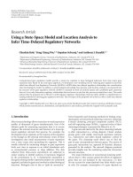
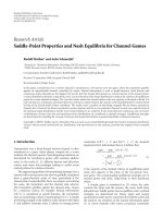
Figure 1: Annealed particle filter illustration for M=5. Initially the set contains many particles that represent very different poses and

therefore can fall into local maximum. On the last layer all the particles are close to the global maximum, and therefore they represent the
correct pose.
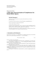
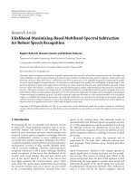
(a) (b)
Figure 2: (a) The 3D body model and (b) the samples drawn for
the weighting function calculation. In (b) the blue samples are used
to evaluate the edge matching, the cyan points are used to calculate
the foreground matching, the rectangles with the edges on the red
points are used to calculate the part-based body histogram.
smoothed version of it. The samples should be drawn from
the w
0
(y
n
, x) function, which might be peaky, and therefore
a large number of particles are needed to be used in order to
find the global maxima. Therefore, w
M
(y
n
, x) is designed to
be a very smoothed version of w
0
(y
n
, x). The usual method
to achieve this is by using w
m
(y
n
, x) = (w

0
(y
n
, x))
β
m
,where
1
= β
0
> ··· >β
M
and w
0
(y
n
, x) is equal to the origi-
nal weighting function. Therefore, each iteration of the an-
nealed particle filter algorithm consists of M steps, in each of
these the appropriate weighting function is used and a set of
pairs is constructed
{x
(i)
n,m
; π
(i)
n,m
}
N
p

i=1
. Tracking is described in
Algorithm 1.
Figure 1 shows the illustration of the 5-layered anneal-
ing particle filter. Initially the set contains many particles that
represent very different poses and therefore can fall into lo-
cal maximum. On the last layer all the particles are close to
the global maximum, and therefore they represent the cor-
rect pose.
4. GAUSSIAN FIELDS
The Gaussian process dynamical model (GPDM) (Lawrence
[3], Wang et al. [4]) represents a mapping from the latent
space to the data: y
= f (x), where x ∈ R
d
denotes a vector
in a d-dimensional latent space and y
∈ R
D
is a vector, that
represents the corresponding data in a D-dimensional space.
The model that is used to derive the GPDM is a mapping
with first-order Markov dynamics:
x
t
=

i
a
i

φ
i

x
t−1

+ n
x,t
,
y
t
=

j
b
j
ψ
j

x
t

+ n
y,t
,
(5)
where n
x,t
and n
y,t

are zero-mean Gaussian noise processes,
A
= [a
1
, a
2
, ]andB = [b
1
, b
2
, ] are weights, and φ
j
and
ψ
j
are basis functions.
4 EURASIP Journal on Advances in Signal Processing
00.20.40.60.81
0
500
1000
1500
2000
(a)
00.20.40.60.81
0
500
1000
1500
2000

(b)
00.20.40.60.81
0
500
1000
1500
2000
(c)
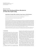
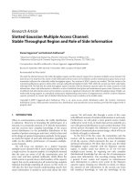
Figure 3: The reference histograms of the torso: (a) red, (b) green, and (c) blue colors of the reference selection.
−2 −10 12
−2
−1
0
1
(a)
−2
−1.5
−1
−0.5
0
0.5
1
1.5
2
−2
−1
0
1
2
−4

−2
0
2
(b)
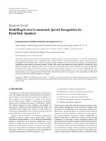
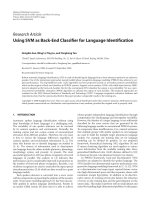
Figure 4: The latent space that is learned from different poses during the walking sequence. (a) The 2D space; (b) the 3D space. The brighter
pixels (a) correspond to more precise mapping.
For Bayesian perspective, A and B should be marginalized
out through model average with an isotropic Gaussian prior
on B in closed form to yield
P

Y | X,β

=
|
W|
N

(2π)
ND


K
y


D
e
−(1/2)tr(K
−1

y
YW
2
Y
T
)
,(6)
where W is a scaling diagonal matrix, Y is a matrix of training
vectors, X contains corresponding latent vectors, and K
y
is
the kernel matrix:

K
y

i,j
= β
1
e
−(β
2
/2)x
i
−x
j

+
δ
x

i
,x
j
β
3
,(7)
W is a scaling diagonal matrix. It is used to account for the
different variances in different data elements. The hyper pa-
rameter β
1
represents the scale of the output function, β
2
rep-
resents the inverse of the radial basis function (RBF) and β
−1
3
represents the variance of n
y,t
. For the dynamic mapping of
the latent coordinates X, the joint probability density over
the latent coordinate system and the dynamics weights A are
formed with an isotropic Gaussian prior over the A,itcanbe
shown (see Wang et al. [4]) that
P(X
| α) =
P

x
1



(2π)
(N−1)d


K
x


d
e
−(1/2)tr(K
−1
x
X
out
X
T
out
)
,(8)
where X
out
= [x
2
, , x
N
]
T
, K

x
is a kernel constructed
from [x
1
, , x
N−1
]
T
and x
1
has an isotropic Gaussian prior.
GPDM uses a “linear + RBF” kernel with parameter α
i
:

K
y

i,j
= α
1
e
−(α
2
/2)x
i
−x
j

+ α

3
x
T
i
x
j
+
δ
x
i
,x
j
α
4
. (9)
Following Wang et al. [4],
P(X,
α, β | Y) ∝ P(Y | X,β)P(X | α)P(α)P(β) (10)
the latent positions and hyper parameters are found by max-
imizing this distribution or minimizing the negative log pos-
terior:
Λ
=
d
2
ln


K
x



+
1
2
tr

K
−1
x
X
out
X
T
out

+

i
lnα
i
−Nln|W|
+
D
2
ln


K
y



+
1
2
tr

K
−1
y
YW
2
X
T

+

i
lnβ
i
.
(11)
5. GPAPF FILTERING
5.1. The model
In our work we use a model similar to the one proposed by
Deutscher et al. [5]withsomedifferences in the annealing
Leonid Raskin et al. 5
Used
X
Y

Z
(Frame 137)
(a)
Used
X
Y
Z
(Frame 138)
(b)
Used
X
Y
Z
(Frame 137)
(c)
Used
X
Y
Z
(Frame 138)
(d)
Figure 5: Losing and finding the tracked target despite the miss-tracking on the previous frame. (a) Frame 137, camera 1; (b) frame 138,
camera 1; (c) frame 137, camera 4; (d) frame 138, camera 4.
Initialization: {x
(i)
n,M
;1/N}
N
p
i=1

for each: frame n
for m
= M downto 0 do
1. Calculate the weights: π
(i)
n
= k (w
m
(y
n
, x
(i)
n,m
)p(x
(i)
n,m
| x
(i)
n,m
−1
)/q(x
(i)
n,m
| x
(i)
n,m
−1
, y
n
)), where

k
= (

N
p
i=1
(w
m
(y
n
| x
(i)
n,m
)p(x
(i)
n,m
| x
(i)
n,m
−1
)/q(x
(i)
n,m
| x
(i)
n,m
−1
, y
n
)))

−1
.
2. Draw N particles from the weighted set
{x
(i)
n,m
; π
(i)
n,m
}
N
p
i=1
with replacement and
with distribution p(x
= x
(i)
n,m
) = π
(i)
n,m
.
3. Calculate x
(i)
n,m−1
∼q(x
(i)
n,m−1
| x
(i)

n,m
, y
n
) = x
(i)
n,m
+ n
m
,wheren
m
is a Gaussian
noise n
m
N(0,P
m
).
end for
– The optimal configuration can be calculated using the following formula:
x
n
=

N
p
i=1
π
(i)
n,0
x
(i)

n,0
.
– The unweighted particle set for the next observation is produced using
x
(i)
n+1,M
= x
(i)
n,0
+ n
0
,wheren
0
is a Gaussian noise n
m
N(0,P
0
).
end for each
Algorithm 1: The annealed particle filter algorithm.
schedule and weighting function. The body model is defined
by a pair M
={L, Γ},whereL stands for the limbs lengths
and Γ for the angles between the limbs and the global loca-
tion of the body in 3D. The limbs parameters are constant,
and represent the actual size of the tracked person. The an-
gles represent the body pose and, therefore, are dynamic. The
state is a vector of dimensionality 29 : 3 DoF for the global 3D
location, 3 DoF for the global rotation, 4 DoF for each leg,
4DoFforthetorso,4DoFforeacharm,and3DoFforthe

head (see Figure 2). The whole tracking process estimates the
angles in such a way that the resulting body pose will match
the actual pose. This is done by maximizing the weighting
function which is explained next.
5.2. The weighting function
In order to evaluate how well the body pose matches the ac-
tual pose using the particle filter tracker we have to define
a weighting function w(Γ, Z), where Γ is the model’s con-
figuration (i.e., angles) and Z stands for visual content (the
captured images). The weighting function that we use is a
version of the one suggested by Deutscher and Reid [6]with
some modifications. We have experimented with 3 different
features: edges, foreground silhouette, and foreground his-
togram.
The first feature is the edge map. As Deutscher and Reid
[6] propose, this feature is the most important one, and pro-
vides a good outline for visible parts, such as arms and legs.
The other important property of this feature is that it is in-
variant to the color and lighting condition. The edge maps, in
which each pixel is assigned a value dependent on its proxim-
ity to an edge, are calculated for each image plane. Each part
is projected on the image plane and samples of the N
e
hy-
pothesized edges of human body model are drawn. A sum-
squared difference function is calculated for these samples:
Σ
e
(Γ, Z) =
1

N
cv
1
N
e
N
cv

i=1
N
e

j=1

1 − p
e
j

Γ, Z
i

2
, (12)
where N
cv
is a number of camera views, and Z
i
stands for the
image from the ith camera. The p
e

j
(Γ, Z
i
) are the edge maps.
Each part is projected on the image plane and samples of the
N
e
hypothesized edges are drawn.
However, the problem that occurs using this feature is
that the occluded body parts will produce no edges. Even the
visible parts, such as the arms, may not produce the edges,
6 EURASIP Journal on Advances in Signal Processing
Y
n
Y
n
Ω
n,N
Λ
n,N
Ω
n,M−1
Λ
n,M−1
ω
n,N
ω
n,M−1
···
Y

n
Y
n
Y
n+1
Ω
n,1
Λ
n,1
Ω
n,0
Λ
n,0
Ω
n+1,N
Λ
n+1,N
ω
n,1
ω
n+1,N
Figure 6: GPAPF with additional annealing layer graphical model. The black solid arrows represent the dependencies between state and the
visual data; the blue arrows represent the dependencies between the latent space and the data space; dashed magenta arrows represent the
dependencies between sequential annealing layers; the red arrows represent the dependencies of the additional annealing layer. The green
arrows represent the dependency between sequential frames.
0 20 40 60 80 100
Frame number
25
30
35

40
45
50
55
60
65
Prediction error
Figure 7: The errors GPAPF tracer with additional annealing layer
(blue circles) and without it (red crosses) for a walking sequence
captured at 30 fps.
because of the color similarity between the part and the body.
This will cause p
e
j
(Γ, Z
i
) to be close to zero and thus will
increase the squared difference function. Therefore, a good
pose which represents well the visual context may be omitted.
In order to overcome this problem for each combination of
image plane and body part, we calculate a coefficient which
indicates how well the part can be observed on this image.
For each sample point on the model’s edge we estimate the
probability being covered by another body part. Let N
i
be the
number of hypothesized edges that are drawn for the part i.
The total number of drawn sample points can be calculated
using N
e

=

N
bp
i=1
N
i
,whereN
bp
is the total number of body
parts in the model. The coefficient of part i for the image
plane j can be calculated as follows:
λ
i,j
=
1
N
i
N
i

k=1

1 − p
fg
k

Γ
i
, Z

j


2
, (13)
where Γ
i
is the model configuration for part i and p
fg
k
(Γ
i
, Z
j
)
is the value of the foreground pixel map of the sample k.If
a body part is occluded by another one, then the value of
p
fg
k
(Γ
i
, Z
j
) will be close to one and therefore the coefficient of
this part for the specific camera will be low. We propose us-
ing the following function instead of sum-squared difference
function as presented in (12):
Σ
e

(Γ, Z) =
1
N
cv
1
N
e
N
bp

i=1
N
cv

j=1
λ
i,j
Σ

Γ
i
, Z
j

, (14)
where
Σ

Γ
bp

, Z
cv

=
N
i

k=1

1 − p
e
k

Γ
bp
, Z
cv

2
. (15)
The second feature is the silhouette obtained by subtract-
ing the background from the image. The foreground pixel
map is calculated for each image plane with background pix-
els set to 0 and foreground set to 1 and sum-squared differ-
ence function is computed:
Σ
fg
(Γ, Z) =
1
N

cv
1
N
e
N
cv

i=1
N
e

j=1

1 − p
fg
j

Γ, Z
i

2
, (16)
where p
fg
j
(Γ, Z
i
) is the value is the foreground pixel map val-
ues at the sample points.
The third feature is the foreground histogram. The refer-

ence histogram is calculated for each body part. It can be a
grey level histogram or three separated histograms for color
images, as shown in Figure 3. Then, on each frame a nor-
malized histogram is calculated for a hypothesized body part
location and is compared to the referenced one. In order
to compare the histograms we have used the squared Bhat-
tacharya distance [30, 31], which provides a correlation mea-
sure between the model and the target candidates:
Σ
h
(Γ, Z) =
1
N
cv
1
N
bp
N
bp

i=1
N
cv

j=1

1 − ρ
part

Γ

i
, Z
j

, (17)
where
ρ
part

Γ
bp
, Z
cv

=
N
bins

i=1

p
ref
i

Γ
bp
, Z
cv

p

hyp
k

Γ
bp
, Z
cv

(18)
Leonid Raskin et al. 7
Used
X
Y
Z
(a)
Used
X
Y
Z
(b)
Used
X
Y
Z
(c)
Used
X
Y
Z
(d)

Figure 8: (a) and (b) GPAPF algorithm without the additional layer; (c) and (d) GPAPF algorithm with the additional layer.
Used
X
Y
Z
Frame 37
Used
X
Y
Z
Used
X
Y
Z
Used
X
Y
Z
(a)
Used
X
Y
Z
Frame 73
Used
X
Y
Z
Used
X

Y
Z
Used
Y
Z
(b)
Used
X
Y
Z
Frame 117
Used
X
Y
Z
Used
X
Y
Z
Used
X
Y
Z
(c)
Used
X
Y
Z
Frame 153
Used

X
Y
Z
Used
X
Y
Z
Used
X
Y
Z
(d)
Used
X
Y
Z
Frame 197
Used
X
Y
Z
Used
X
Y
Z
Used
X
Y
Z
(e)

Figure 9: Tracking results of annealed particle filter tracker and GPAPF tracker. Sample frames from the walking sequence. First row: GPAPF
tracker, first camera. Second row: GPAPF tracker, second camera. Third row: annealed particle filter tracker, first camera. Forth row: annealed
particle filter tracker, second camera.
and p
ref
i
(Γ
bp
, Z
cv
) is the value of bin i of the body part bp on
the view cv in the reference histogram, and the p
hyp
i
(Γ
bp
, Z
cv
)
is the value of the corresponding bin on the current frame
using the hypothesized body part location.
The main drawback of that feature is that it is sensitive
to changes in the lighting conditions. Therefore, the refer-
ence histogram has to be updated, using the weighted average
from the recent history.
In order to calculate the total weighting function the fea-
tures are combined together using the following formula:
w(Γ,Z)
= e
−(Σ

e
(Γ,Z)+Σ
fg
(Γ,Z)+Σ
h
(Γ,Z))
. (19)
As was stated above, the target of the tracking process is equal
to maximizing the weighting function.
5.3. GPAPF learning
The drawback in the particle filter tracker is that a high di-
mensionality of the state space causes an exponential increase
in the number of particles that are needed to be generated in
order to preserve the same density of particles. In our case,
the data dimension is 29D. In their work, Sigal et al. [7]
show that the annealed particle filter is capable of tracking
body parts with 125 particles using 60 fps video input. How-
ever, using a significantly lower frame rate (15 fps) causes the
tracker to produce bad results and eventually to lose the tar-
get.
The other problem of the annealed particle filter tracker
is that once a target is lost (i.e., the body pose was wrongly
estimated, which can happen for the fast and not smooth
movements) it is highly unlikely that the pose on the follow-
ing frames will be estimated correctly.
In order to reduce the dimension of the space we intro-
duce Gaussian process annealed particle filter (GPAPF). We
use a set of poses in order to create a low-dimensional la-
tent space. The latent space is generated by applying nonlin-
ear dimension reduction on the previously observed poses of

different motion types, such as walking, running, punching,
and kicking. We divide our state into two independent parts.
The first part contains the global 3D body rotation and trans-
lation parameters and is independent of the actual pose. The
8 EURASIP Journal on Advances in Signal Processing
0 50 100 150 200
Frame number
20
30
40
50
60
70
80
90
100
110
Prediction error
Figure 10: The errors of the annealed tracker (red crosses) and
GPAPF tracker (blue circles) for a walking sequence captured at
30 fps.
second part contains only information regarding the pose (26
DoF). We use Gaussian process dynamical model (GPDM) in
order to reduce the dimensionality of the second part and to
construct a latent space, as shown in Figure 4.GPDMisable
to capture properties of high-dimensional motion data bet-
ter than linear methods such as PCA. This method generates
a mapping function from the low-dimensional latent space
to the full data space. This space has a significantly lower di-
mensionality (we have experimented with 2D or 3D). Unlike

Urtasun et al. [28], whose latent state variables include trans-
lation and rotation information, our latent space includes
solely pose information and is therefore rotation and trans-
lation invariant. This allows using the sequences of the latent
coordinates in order to classify different motion types.
We use a 2-stage algorithm. In the first stage a set of new
particles is generated of in the latent space. Then we apply the
learned mapping function that transforms latent coordinates
to the data space. As a result, after adding the translation and
rotation information, we construct 31-dimensional vectors
that describe a valid data state which includes location and
pose information, in the data space. In order to estimate how
well the pose matches the images the likelihood function, as
described in the previous section, is calculated.
The main difficulty in this approach is that the latent
space is not uniformly distributed. Therefore, we use the dy-
namic model, as proposed by Wang et al. [4], in order to
achieve smoothed transitions between sequential poses in the
latent space. However, there are still some irregularities and
discontinuities. Moreover, while in a regular space the change
in the angles is independent on the actual angle value, in a
latent space this is not the case. Each pose has a certain prob-
ability to occur and thus the probability to be drawn as a
hypothesis should be dependent on it. For each particle we
can estimate the variance that can be used for generation of
the new ones. In Figure 4(a) the lighter pixels represent lower
variance, which depicts the regions of the latent space that
produce more likely poses.
Another advantage of this method is that the tracker is
capable of recovering after several frames, from poor esti-

mations. The reason for this is that particles generated in
the latent space are representing valid poses more authen-
tically. Furthermore, because of its low dimensionality, the
latent space can be covered with a relatively small number
of particles. Therefore, most of possible poses will be tested
with emphasis on the pose that is close to the one that was
retrieved in the previous frame. So if the pose was estimated
correctly, the tracker will be able to choose the most suitable
one from the tested poses. However, if the pose on the pre-
vious frame was miscalculated, the tracker will still consider
the poses that are quite different. As these poses are expected
to get higher value of the weighting function, the next lay-
ers of the annealing process will generate many particles us-
ing these different poses. As shown in Figure 5, the pose in
this way is likely to be estimated correctly, despite the miss-
tracking on the previous frame.
In addition the generated poses are, in most cases, nat-
ural. The large variance in the data space causes the genera-
tion of unnatural poses by the condensation or by annealed
particle filtering algorithms. In the introduced approach the
poses that are produced by the latent space that correspond
to points with low variance are usually natural as the whole
latent space is constructed based on learning from a set of
valid poses. The unnatural poses correspond to the points
with the large variance (black regions in Figure 4(a)) and,
therefore, it is highly unlikely that it will be generated. There-
fore, the effective number of the particles is higher, which en-
ables more accurate tracking.
As shown in Figure 4 the latent space is not continuous.
Two sequential poses may appear not too close in the latent

space; therefore, there is a minimal number of particles that
should be drawn in order to be able to perform the tracking.
The other drawback of this approach is that it requires
more calculation than the regular annealed particle filter due
to the transformation from the latent space into the data
space. However, as it is mentioned above, if the same number
of particles is used, the number of the effective poses is sig-
nificantly higher in the GPAPF then in the original annealed
particle filter. Therefore, we can reduce the number of the
particles for the GPAPF tracker, and by this compensate for
the additional calculations.
5.4. GPAPF algorithm
As we have explained before we are using a 2-stage algorithm.
The state consists of 2 statistically independent parts. The
first one describes the body 3D location: the rotation and
the translation (6 DoF). The second part describes the ac-
tual pose, that is, the latent coordinates of the corresponding
point in the Gaussian space (that was generated as we have
explained in Section 5.3). The second part usually has a very
smallDoF(aswasmentionedbeforewehaveexperimented
with 2- and 3-dimensional latent spaces). The first stage is the
generation of new particles. Then we apply the learned trans-
form function that transforms latent coordinates to the data
space (25 DoF). As the result, after adding the translation and
rotation information, we construct a 31-dimensional vectors
Leonid Raskin et al. 9
Figure 11: Tracking results of annealed particle filter tracker and GPAPF tracker. Sample frames from the running, leg movements and
object lifting sequences.
that describe a valid data state, which includes location and
pose information, in the data space. Then the state is pro-

jected to the cameras in order to estimate how well it fits the
images.
SupposewehaveM annealing layers. The state is de-
fined as a pair Γ
={Λ, Ω},whereΛ is the location infor-
mation and Ω is the pose information. We also define ω
as a latent coordinates corresponding to the data vector Ω:
Ω
= ℘(ω), where ℘ is the mapping function learned by the
GPDM. Λ
n,m
, Ω
n,m
,andω
n,m
are the location, pose vector,
and corresponding latent coordinates on the frame n and an-
nealing layer m.Foreach1
≤ m ≤ M − 1, Λ
n,m
and ω
n,m
are generated by adding multidimensional Gaussian random
variable to Λ
n,m+1
and ω
n,m+1
,respectively.ThenΩ
n,m
is cal-

culated using ω
n,m
. Full body state Γ
n,m
={Λ
n,m
, Ω
n,m
} is
projected to the cameras and the likelihood π
n,m
is calcu-
lated using likelihood function as explained in Section 5.2
(see Algorithm 2).
In the original annealed particle filter algorithm, the op-
timal configuration is achieved by calculating the weighted
average of the particles in the last layer. However, as the la-
tent space is not an Euclidian one, applying this method on
ω will produce poor results. The other method is choosing
the particle with the highest likelihood as the optimal config-
uration ω
n
= ω
(i
max
)
n,0
,wherei
max
= arg min

i
(π
(i)
n,m
). However,
this is an unstable way to calculate the optimal pose, as in
order to ensure that there exists a particle which represents
the correct pose, we have to use a large number of particles.
Therefore, we propose to calculate the optimal configuration
in the data space and then project it back to the latent space.
At the first stage we apply the
℘ on all the particles to generate
vectors in the data space. Then in the data space we calculate
the average on these vectors and project it back to the latent
space. It can be written as ω
n
= ℘
−1
(

N
i
=1
π
(i)
n,0
℘(ω
(i)
n,0
)).

5.5. Towards more precise tracking
The problem with such a 2-stage approach is that Gaussian
field is not capable to describe all possible posses. As we have
mentioned above, this approach resembles using probabilis-
tic PCA in order to reduce the data dimensionality. However,
for tracking issues we are interested to get the pose estimation
as close as possible to the actual one. Therefore, we add an
additional annealing layer as the last step. This stage consists
from only one stage. We use data states, which were generated
on the previous 2 staged annealing layer, described in previ-
ous section, in order to generate data states for the next layer.
This is done with very low variances in all the dimensions,
which practically are equal for all actions, as the purpose of
this layer is to make only the slight changes in the final es-
timated pose. Thus it does not depend on the actual frame
rate, contrary to original annealing particle tracker, where if
the frame rate is changed one need to update the model pa-
rameters (the variances for each layer).
ThefinalschemeofeachstepisshowninFigure 6 and
described in Algorithm 3. Suppose we have M annealing lay-
ers, as explained in Section 5.4, then we add one more single-
staged layer. In this last layer the Ω
n,0
is calculated using only
the Ω
n,1
without calculating the ω
n,0
. We should also pay at-
tention that the last layer has no influence on the quality of

tracking in the following frames, as ω
n,1
is used for the ini-
tialization of the next layer. Figure 7 shows the difference be-
tween the version without the additional annealing layer and
the results after adding it. We have used 5 2-staged annealing
layers in both cases. For the second tracker, we have added
additional single staged layer. In Figure 7 the error graphs are
shown that were produced by two trackers. The error was cal-
culated, based on comparison of the trackers output and the
result of the MoCap system. The comparison was suggested
by Sigal et al. [7]. This is done by calculating the 3D distance
between the locations of the different joints that is estimated
by the MoCap system and by the trackers results. The joints
that are used are hips, knees, and so forth. The distances are
summed and multiplied by the weight of the corresponding
particle. Then the sum of the all weighted distances is calcu-
lated, which is used as an error measurement. We can see that
the error, produced by GPAPF tracker without the additional
layer (blue circles on the graph), is lower than the one pro-
duced by the original GPAPF algorithm with the additional
annealing layer red crosses on the graph) for the walking se-
quence taken at 30 fps. We can notice that the error is lower
when we add the layer. However, as we have expected, the im-
provement is not dramatic. This is explained by the fact that
the difference between the estimated pose using only the la-
tent space annealing and the actual pose is not very big. That
10 EURASIP Journal on Advances in Signal Processing
Initialization: {Λ
(i)

n,M
; ω
(i)
n,M
;1/N}
N
p
i=1
for each: frame n
for m
= M downto 1 do
1. Calculate Ω
(i)
n,M
= ℘(ω
(i)
n,M
) applying the prelearned by GPDM mapping
function
℘ on the set of particles {ω
(i)
n,M
}
N
p
i=1
.
2. Calculate the weights of each particle:
π
(i)

n
= k(w
m
(y
n
, Λ
(i)
n,m
, ω
(i)
n,m
)p(Λ
(i)
n,m
, ω
(i)
n,m
| Λ
(i)
n,m
−1
, ω
(i)
n,m
−1
)/q(Λ
(i)
n,m
, ω
(i)

n,m
| Λ
(i)
n,m
, ω
(i)
n,m
−1
, y
n
)),
where k
= (

N
p
i=1
(w
m
(y
n
, Λ
(i)
n,m
, ω
(i)
n,m
)p(Λ
(i)
n,m

, ω
(i)
n,m
| Λ
(i)
n,m
−1
, ω
(i)
n,m
−1
)/q(Λ
(i)
n,m
, ω
(i)
n,m
| Λ
(i)
n,m
, ω
(i)
n,m
−1
, y
n
)))
−1
.Nowthe
weighted set is constructed, which will be used to draw particles for the next layer.

3. Draw N particles from the weighted set
{Λ
(i)
n,m
; ω
(i)
n,m
; π
(i)
n,m
}
N
p
i=1
with
replacement and with distribution p(Λ
= Λ
(i)
n,m
, ω = ω
(i)
n,m
) = π
(i)
n,m
.
4. Calculate
{Λ
(i)
n,m

−1
; ω
(i)
n,m
−1
}∼q(Λ
(i)
n,m
−1
; ω
(i)
n,m
−1
| Λ
(i)
n,m
; ω
(i)
n,m
, y
n
), which can
be rewritten as Λ
(i)
n,m
−1
∼q(Λ
(i)
n,m
−1

| Λ
(i)
n,m
, y
n
) = Λ
(i)
n,m
+ n
Λ
m
and
ω
(i)
n,m
−1
∼q(ω
(i)
n,m
−1
| ω
(i)
n,m
, y
n
) = ω
(i)
n,m
+ n
ω

m
,wheren
Λ
m
and n
ω
m
are multivariate Gaussian
random variables.
end for
– The optimal configuration can be calculated using the following formula:
Λ
n
=

N
p
i=1
π
(i)
n,1
Λ
(i)
n,1
and ω
n
= ω
(i
max
)

n,1
,wherei
max
= arg min
i
(π
(i)
n,1
).
– The unweighted particle set for the next observation is produced using
Λ
(i)
n+1,M
= Λ
(i)
n,1
+ n
Λ
1
and ω
(i)
n+1,M
= ω
(i)
n,1
+ n
ω
1
,wheren
Λ

1
and n
ω
1
are multivariate Gaussian
random variables.
end for each
Algorithm 2: The GPAPF algorithm.
suggests that the latent space accurately represents the data
space.
We can also notice that the improved GPAPF has less
peaks on the error graph. The peaks stem from the fact that
the argmax function, that has been used to find the opti-
mal configuration, is very sensitive to the location of the
best fitting particle. In the improved version, we calculate
weighted average of all the particles. As we have seen from
our experiments, there are often many particles with the
weight close to the optimal. Therefore, the result is less sensi-
tive to the location of some particular particle. It depends on
the whole set of them.
We have also tried to use the results, produced by the
additional layer, in order to initialize the state in the next
time step. This was done by applying the inverse function
℘
−1
, suggested by Lawrence and Candela [32], on the par-
ticles that were generated in previous annealing layer. How-
ever, this approach did not produce any valuable improve-
ment in the tracking results. As the inverse function is com-
putationally heavy it caused significant increase in the calcu-

lation time. Therefore, we decided not to experiment with it
further.
6. RESULTS
We have tested GPAPF tracking algorithm using HumanEva
dataset [33]. The sequences contain different activities, such
as walking, boxing, and so forth, which were captured by 7
cameras; however, we have used only 4 inputs in our evalua-
tion. The sequences were captured using the MoCap system
that provides the correct 3D locations of the body parts for
evaluation of the results and comparison to other tracking
algorithms.
Thefirstsequencethatwehaveusedwasawalkonacir-
cle. The video was captured at frame rate 120 fps. We have
tested the annealed particle filter-based body tracker, imple-
mented by A. Balan, and compared the results with the ones
produced by the GPAPF tracker. The error was calculated,
based on comparison of the tracker’s output and the result
of the MoCap system, using average distance between 3D
joints location, as explained in Section 5.4. Figure 10 shows
the error graphs, produced by GPAPF tracker (blue circles)
and by the annealed particle filter (red crosses) for the walk-
ing sequence taken at 30 fps. As can be seen, the GPAPF
tracker produces more accurate estimation of the body loca-
tion. Same results were achieved for 15 fps. Figure 9 presents
sample images with the actual pose estimation for this se-
quence. The poses are projected to the first and second cam-
eras. The first 2 rows show the results of the GPAPF tracker.
The third and forth rows show the results of the annealed
particle filter.
We have experimented with 100 particles up to 2000 par-

ticles. For the 100 particles per layer using 5 annealed layers,
the computational cost was 30 seconds per frame. Using the
same number of particles and layers in the annealed parti-
cle filter algorithm takes 20 seconds per frame. However, the
annealed particle filter algorithm was not capable of tracking
the body pose with such a low number of particles for 30 fps
and 15 fps videos. Therefore, we had to increase the number
of particles used in the annealed particle filter to 500.
We have also tried to compare our results to the re-
sults of condensation algorithm. However, the results of the
Leonid Raskin et al. 11
Initialization: {Λ
(i)
n,M
; ω
(i)
n,M
;1/N}
N
p
i=1
for each: frame n
for m
= M downto 1 do
1. Calculate Ω
(i)
n,M
= ℘(ω
(i)
n,M

) applying the prelearned by GPDM mapping
function
℘ on the set of particles {ω
(i)
n,M
}
N
p
i=1
.
2. Calculate the weights of each particle:
π
(i)
n
= k(w
m
(y
n
, Λ
(i)
n,m
, ω
(i)
n,m
)p(Λ
(i)
n,m
, ω
(i)
n,m

| Λ
(i)
n,m
−1
, ω
(i)
n,m
−1
)/q(Λ
(i)
n,m
, ω
(i)
n,m
| Λ
(i)
n,m
, ω
(i)
n,m
−1
, y
n
)),
where k
= (

N
p
i=1

(w
m
(y
n
, Λ
(i)
n,m
, ω
(i)
n,m
)p(Λ
(i)
n,m
, ω
(i)
n,m
| Λ
(i)
n,m−1
, ω
(i)
n,m−1
)/q(Λ
(i)
n,m
, ω
(i)
n,m
| Λ
(i)

n,m
, ω
(i)
n,m−1
, y
n
)))
−1
.
3. Draw N particles from the weighted set
{Λ
(i)
n,m
; ω
(i)
n,m
; π
(i)
n,m
}
N
p
i=1
with
replacement and with distribution p(Λ
= Λ
(i)
n,m
, ω = ω
(i)

n,m
) = π
(i)
n,m
.
4. Calculate
{Λ
(i)
n,m
−1
; ω
(i)
n,m
−1
}∼q(Λ
(i)
n,m
−1
; ω
(i)
n,m
−1
| Λ
(i)
n,m
; ω
(i)
n,m
, y
n

), which can
be rewritten as Λ
(i)
n,m
−1
∼q(Λ
(i)
n,m
−1
| Λ
(i)
n,m
, y
n
) = Λ
(i)
n,m
+ n
Λ
m
and
ω
(i)
n,m
−1
∼q(ω
(i)
n,m
−1
| ω

(i)
n,m
, y
n
) = ω
(i)
n,m
+ n
ω
m
,wheren
Λ
m
and n
ω
m
are multivariate Gaussian
random variables.
end for
– The optimal configuration can be calculated by the following steps:
1. Calculate
{Λ
(i)
n,m
−1
; Ω
(i)
n,m
−1
}∼q(Λ

(i)
n,m
−1
; Ω
(i)
n,m
−1
| Λ
(i)
n,m
; Ω
(i)
n,m
, y
n
), which can
be rewritten as Λ
(i)
n,m
−1
∼q(Λ
(i)
n,m
−1
| Λ
(i)
n,m
, y
n
) = Λ

(i)
n,m
+ n
Λ
m
and
Ω
(i)
n,m
−1
∼q(Ω
(i)
n,m
−1
| Ω
(i)
n,m
, y
n
) = q(Ω
(i)
n,m
−1
|
℘
(Ω
(i)
n,m
), y
n

) = ℘(Ω
(i)
n,m
)+n
Ω
m
,wheren
Λ
m
and n
Ω
m
are multivariate Gaussian random variables.
2. Draw N particles from the weighted set
{Λ
(i)
n,m
; Ω
(i)
n,m
; π
(i)
n,m
}
N
p
i=1
with distribution
p(Λ
= Λ

(i)
n,m
, Ω = Ω
(i)
n,m
) = π
(i)
n,m
. Calculate the weight of each particle.
3. The optimal configuration is Λ
n
=

N
p
i=1
π
(i)
n,0
Λ
(i)
n,0
and Ω
n
=

N
p
i=1
π

(i)
n,0
Ω
(i)
n,0
.
– The unweighted particle set for the next observation is produced using
Λ
(i)
n+1,M
= Λ
(i)
n,1
+ n
Λ
0
and ω
(i)
n+1,M
= ω
(i)
n,1
+ n
ω
0
,wheren
Λ
0
and n
ω

0
are multivariate Gaussian
random variables.
end for each
Algorithm 3: The GPAPF algorithm with the additional layer.
condensation algorithm were either very poor or a very large
number of particles needed to be used, which made this al-
gorithm computationally not effective. Therefore, we do not
show the results of this comparison.
The second sequence was captured in our lab. On that
sequence we have filmed similar behavior, produced by a
different actor. The frame rate was 15 fps. In case of walk-
ing, the learning was done on the first sequence data. The
GPAPF tracker was able to track the person and produced
results similar to the ones, which were produced for the orig-
inal sequence.
We have also experimented with sequences containing
different behavior, like leg movements, object lifting, clap-
ping, and boxing. We have manually marked some of the
sequences in order to produce the needed training sets
for GPDM. After the learning we have run the validation
on the other sequences containing same behavior. As it
is shown in the Figure 11, the tracker successfully tracked
these sequences. We have experimented with 100 going
up to 2000 particles. For the 100 particles, the computa-
tional cost was 30 seconds per frame. The results that are
shown in the videos are done with 500 particles (2.5 min-
utes per frame). The code that we are using is written in
Matlab with no optimization packages. Therefore, the com-
putational cost can be significantly reduced if moved to

Clibraries.
7. CONCLUSION AND FUTURE WORK
We have presented an approach that uses GPDM in order
to reduce the dimensionality and in this way to improve the
ability of the annealed particle filter tracker to track the ob-
ject even in a high-dimensional space. We have also shown
that using GPDM can increase the ability to recover from
temporal target loss. We have also presented a method to ap-
proximate the possibility of self occlusion and we have sug-
gested a way to adjust the weighed function for such cases,
in order to be able to produce more accurate evaluation of a
pose.
The main problem is that the learning and tracking are
done for a specific action. The ability of the tracker to use a
latent space in order to track a different motion type has not
been shown yet. A possible approach is to construct a com-
mon latent space for the poses from different actions. The
difficulty with such approach may be the presence of a large
number of gaps between the consecutive poses. In the future
we plan to extend the approach in order to be able to track
different activities, using the same learned data.
The other challenging task is to track two or more people
simultaneously. The main problem here is that in this case
there is high possibility of occlusion. Furthermore, while for
a single person each body part can be seen from at least one
camera that is not the case for the crowded scenes.
12 EURASIP Journal on Advances in Signal Processing
REFERENCES
[1] L. Raskin, E. Rivlin, and M. Rudzsky, “3D human tracking
with gaussian process annealed particle filter,” in Proceedings

of the 2nd International Conference on Computer Vision Theory
and Applications (VISAPP ’07), vol. 2, pp. 459–465, Barcelona,
Spain, March 2007.
[2] L. Raskin, M. Rudzsky, and E. Rivlin, “GPAPF: a combined ap-
proach for 3D body part tracking,” in Proceedings of the 5th In-
ternational Conference on Computer Vision Systems (ICVS ’07),
Bielefeld University, Germany, March 2007.
[3] N. D. Lawrence, “Gaussian process models for visualisation
of high dimensional data,” in Advances in Neural Information
Processing Systems (NIPS), vol. 16, pp. 329–336, 2004.
[4] J. Wang, D. J. Fleet, and A. Hetzmann, “Gaussian process dy-
namical models,” in Proceeding of the 19th Annual Confer-
ence on Neural Information Processing Systems (NIPS ’05),pp.
1441–1448, Vancouver, BC, Canada, December 2005.
[5] J. Deutscher, A. Blake, and I. Reid, “Articulated body motion
capture by annealed particle filtering,” in Proceedings of the
IEEE Conference on Computer Vision and Pattern Recognition
(CVPR ’00), vol. 2, pp. 126–133, Hilton Head Island, SC, USA,
June 2000.
[6] J. Deutscher and I. Reid, “Articulated body motion capture by
stochastic search,” International Journal of Computer Vision,
vol. 61, no. 2, pp. 185–205, 2005.
[7] A. O. B
˘
alan, L. Sigal, and M. J. Black, “A quantitative evalua-
tion of video-based 3D person tracking,” in Proceedings of the
2nd Joint IEEE International Workshop on Visual Surveillance
and Performance Evaluation of Tracking and Surve illance (VS-
PETS ’05), pp. 349–356, Beijing, China, October 2005.
[8] Y. Song, X. Feng, and P. Perona, “Towards detection of human

motion,” in Proceedings of the IEEE Conference on Computer
Vision and Pattern Recognition (CVPR ’00), vol. 1, pp. 810–
817, Hilton Head Island, SC, USA, June 2000.
[9] S. Ioffe and D. Forsyth, “Human tracking with mixtures of
trees,” in Proceedings of the 8th IEEE International Conference
on Computer Vision (ICCV ’01), vol. 1, pp. 690–695, Vancou-
ver, BC, Canada, July 2001.
[10] G. Mori and J. Malik , “Estimating human body configura-
tions using shape context matching,” in Proceedings of the 7th
European Conference on Computer Vision (ECCV ’02), vol. 3,
pp. 134–141, Copenhagen, Denmark, May 2002.
[11] H. Sidenbladh, M. J. Black, and D. J. Fleet, “Stochastic track-
ing of 3D human figures using 2D image motion,” in Pro-
ceedings of the 6th European Conference on Computer Vision
(ECCV ’00), vol. 2, pp. 702–718, Dublin, Ireland, June-July
2000.
[12] A. J. Davison, J. Deutscher, and I. D. Reid, “Markerless mo-
tion capture of complex full-body movement for character an-
imation,” in Proceedings of the Eurographic Workshop on Com-
puter Animation and Simulation, pp. 3–14, Manchester, UK,
September 2001.
[13] A. Agarwal and B. Triggs, “Learning to track 3D human mo-
tion from silhouettes,” in Proceedings of the 21st International
Conference on Machine Learning (ICML ’04), pp. 9–16, Banff,
Alberta, Canada, July 2004.
[14] A. Agarwal and B. Triggs, “3D human pose from silhouettes
by relevance vector regression,” in Proceedings of the IEEE
Computer Society Conference on Computer Vision and Pattern
Recognition (CVPR ’04), vol. 2, pp. 882–888, Washington, DC,
USA, June-July 2004.

[15] D. Ramanan and D. A. Forsyth, “Automatic annotation of ev-
eryday movements,” in Proceedings of the 15th Annual Confer-
ence on Neural Information Processing Systems (NIPS ’03),Van-
couver, BC, Canada, December 2003.
[16] M. Isard and J. MacCormick, “BraMBLe: a Bayesian multiple-
blob tracker,” in Proceedings of the 8th IEEE International Con-
ference on Computer Vision (ICCV ’01), vol. 2, pp. 34–41, Van-
couver, BC, Canada, July 2001.
[17] C. Bregler and J. Malik, “Tracking people with twists and ex-
ponential maps,” in Proceedings of the IEEE Computer Soci-
ety Conference on Computer Vision and Pattern Recognition
(CVPR ’98), pp. 8–15, Santa Barbara, Calif, USA, June 1998.
[18] H. Sidenbladh, M. J. Black, and L. Sigal, “Implicit probabilis-
tic models of human motion for synthesis and tracking,” in
Proceedings of 7th European Conference on Computer Vision
(ECCV ’02), vol. 1, pp. 784–800, Copenhaguen, Denmark,
May 2002.
[19] K. Mikolajczyk, K. Schmid, and A. Zisserman, “Human detec-
tion based on a probabilistic assembly of robust part detec-
tors,” in Proceedings of the 8th European Conference on Com-
puter Vision (ECCV ’04), vol. 1, pp. 69–82, Prague, Czech Re-
public, May 2003.
[20] K. Rohr, “Human movement analysis based on explicit motion
models,” in Motion-Based Recognition, chapter 8, pp. 171–198,
1997.
[21] D. Ormoneit, H. Sidenbladh, M. Black, and T. Hastie, “Learn-
ing and tracking cyclic human motion,” in Advances in Neural
Information Processing Systems 13, pp. 894–900, 2001.
[22] A. Elgammal and C S. Lee, “Inferring 3d body pose from sil-
houettes using activity manifold learning,” in Proceedings of

the IEEE Computer Society Conference on Computer Vision and
Pattern Recognition (CVPR ’04), vol. 2, pp. 681–688, Washing-
ton, DC, USA, June-July 2004.
[23] Q. Wang, G. Xu, and H. Ai, “Learning object intrinsic struc-
ture for robust visual tracking,” in Proceedings of the IEEE
Computer Society Conference on Computer Vision and Pattern
Recognition(CVPR ’03), vol. 2, pp. 227–233, Madison, Wis,
USA, June 2003.
[24] J. B. Tenenbaum, V. de Silva, and J. C. Langford, “A global ge-
ometric framework for nonlinear dimensionality reduction,”
Science, vol. 290, no. 5500, pp. 2319–2323, 2000.
[25] S. T. Roweis and L. K. Saul, “Nonlinear dimensionality reduc-
tion by locally linear embedding,” Science, vol. 290, no. 5500,
pp. 2323–2326, 2000.
[26] R. Urtasun and P. Fua, “3D human body tracking using de-
terministic temporal motion models,” in Proceedings of the 8th
European Conference on Computer Vision (ECCV ’04), vol. 3,
pp. 92–106, Prague, Czech Republic, May 2004.
[27] R. Urtasun, D. J. Fleet, A. Hertzmann, and P. Fua, “Priors
for people tracking from small training sets,” in Proceedings
of the 10th IEEE International Conference on Computer Vision
(ICCV ’05), vol. 1, pp. 403–410, Beijing, China, October 2005.
[28] R. Urtasun, D. J. Fleet, and P. Fua, “3D people tracking with
Gaussian process dynamical models,” in Proceedings of the
IEEE Computer Society Conference on Computer Vision and
Pattern Recognition (CVPR ’06), vol. 1, pp. 238–245, New York,
NY, USA, June 2006.
[29] M. Isard and A. Blake, “CONDENSATION—conditional den-
sity propagation for visual tracking,” International Journal of
Computer Vision, vol. 29, no. 1, pp. 5–28, 1998.

[30] D. Comaniciu, V. Ramesh, and P. Meer, “Kernel-based object
tracking,” IEEE Transactions on Pattern Analysis and Machine
Intelligence, vol. 25, no. 5, pp. 564–577, 2003.
Leonid Raskin et al. 13
[31] P. P
´
erez, C. Hue, J. Vermaak, and M. Gangnet, “Color-based
probabilistic tracking,” in Proceedings of 7th European Confer-
ence on Computer Vision (ECCV ’02), pp. 661–675, Copenh-
aguen, Denmark, May 2002.
[32] N. D. Lawrence and J. Qui
˜
nonero-Candela, “Local distance
preservation in the GP-LVM through back constraints,” in
Proceedings of the 23rd International Conference on Machine
Learning (ICML ’06), pp. 513–520, Pittsburgh, Pa, USA, June
2006.
[33] L. Sigal and M. J. Black, “Humaneva: cynchronized video and
motion capture dataset for evaluation of articulated human
motion,” Tech. Rep. CS-06-08, Brown University, Providence,
RI, USA, 2006.