Báo cáo hóa học: "Research Article Optimizing Training Set Construction for Video Semantic Classification" pdf

Hindawi Publishing Corporation
EURASIP Journal on Advances in Signal Processing
Volume 2008, Article ID 693731, 10 pages
doi:10.1155/2008/693731
Research Article
Optimizing Training Set Construction for Video
Semantic Classification
Jinhui Tang,
1
Xian-Sheng Hua,
2
Yan Song,
1
Tao Mei,
2
and Xiuqing Wu
1
1
Department of Electronic Engineering and Information Science, University of Science and Technology of China, Hefei 230027, China
2
Microsoft Research Asia, Beijing 100080, China
Correspondence should be addressed to Jinhui Tang,
Received 9 March 2007; Revised 14 September 2007; Accepted 12 November 2007
Recommended by Mark Kahrs
We exploit the criteria to optimize training set construction for the large-scale video semantic classification. Due to the large
gap between low-level features and higher-level semantics, as well as the high diversity of video data, it is difficult to represent
the prototypes of semantic concepts by a training set of limited size. In video semantic classification, most of the learning-based
approaches require a large training set to achieve good generalization capacity, in which large amounts of labor-intensive manual
labeling are ineluctable. However, it is observed that the generalization capacity of a classifier highly depends on the geometrical
distribution of the training data rather than the size. We argue that a training set which includes most temporal and spatial
distribution information of the whole data will achieve a good performance even if the size of training set is limited. In order to

capture the geometrical distribution characteristics of a given video collection, we propose four metrics for constructing/selecting
an optimal training set, including salience, temporal dispersiveness, spatial dispersiveness, and diversity.Furthermore,basedonthese
metrics, we propose a set of optimization rules to capture the most distribution information of the whole data using a training
set with a given size. Experimental results demonstrate these rules are effective for training set construction in video semantic
classification, and significantly outperform random training set selection.
Copyright © 2008 Jinhui Tang et al. This is an open access article distributed under the Creative Commons Attribution License,
which permits unrestricted use, distribution, and reproduction in any medium, provided the original work is properly cited.
1. INTRODUCTION
Video content analysis is an elementary step for mining the
semantic information in video collections, in which seman-
tic classification (or we may call it annotation) of video seg-
ments is essential for further analysis, as well as important for
enabling semantic-level video search. For human being, most
semantic concepts are clear and easy to identify, while due
to the large gap between semantics and low-level features,
the corresponding features generally are not well-separated
in feature space thus difficult to be identified by computer.
This is an open difficulty in computer vision and visual con-
tent analysis area.
Generally, learning-based video semantic classification
methods use statistical learning algorithms to model the se-
mantic concepts (generative learning) or the discriminations
among different concepts (discriminative learning). In [1],
hidden Markov model and dynamic programming are ap-
plied to play/break segmentation in soccer videos. Fan et al.
[2] classify semantic concepts for surgery education videos
by using Bayesian classifiers with an adaptive EM algorithm.
ZhongandChang[3] propose a unified framework for
scene detection and structure analysis by combining domain-
specific knowledge with supervised machine learning meth-

ods. However, most of these learning-based approaches re-
quire a large training set to achieve good generalization ca-
pacity, thus a great deal of labor-intensive manual labeling is
inevitable. On the other hand, semisupervised learning tech-
niques, which try to exploit the information embedded in
unlabeled data, are proposed to improve the performance.
In [4], cotraining is applied to video annotation based on a
careful split of visual features. Yan and Naphade [5] point out
the drawbacks of cotraining in video annotation, and pro-
pose an improved cotraining style algorithm named semisu-
pervised cross-feature learning. An structure-sensitive man-
ifold ranking method is proposed in [6] for video con-
cept detection, where the authors analyze the graph-based
semisupervised learning methods from the view of PDE-
based diffusion. Tang et al. [7] embed the temporal consis-
tency of video data into the graph-based SSL and propose
2 EURASIP Journal on Advances in Signal Processing
a temporally consistent Gaussian random field method for
video annotation. A method based on kernel density estima-
tion is proposed in [8] for video semantic detection, where
the authors show that this method has close relationship with
the graph based semisupervised learning. In addition, active
learning scheme is also an effective solution to this problem
[9, 10]. However, all these methods have paid little atten-
tion on the issue of the training set construction. Generally,
most of them adopt a random selection scheme to construct
the training set. In this paper, we argue that a better train-
ing set, though the size is very small, can be carefully con-
structed/selected with a good performance being simultane-
ously preserved.

It has been shown that the generalization capacity of a
classifier usually depends on the geometrical distribution of
the training data rather than the size [11]. Therefore, if the
selected training data can capture this kind of characteristic
of the entire video collection, the classification performance
will still be good enough even in the case that the size of
training set is much smaller than that of the whole dataset,
thus much manual labor for training data labeling will be
saved. In other words, according to the distribution analy-
sis of the video dataset, a “skeleton” of the prototypes of the
semantic concepts can be achieved in a training set with an
extremely limited number of samples.
Given a large video collection, it is possible to construct
a small-size but effective training set (to be labeled manu-
ally) by exploiting the temporal and spatial distribution of
the entire dataset. Typically, a semantic concept and its cor-
responding feature variations within the same video are rel-
atively smaller than those among different videos and the
concept drifting is gradual in most cases [12]. The cluster-
ing information can be extracted according to this observa-
tion. That is, based on visual similarity and temporal order,
the video shots can be preclustered in an over-segmentation
manner [4]. Each cluster can be represented by the cluster
center (or the shot closest to the cluster center in terms of
low-level features). This clustering process aims at making all
the samples within each cluster most likely associate with the
same semantic concept. As a result, the training set can be
constructed by selecting samples from these cluster centers.
Intuitively, we can take all the cluster centers as the train-
ing set. However, as clustering information is obtained in an

over-segmentation manner, typically the number of cluster
centers is very large. Therefore, much redundancy still exists
among these clusters and actually only a small part of them
is highly informative.
In this paper, we analyze the factors which can capture
the distribution characteristics of a given video collection,
and propose the following four metrics for the training set
construction, including salience, temporal dispersiveness, spa-
tial dispersiveness, and diversity. First, as the candidates for
constructing the training set are actually cluster centers, the
samples in this candidate set should have different potential
contributions to the training set as their corresponding clus-
ter sizes are different. Accordingly, we introduce salience,as
a potential contribution measure of each candidate sample.
Second, the samples in the training set should distribute dis-
persively in temporal order, as well as in the low-level feature
Video
database
Video shots
Features
Clusters
Data set
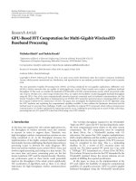
Figure 1: Preprocessing of video database.
space, thus more “prototypes” of the semantic concept can
be selected. Therefore, we introduce two measures, tempo-
ral dispersiveness and spatial dispersiveness,toreflecthowwell
the training set captures the distribution of the entire video
dataset in temporal order and the feature space, respectively.
Finally, in addition to temporal and spatial dispersiveness,
the selected samples need to be diversely distributed in the

feature space [13]. In this paper, the measure diversit y is de-
fined to capture this training set property.
According to the above analyses, a set of optimization
rules based on these metrics are further proposed to reduce
the redundancy in the set of cluster centers. A set of experi-
ments are conducted on a real-video dataset to show the ef-
fectiveness of these rules.
The rest of this paper is organized as follows. In Section 2,
representativeness metrics for training set construction are
presented. Section 3 discusses the optimization rules and
methods according to the representativeness metrics. Exper-
imental results are presented in Section 4, followed by con-
cluding remarks and future work in Section 5.
2. REPRESENTATIVENESS METRICS
In this section, we first describe the preprocessing step of
video database, including shot detection, feature extraction,
and preclustering. Then the four metrics including salience,
temporal dispersiveness, spatial disper siveness, and divers ity
are discussed in detail based on the preprocessing results.
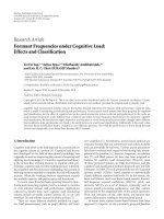
Figure 1 illustrates the flowchart of preprocessing the
video dataset. First, each video is segmented into shots ac-
cording to timestamp (for DVs) or visual similarity (for ana-
log videos). In the following process, each shot is represented
by a certain number of frames uniformly excerpted from the
shot. Shot is taken as the elementary unit for the semantic
classification in this paper, which is the basic annotation unit
most frequently applied in the literature.
All the shots in the video database are preclustered based
on their visual similarity measure and temporal order in an
over-segmentation manner, in which all the shots belonging

to a certain cluster mostly correspond to the same semantic
concept [4]. Then, in the process of classification, one clus-
ter is taken as one sample, instead of using one shot as an
individual sample, which can significantly reduce the num-
ber of shots that need to be labeled by users [14]. Yuan et al.
[15] also show that simply taking cluster centers for train-
ing works well with theoretical insight. Here our objective
Jinhui Tang et al. 3
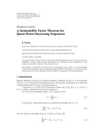
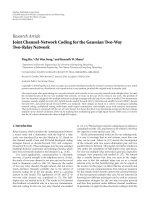
Figure 2: Exemplary thumbnails for the 4 different sematic classes. First row: landscape;secondrow:indoor; third row: cityscape;lastrow:
others.
is different from theirs. We aim to select a set of informa-
tive samples for the users to annotate and then the set is
used for training. Before the training set being constructed,
the labels are unknown, and they use the labels of the entire
dataset. Our objective is to reduce the manual work while
Yuan’s work focuses on reducing the number of support vec-
tors.
As aforementioned, the training set is constructed to
roughly represent the prototypes of the semantic concepts
to be modeled from the video collection. Here, we detail the
aforementioned four metrics to measure the representative-
ness of a training set. To clearly present our ideas, we define
the following notations at first.
Notation 1. The center (or representative shot) set of the
clusters is denoted by CntSet
={x
j
,1 ≤ j ≤ K(cl)},where
x
j

is the shot closest to the center of the jth cluster and K(cl)
is the total number of the clusters in the whole video dataset.
Notation 2. The training set consisted of the selected shots
from CntSet is denoted by TrnSet
={x
i
,1 ≤ i ≤ M},where
M is the size of training set that will be constructed. TrnSet
is a subset of CntSet.
Notation 3. The distance between two sample feature vectors
in the kernel mapped feature space is defined as dis(φ
i
, φ
j
):
dis

φ
i
, φ
j

=


φ

x
i


−
φ

x
j



=

φ
T
i
φ
i
− 2φ
T
i
φ
j
+ φ
T
j
φ
j
=

K

x

i
, x
i

−
2K

x
i
, x
j

+ K

x
j
, x
j

,
(1)
where φ
i
is the kernel mapping of the feature vector x
i
(we use
x to denote both the shot and its feature vector in this paper),
K is the kernel function. In our experiments, Gaussian kernel
is adopted for K.
Based on these notations, we introduce four metrics to

measure the effectiveness of a training set.
2.1. Salience metric
First, the effectiveness of samples (cluster centers) is different
from each other, that is, the sample corresponding to a large
cluster should be more “important” than the ones of small
clusters. In other words, such samples most likely represent
the salient prototypes of the semantic concepts. Therefore,
we define SAL as the salience metric of TrnSet as follows.
Metric 1. Salience:
SAL
=
1
K(cl)

x
i
∈TrnSet
Sal(x
i
), (2)
where Sal(x
i
) is the number of shots in the cluster corre-
sponding to the ith sample in TrnSet.
2.2. Temporal dispersiveness metric
Second, the samples to be selected should distribute disper-
sively through the temporal axis of the whole video dataset.
Thus more prototypes of the semantic concept can be pre-
served. This is from the observation that if the two salient
samples lie close to each other in temporal order, it may be-

long to the same concept with high probability. We define the
temporal distance between the sets CntSet and TrnSet as
Dis
T
=
1
K(cl)

x
j
∈CntSet
min
x
i
∈TrnSet


t

x
i

−
t

x
j




,(3)
where min
x
i
∈TrnSet
t(x
i
)−t(x
j
) is the temporal distance be-
tween x
j
and TrnSet, and t(x) is the normalized temporal or-
der of the sample x.Thetemporal dispersiveness is defined as
follows.
Metric 2. Temporal dispersiveness:
T
Disp =
1
Dis
T
=
K(cl)

x
j
∈CntSet
min
x
i

∈TrnSet


t

x
i

−
t

x
j



.
(4)
4 EURASIP Journal on Advances in Signal Processing
500450400350300250200150100
The number of selected samples
Random selection
Selection using salience
0.25
0.3
0.35
0.4
0.45
0.5
The error rate of classification

(a)
500450400350300250200150100
The number of selected samples
Random selection
Selection using temporal spersiveness only
Selection using temporal spersiveness with salience
0.1
0.15
0.2
0.25
0.3
0.35
0.4
0.45
The error rate of classification
(b)
500450400350300250200150100
The number of selected samples
Random selection
Selection using spatial dispersiveness only
Selection using spatial dispersiveness with salience
0.1
0.15
0.2
0.25
0.3
0.35
0.4
0.45
The error rate of classification

(c)
500450400350300250200150100
The number of selected samples
Random selection
Selection using diversity only
Selection using diversity and salience
0.2
0.25
0.3
0.35
0.4
The error rate of classification
(d)
500450400350300250200150100
The number of selected samples
Random selection
Selection using temporal spersiveness only
Selection using spatial spersiveness only
Selection using diversity only
Selection using Rule all
0.1
0.15
0.2
0.25
0.3
0.35
0.4
0.45
The error rate of classification
(e)

500450400350300250200150100
The number of selected samples
Using temporal spersiveness and salience
Using spatial spersiveness and salience
Using diversity and salience
Using Rule all
0.12
0.14
0.16
0.18
0.2
0.22
0.24
0.26
0.28
0.3
The error rate of classification
(f)
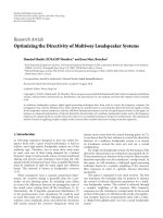
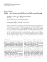
Figure 3: Comparisons of the experimental results in a transductive manner.
Jinhui Tang et al. 5
400350300250200150100
The number of selected samples
Random
Salience
Diversity
Spatial dispersiveness
Temporal dispersiveness
Salience + diversity
Salience + spatial disversiveness
Salience + temporal disversiveness

Rule-all
0.2
0.25
0.3
0.35
0.4
0.45
0.5
The error rate of classification
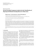
Figure 4: Comparisons of the experimental results after data sepa-
ration.
In order to assure that the TrnSet can capture most tem-
poral distribution information of the CntSet, it is necessary
to minimize the Dis
T
, which is equivalent to the maximiza-
tion of T
Disp. Thus, for each sample in CntSet, there should
be a sample in TrnSet close to it in temporal order. Given the
size of the TrnSet, maximizing T
Disp can mostly disperse
the samples in TrnSet in temporal order.
2.3. Spatial dispersiveness metric
Third, similar to the aforementioned temporal dispersive-
ness, the samples to be selected should distribute dispersively
through the whole kernel mapped feature space. This is from
the observation that if the two salient samples lie close to each
other in the feature space, it may belong to the same concept
with high probability. We define the spatial distance Dis
S

be-
tween the sets CntSet and TrnSet as
Dis
S
=
1
K(cl)

x
j
∈CntSet
min
x
i
∈TrnSet


φ

x
i

− φ

x
j



,(5)

where min
x
i
∈TrnSet
φ(x
i
) − φ(x
j
) is the spatial distance be-
tween x
j
and TrnSet. Then we define spatial dispe rsiveness as
follows.
Metric 3. Spatial dispersiveness:
S
Disp =
1
Dis
S
=
K(cl)

x
j
∈CntSet
min
x
i
∈TrnSet



φ

x
i

−
φ

x
j



,
(6)
where φ(x) is the kernel mapping of x. TrnSet can capture the
most spatial distribution characteristics of CntSet through
maximizing S
Disp. It corresponds to minimizing Dis
S
, that
is, the samples in CntSet have a minimal average distance to
TrnSet in the kernel mapped space. Thus, for each sample
x
j
in CntSet, there should be a sample in TrnSet close to it.
Given the size of TrnSet, maximization of S
Disp can mostly
disperse the samples in TrnSet in the mapped feature space.

2.4. Diversity metric
Gohetal.[13] have pointed out that the selected samples
need to be diversified in image retrieval application, and de-
fined the measure angle diversity to choose the sample with
the maximal angle (less than 90
◦
) to the current selected sam-
ple set. That is, the selected sample should be “almost or-
thogonal” to current selected sample set. However, their def-
inition of the angle between the unlabeled instance x
i
to the
current sample set S is the maximal angle from instance x
i
to
any instance x
j
in set S. This definition just ensures that the
chosen instances can be almost orthogonal to one sample in
current set, but not almost orthogonal to the set. We intro-
duce feature vector selection (FVS) method to handle this
problem. FVS method is proposed in [16] to find an approx-
imate basis of the whole dataset to reduce feature dimension.
Here we employ it to find the almost orthogonal sample set
in CntSet. FVS is similar to the kernel principal component
analysis (KPCA) while FVS selects the existed sample vectors
as the basis, and the KPCA uses the first k eigenvectors as the
basis. The authors of [16] show that in some special cases the
FVS-PCA is equivalent to KPCA.
As aforementioned, the samples in TrnSet are denoted as

{x
i
,1≤ i ≤ M},whereM is the size of TrnSet. Given a well-
selected TrnSet, each sample x
j
in CntSet could be approxi-
mated by the linear combination of samples in TrnSet in the
kernel mapped space. The normalized Euclidean distance δ
j
is defined to measure the fitness between φ(x
j
)and

φ(x
j
)as
follows:
δ
j
=


φ

x
j

−

φ


x
j



2


φ

x
j



2
,(7)
δ
j
is a similarity measure between the original vector φ(x
j
)
and the reconstructed vector

φ(x
j
) =

x

i
∈TrnSet
α
ji
φ(x
i
). The
smaller δ
j
is, the better x
j
can be approximated by TrnSet.
Consequently, the metric diversity can be defined as follows.
Metric 4. Diversity:
Divers
= 1 −
1
K(cl)

x
j
∈CntSet
δ
j
= 1 −
1
K(cl)

x
j

∈CntSet


φ

x
j

−

x
i
∈TrnSet
α
ji
φ

x
i



2


φ

x
j




2
,
(8)
where a
ij
are weights of the combination. This metric
demonstrates how the TrnSet can capture the diversity of
CntSet. Given the size of TrnSet, maximization of Divers can
6 EURASIP Journal on Advances in Signal Processing
lead the samples in TrnSet to be almost orthogonal to each
other. It is worth noting that the aim of spatial dispersive-
ness is to distribute the selected samples in the feature space
with maximal average distance under L1 norm. It is similar
to minimize the reconstruction error with the only closest
sample under L1 norm. The aim of diversity is to minimize
the linear reconstruction error under the L2 norm. They are
similar but have difference.
3. OPTIMIZATION RULES
As aforementioned, four metrics have been defined to mea-
sure the representativeness of TrnSet. According to these
metrics, the following rules are further proposed to construct
an optimal training set with a given size.
Rule 1. Maximizing salience:
TrnSet
∗
= argmax
TrnSet⊂CntSet
{SAL | #(TrnSet) = M},(9)

where #(TrnSet) is the number of samples in TrnSet, M is a
given number.
Theconstructingprocedurebasedonthisrulecanbede-
scribed as shown in Algorithm 1.
Rule 2. Maximizing temporal dispersiveness:
TrnSet
∗
= arg max
TrnSet⊂CntSet

T Disp | #(TrnSet) = M

. (10)
This rule is equal to minimize Dis
T
, and the training set con-
struction procedure is illustrated in Algorithm 2.
Rule 3. Maximizing spatial dispersiveness:
TrnSet
∗
= arg max
Tr nS et ⊂CntSet

S Disp | #(TrnSet) = M

. (11)
This rule is equal to minimize Dis
S
, and the procedure can
be accomplished similar to Rule 2, just needs to change the

temporal distance dt
mn
to the spatial distance dis(φ
m
, φ
n
) =

φ(x
m
) − φ(x
n
).
Rule 4. Maximization of diversity:
TrnSet
∗
= argmax
TrnSet⊂CntSet

Divers | #(TrnSet) = M

. (12)
So the target is to find a set (TrnSet) of feature vectors (FVs)
[16] with the fixed size which minimize

x
j
∈CntSet



φ

x
j

−

x
i
∈Tr nS et
α
ji
φ

x
i



2


φ

x
j



2

. (13)
Ithasbeenprovenin[16] that the minimization of
δ
j
=


φ

x
j

−

φ

x
j



2


φ

x
j




2
(14)
for a given size M of FVs can be expressed with dot products
only:
min δ
j
= 1 −
K
T
Sj
K
−1
SS
K
Sj
k
jj
, (15)
where
K
SS
=

K

x
p
, x
q


1≤p,q≤M
(16)
is a square matrix of dot products of FVs, and
K
Sj
=

K

x
p
, x
j

1≤p≤M
(17)
is the vector of dot products between x
j
and the FVs.
Define the fitness for the sample x
j
by
J
S
j
=




φ

x
j



2


φ

x
j



2
=
K
T
Sj
K
−1
SS
K
Sj
k
jj
, (18)

which is a measure of the best fit case, where x
j
∈ CntSet,
x
i
∈ Tr nSe t a nd k
jj
= K(x
j
, x
j
). Then the objective becomes
to select a set TrnSet for a given size M to maximize the fitness
for the CntSet:
JS
=
1
K(cl)

x
j
∈CntSet
J
S
j
. (19)
Note that the maximum of (19)isoneandforx
i
∈
Tr nSe t, ( 15) is zero. Therefore, when #(TrnSet) increases, we

only need to explore (K(l)
− #(TrnSet)) remaining vectors to
evaluate the maximization of JS.
The process is iterative, which consists of a set of sequen-
tial forward selection operations: at the first iteration, we
look for the sample that gives the maximum JS.Exceptfor
the first iteration, the algorithm uses the lowest fitness J
S
j
for
the current basis TrnSet to select the new FV while evaluat-
ing the JS. JS is monotonic since the new basis will recon-
struct all the samples at least as well as the previous basis did.
Algorithm 3 shows the detailed procedure.
Among the four metrics, salience is the property of each
sample, while the other three metrics are related to the cor-
relations between TrnSet and CntSet. Therefore, salience can
be combined into Rule 2–4 to improve the results.
Rule 1 + 2. Maximizing temporal dispersiveness with
salience.
1
We want the sample with high salience to have more
chance to be selected, so we can minimize

x
j
∈CntSet
min
x
i

∈Tr nS et


t

x
i

−
t

x
j



Sal

x
i

·Sal(x
j

(20)
subject to a fixed-size TrnSet. The training set construction
procedureofthisruleispresentedinAlgorithm 4.
1
The computation for optimizing Rule 1 + 2 is NP hard. For approxima-
tion, we remove the samples, which are not dispersive and salient ei-

ther, from the CntSet. Thus, the distance measure defined in step 2 of
Algorithm 4 is different from the definition in (20). The optimizations of
Rule 1 + 3 and Rule 1–3 also have this case.
Jinhui Tang et al. 7
1: Initialization: TrnSet :={}and #(TrnSet) = 0;
2: Obtain Sal(x
j
) for every sample x
j
in CntSet according to the cluster size;
3: While #(TrnSet) <M
Find the maximal element maxSal in vector [Sal(x
j
)]
1≤ j≤K(cl)
;
Add the sample corresponding to maxSal to TrnSet;
Remove this sample from CntSet;
#(TrnSet)
= #(TrnSet) + 1;
End While
4: Return TrnSet
Algorithm 1: Optimization of Rule 1.
1: Initialization: TrnSet: = CntSet and #(TrnSet) = K(cl);
2: In current TrnSet, compute the temporal distance between every two samples
dt
mn
=|t(x
m
) − t(x

n
)|, m=n. dt
mn
= inf when m = n. The temporal order is normalized;
3: While #(TrnSet) >M
Find the minimal element mindt in matrix [dt
mn
]
1≤m,n≤K(cl)
;
Remove the corresponding x
n
from TrnSet;
#(TrnSet)
= #(TrnSet) − 1;
Set dt
nk
= inf ; dt
kn
= inf ; k ∈{1,2, , K(cl)}
End While
4: Return TrnSet
Algorithm 2: Optimization of Rule 2.
Rule1+3. Maximizing spatial dispersiveness with salience.
Similar to Rule 1 + 2, we minimize

x
j
∈CntSet
min

x
i
∈Tr nS et
φ(x
i
) − φ(x
j
)
Sal(x
i
)·Sal(x
j
)
(21)
subject to a fixed-size TrnSet. This procedure is similar to
Rule 1 + 2.
Rule 1 + 4. Maximizing diversity accompanied with salience.
Consider the effect of salience, the objective becomes
finding a feature vector set (FVs) under the constraint of
fixed size to minimize

x
j
∈CntSet
φ(x
j
) −

x
i

∈Tr nS et
α
ji
φ(x
i
)
2
φ

x
j


2
·Sal

x
j

. (22)
Then we can select samples as the procedure in Algorithm 5.
Actually, finally, we want to use all these four metrics to
optimize TrnSet. A direct way is to maximize a linear combi-
nation of the four metrics, that is, to maximize
R
= α·SAL + β·T Disp
+ γ
·S Disp + (1 − α − β − γ)·Divers
(23)
subject to a fixed-size TrnSet. However, it is not easy to deter-

mine the three weights (which is our future work). Alterna-
tively, in this paper, we optimize the four metrics in a hierar-
chical way. That is, firstly we minimize

x
j
∈CntSet
min
x
i
∈Tr nS et
dis

φ
i
, φ
j

·dt

x
i
, x
j

Sal

x
i


·
Sal

x
j

(24)
to optimize the Metric 1–3 simultaneously (see Algorithm 6),
and then use Rule 1 + 4 to remove 10% redundancy. We call
this method Rule
all.
4. EXPERIMENTAL RESULTS
To evaluate the performance of our proposed algorithms on
real video dataset, we conduct several experiments on a home
video dataset which contains about 55 home videos with a
wide variety of contents, such as wedding, vacation, meeting,
party, and sports.
In the experiments, we classify the shots in the video
dataset into the following four semantic concepts: indoor,
landscape, cityscape, and others. The four semantic concepts
are mutually exclusive, that is, one sample just can belong to
one concept. After preprocessing of the video dataset includ-
ing shot detection, low-level feature extraction and preclus-
tering, about 7000 shots are obtained. These shots are further
clustered into about 1600 clusters in an over-segmentation
manner. Each shot is labeled as indoor, cityscape, landscape,
and others according to the definitions in TRECVID [17].
Some exemplary thumbnails of these concepts are shown in
Figure 2.
8 EURASIP Journal on Advances in Signal Processing

1: Initialization: TrnSet :={}and #(TrnSet) = 0;
2: For 1 <j<K(l)
Compute the J
S
j
using other K(l) − 1 samples as the basis;
End for
3: Find the largest J
S
j
and add the corresponding x
j
into TrnSet as the first sample;
4: While #(TrnSet) <M
For 1 <j<K(l)
Using current TrnSet as the basis, compute the J
S
j
;
End For
Find the smallest J
S
j
;
Add the corresponding x
j
into TrnSet;
#(TrnSet)
= #(TrnSet) + 1;
End While

5: Return TrnSet
Algorithm 3: Optimization of Rule 4.
1: Initialization: TrnSet = CntSet and #(TrnSet) = K(cl);
2: In current TrnSet, compute the following distance between every two samples
dt
mn
= Sal(x
m
)·Sal(x
n
)·dt(x
m
, x
n
), m=n. d
m,n
= inf when m = n. The temporal order is normalized;
3: While #(TrnSet) >M
Find the minimal element min
dt in matrix [dt
mn
]
1≤m,n≤K(cl)
;
Find the corresponding x
m
and x
n
;
If Sal(x

m
) ≥ Sal(x
n
)
Remove x
n
from TrnSet;
Set d
nk
= inf ; d
kn
= inf ; k ∈{1, 2, , K(cl)}
Else
Remove x
m
from TrnSet;
Set d
mk
= inf ; d
km
= inf ; k ∈{1, 2, , K(cl)}
End If
End While
4: Return TrnSet
Algorithm 4: Optimization of Rule 1 + 2.
1: Initialization: TrnSet :={}and #(TrnSet) = 0;
2: For 1 <j<K(l)
Compute the J
S
j

using other K(l) − 1 samples as the basis;
End for
3: Find the largest Sal(x
j
)J
S
j
and add the corresponding x
j
into TrnSet as the first sample;
4: While #(TrnSet) <M
For 1 <j<K(l)
Using current TerSet as the basis, compute the J
S
j
;
End For
Find the smallest Sal(x
j
)J
S
j
;
Add the corresponding x
j
into TrnSet;
#(TrnSet)
= #(TrnSet) + 1;
End While
5: Return TrnSet

Algorithm 5: Optimization of Rule 1 + 4.
Jinhui Tang et al. 9
1: Initialization: TrnSet = CntSet and #(TrnSet) = K(cl);
2: In current TrnSet, compute the following distance between every two samples
d
mn
= Sal(x
m
)·Sal(x
n
)·dis(φ
m
, φ
n
)·dt(x
m
, x
n
), m=n, d
mn
= inf when m = n ;
3: While #(TrnSet) >M
Find the minimal element min
d in matrix [d
mn
]
1≤m,n≤K(cl)
;
Find the corresponding x
m

and x
n
;
If Sal(x
m
) ≥ Sal(x
n
)
Remove x
n
from TrnSet;
Set d
nk
= inf ; d
kn
= inf ; k ∈{1, 2, , K(cl)}
Else
Remove x
m
from TrnSet;
Set d
mk
= inf ; d
km
= inf ; k ∈{1, 2, , K(cl)}
End If
End While
5: Return TrnSet
Algorithm 6: Optimization of Rule 1– 3.
The low-level features we used here has 90 dimensions,

consisting of a 36-D HSV color histogram, a 9D color mo-
ment, and a 45D blockwise edge distribution histogram.
Low-level features are normalized by Gaussian normaliza-
tion [18]. Each shot is represented by a certain number (i.e.,
10) of frames uniformly excerpted from the shot, and the
shot closest to the cluster center is taken as the sample to
form the dataset. So the dataset used in experiment has about
7000 samples, and each sample is represented as a 900D vec-
tor. The CntSet has about 1600 samples, and each sample is
also a 900D vector.
We conduct 5 experiments in transductive manner: when
the training set TrnSet is constructed, we train the SVM
model [19] to classify the samples in CntSet (here the pa-
rameters C and g are both set to 1 empirically), and then
extend the label of each cluster center to all other samples
in the same cluster [14]. The error rates are calculated for all
samples on all concepts.
Experiment 1. Construct the training set using Rule 1.The
classification error rate is illustrated in Figure 3(a),compared
with random training set selection (averaged over ten runs).
We can see that the result is worse than the random selection.
That is because the distribution information of original data
is significantly lost in the training set constructed by using
Rule 1 only.
Experiment 2. Construct the training set using Rule 1 and
Rule 1 + 2. The results are shown in Figure 3(b).Itcanbe
seen that Rule 2 significantly improves the classification per-
formance and the embedding of salience further improves
Rule 2.
Experiment 3. Construct the training set using Rule 3 and

Rule 1 + 3. The results in Figure 3(c) show that Rule 3 also
improves the classification performance significantly. And it
is effective to embed salience into Rule 3.
Experiment 4. Construct the training set using Rule 4 and
Rule 1 + 4. Figure 3(d) shows the different performances of
Rule 4, Rule 1 + 4, and random selection.
Experiment 5. Construct the training set using Rule
all. We
compared the performance of Rule
all with Rules 2, 3,and
4,aswellasRules1 + 2, 1 + 3,and1 + 4,respectively.The
results are shown in Figures 3(e) and 3(f).
It can be seen that we achieve a good performance by a
limited-size training set. For example, when the size of train-
ing set is 150 (about 2.1% of the whole data), the classifica-
tion error rate is about 18.2% under Rule
all criterion, while
random selection only achieves an error rate around 33.8%
with the same number of training samples.
To show the generalization ability of the proposed meth-
ods, we separate the entire dataset into two parts: the first
part contains about 3500 shots, which are used for training
set construction and training; the second part contains the
remaining 3500 shots, which are used for testing. We con-
struct the training set using all rules we proposed above, the
comparisons of results are shown in Figure 4. We can see
when the size of training set is 300 (about 8.4% of the data
used for training set construction), the classification error
rate on the test dataset is about 18.8% under Rule
all cri-

terion, while random selection only achieves an error rate
around 34.3% with the same number of training samples.
All these experimental results demonstrate that these
rules are effective for training set construction in video se-
mantic classification and the hierarchical combination strat-
egy could further improve the classification performance
over each rule. However, this strategy could not improve the
result of Rule 1 + 2 significantly, which can be seen in Figures
3(f) and 4. The reasons for this phenomena lies in twofold:
(1) the hierarchical strategy of combining the four rules in
this paper is not the optimal solution, which still needs to be
exploited in the future; (2) in this particular video collection,
Rule 1 + 2 removes most of the redundancy in the clustering
information.
5. CONCLUSIONS AND FUTURE WORK
In this paper, we exploit the distribution characteristics of
video dataset to construct efficient training set for video se-
mantic classification. We proposed four metrics to reflect
10 EURASIP Journal on Advances in Signal Processing
how well the constructed training set captures the distribu-
tion characteristics of the whole dataset; and the optimiza-
tion rules for these metrics are further proposed based on
these metrics. Experimental results demonstrate that these
rules are effective, and obviously outperform random train-
ing set selection. For home video collections, maximizing
temporal dispersiveness accompanied with salience is good
enough since home videos tend to be temporally more simi-
lar than edited footages. However, for other datasets without
such strong temporal similarity, such as the broadcast news
videos, optimizing the other metrics that we proposed is still

effective for training set construction.
Future work will be on the optimal combination of all
these rules, as well as applying these rules on multiple se-
mantic concepts, more types of videos, and larger video
databases.
ACKNOWLEDGMENT
This work was performed when the first author was visiting
Microsoft Research Asia as a research intern.
REFERENCES
[1] L. Xie, P. Xu, S F. Chang, A. Divakaran, and H. Sun, “Struc-
ture analysis of soccer video with domain knowledge and hid-
den markov models,” Pattern Recognition Letters, vol. 25, no. 7,
pp. 767–775, 2004.
[2] J. Fan, H. Luo, and X. Lin, “Semantic video classification by in-
tegrating flexible mixture model with adaptive em algorithm,”
in Proceedings of the ACM SIGMM International Workshop on
Multimedia Information Retrieval, pp. 9–16, Berkeley, Calif,
USA, November 2003.
[3] D. Zhong and S F. Chang, “Structure analysis of sports video
using domain models,” in Proceedings of IEEE International
Conference in Multimedia & Expo, pp. 713–716, Tokyo, Japan,
August 2001.
[4] Y. Song, X S. Hua, L R. Dai, and M. Wang, “Semi-automatic
video annotation based on active learning with multiple com-
plementary predictors,” in Proceedings of ACM SIGMM Inter-
national Workshop on Multimedia Information Retrieval,pp.
97–104, Singapore, November 2005.
[5] R. Yan and M. Naphade, “Semi-supervised cross feature learn-
ing for semantic concept detection in videos,” in Proceedings of
the IEEE Computer Society Conference on Computer Vision and

Pattern Recognition (CVPR ’05), vol. I, pp. 657–663, 2005.
[6] J. Tang, X S. Hua, G J. Qi, M. Wang, T. Mei, and X. Wu,
“Structure-sensitive manifold ranking for video concept de-
tection,” in Proceedings of ACM Multimedia, 2007.
[7] J.Tang,X S.Hua,T.Mei,G J.Qi,andX.Wu,“Videoanno-
tation based on temporally consistent gaussian random field,”
Electronics Letters, vol. 43, no. 8, pp. 448–449, 2007.
[8] M. Wang, Y. Song, X. Yuan, H J. Zhang, X S. Hua, and S.
Li, “Automatic video annotation by semi-supervised learning
with kernel density estimation,” in Proceedings of the 14th An-
nual ACM International Conference on Multimedia (MM ’06),
pp. 967–976, 2006.
[9] R. Yan, J. Yang, and A. Hauptmann, “Automatically labeling
video data using multi-class active learning,” in Proceedings of
the IEEE International Conference on Computer Vision, vol. 1,
pp. 516–523, Nice, France, October 2003.
[10] M Y. Chen, A. Hauptmann, M. Christel, and H. Wactlar,
“Putting active learning into multimedia applications: dy-
namic definition and refinement of concept classifiers,” in Pro-
ceedings of ACM International Conference on Multimedia,pp.
902–911, Singapore, November 2005.
[11] V. Vapnik, Three Remarks on Support Vector Method of Func-
tion Estimation. Advances in Kernel Methods: Support Vector
Learning, MIT Press, 1999.
[12] J. Wu, X S. Hua, H J. Zhang, and B. Zhang, “An online-
optimized incremental learning framework for video seman-
tic classification,” in Proceedings of the 12th ACM International
Conference on Multimedia (ACM ’04), pp. 320–323, New York,
NY, USA, October 2004.
[13] K S. Goh, E. Chang, and W C. Lai, “Concept-dependent

multimodal active learning for image retrieval,” in Proceedings
of the ACM Internat ional Conference on Multimedia, pp. 564–
571, New York, NY, USA, October 2004.
[14] G J. Qi, Y. Song, X S. Hua, L R. Dai, and H J. Zhang, “Video
annotation by active learning and cluster tuning,” in Proceed-
ings of International Workshop on Semantic Learning Applica-
tions in Multimedia, vol. 2006, New York, NY, USA, June 2006.
[15] J. Yuan, J. Li, and B. Zhang, “Learning concepts from large
scale imbalanced data sets using support cluster machines,” in
Proceedings of the 14th Annual ACM International Conference
on Multimedia (MM ’06), pp. 441–450, 2006.
[16] G. Baudat and F. Anouar, “Feature vector selection and pro-
jection using kernels,” Neurocomputing,vol.55,no.1-2,pp.
21–38, 2003.
[17] “Trec video retrieval evaluation,” />projects/trecvid/.
[18] Y. Rui, T. S. Huang, M. Ortega, and S. Mehrotra, “Relevance
feedback: a power tool for interactive content-based image re-
trieval,” IEEE Transactions on Circuits and Systems for Video
Technology, vol. 8, no. 5, pp. 644–655, 1998.
[19] C C. Chang and C J. Lin, “LIBSVM: a library for support
vector machines,” />∼cjlin/libsvm/,
2001.