Báo cáo hóa học: "Research Article Detecting and Georegistering Moving Ground Targets in Airborne QuickSAR via Keystoning and Multiple-Phase Center Interferometry" pdf

Hindawi Publishing Corporation
EURASIP Journal on Advances in Signal Processing
Volume 2008, Article ID 762505, 11 pages
doi:10.1155/2008/762505
Research Article
Detecting and Georegistering Moving Ground Targets
in Airborne QuickSAR via Keystoning and Multiple-Phase
Center Interferometry
P. K. S a n y a l ,
1
D. M. Zasada,
1
and R. P. Perry
2
1
The MITRE Corporation, 26 Electronic Parkway, Rome, NY 13441, USA
2
The MITRE Corporation, 202 Bur lington Road, Route 62, Bedford, MA 01730-1420, USA
Correspondence should be addressed to P. K. Sanyal,
Received 29 March 2007; Revised 24 August 2007; Accepted 16 November 2007
Recommended by Frank Ehlers
SAR images experience significant range walk and, without some form of motion compensation, can be quite blurred. The MITRE-
developed Keystone formatting simultaneously and automatically compensates for range walk due to the radial velocity component
of each moving target, independent of the number of targets or the value of each target’s radial velocity with respect to the ground.
Target radial motion also causes moving targets in synthetic aperture radar images to appear at locations offset from their true
instantaneous locations on the ground. In a multichannel radar, the interferometric phase values associated with all nonmoving
points on the ground appear as a continuum of phase differences while the moving targets appear as interferometric phase discon-
tinuities. By multiple threshold comparisons and grouping of pixels within the intensity and the phase images, we show that it is
possible to reliably detect and accurately georegister moving targets within short-duration SAR (QuickSAR) images.
Copyright © 2008 P. K. Sanyal et al. This is an open access article distributed under the Creative Commons Attribution License,
which permits unrestricted use, distribution, and reproduction in any medium, provided the original work is properly cited.

1. INTRODUCTION
Recently, synthetic aperture radar (SAR) imaging has be-
come a common means of surveillance of the ground from
airborne radars. Well-executed SAR images often produce
images that are close to optical images wherein many ground
features, such as buildings, roads, and so forth, as well as ob-
jects, such as trucks, cars, and so forth, can be recognized.
In many tactical applications, one is interested in detect-
ing moving objects on the ground. SAR, by its nature, is a
“still” picture and does not reveal directly which objects ap-
pearing in the image are moving. However, by comparing
phases of SAR images from two channels of a multichannel
radar, it is possible to detect moving objects.
This paper describes a phase interferometry technique
for detecting moving targets in SAR and includes results us-
ing real data. Section 2 discusses the Keystoning technique
and the acceleration correction used to produce fairly well-
focused, short-integration-time QuickSARs. The phase in-
terferometry technique is discussed in Section 3. Moving tar-
gets in SAR appear in displaced positions. Once the moving
targets are detected, they can be moved back to their actual
locations in the SAR, that is, they can be georegistered. This
is discussed in Section 4. Moving targets can be detected via
phase interferometry when they are much stronger than the
noise and ground clutter. In Section 5, we discuss a direct
channel-to-channel clutter cancellation technique that can-
cels ground clutter by a significant amount, enhancing the
detectability of the moving targets. Finally, Section 6 sum-
marizes the paper.
2. KEYSTONING AND ACCELERATION CORRECTION

Without motion compensation, SAR images of the ground
are generally blurred [1]. In 1997, MITRE reported the de-
velopment of a technique called the Keystone process [2]for
removing the range migration caused by the radial veloc-
ity component of each pixel’s movement within the scene,
whether moving or stationary with respect to the ground.
(See the appendix for a short derivation of the Keystone pro-
cess.)
The Keystone process removes the range migration ef-
fect of the constant radial velocity component of each pixel’s
2 EURASIP Journal on Advances in Signal Processing
0
10
20
30
40
Number of range bin (12120+)
20
30
40
Power
(dB)
0
1000
2000
3000
4000
Number of pulse
RTI for pulses: 1 to 4000
(a)

0 500 1000 1500 2000 2500 3000
Number of pulse
0
5
10
15
20
25
30
35
40
Number of range bin (12120+)
Tracks of peaks for pulses: 1 to 3000
(b)
0
10
20
30
40
Number of range bin (12120+)
20
30
40
Power
(dB)
0
1000
2000
3000
4000

Number of pulse
Keystone’d RTI for pulses: 21 to 3980
(c)
0 500 1000 1500 2000 2500 3000 3500 4000
Number of pulse
0
5
10
15
20
25
30
35
40
Number of range bin (12120+)
Tracks of Keystone’d peaks for pulses: 1 to 4000
(d)
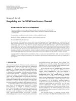
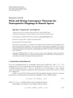
Figure 1: Keystoning removes range walk (top: before Keystoning; bottom: after Keystoning).
motion relative to the platform, whether of the ground itself
or from moving targets embedded within the scene.
Figure 1 shows the effect of Keystoning on the range walk
in a real SAR data collection. The left insets show the range-
time-intensity (RTI) plots while the right insets show the mi-
gration of the peaks in the RTIs over 2 seconds (4000 pulses
at a pulse repetition frequency of 2000 Hz).
If only Keystone formatting was applied, the SAR image
would only be partially focused due to the remaining uncom-
pensated quadratic and the higher-order terms in the target
range. Therefore, after the range walk correction, the SAR
data also has to be compensated for at least the acceleration

to produce reasonably well-focused images.
Even when the radar platform is moving at a constant ve-
locity (in a straight line and at a fixed speed), a point on the
ground experiences a significant pseudo-acceleration with
respect to the phase center of the radar.
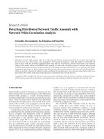
For a simplified first-order analysis, consider the two-
dimensional airborne radar and the ground target geometry
(i.e., the x-y plane contains the line of sight, LOS, and the ve-
locity vector) shown in Figure 2. The platform-centered co-
ordinate system has the x-axis along the longitudinal axis of
the aircraft and y-axis is out the wing. The aircraft is moving
at a velocity v which is along the x-axis.
−10 −50 5 10
x
−v
v
α
R
−5
−4
−3
−2
−1
0
1
2
3
4
5
y

Figure 2: A typical radar-target geometry in SAR.
The range, R, of a point on the ground located at (x,y
axes) is
R
=

x
2
+ y
2

1/2
. (1)
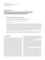
P. K. Sanyal et al. 3
L
AC
Figure 3: The 8-Channel X-band LiMIT system, mounted on a
Boeing 707. L
AC
≈ 18

(source: Lincoln Laboratory briefing, De-
cember 2004).
The radial velocity of the target is then
˙
R
=
x
˙
x + y

˙
y


x
2
+ y
2

=
x
˙
x + y
˙
y
R
,(2)
for the ground-fixed points,
˙
y
= 0, and
˙
x =−v. The range
rate is then
˙
R
=−v
x
R
=−vcos(α), (3)

where α is the angle between the velocity vector and the LOS.
The radial acceleration is then
¨
R
=−v
⎡
⎢
⎣
˙
x


x
2
+ y
2

−
x
x
˙
x



x
2
+ y
2



3
⎤
⎥
⎦
=
−
v
2
R
+
v
2
x
2
R
3
=
v
2
R

cos
2
(α) − 1

.
(4)
For the Lincoln Multimission ISR Testbed (LiMIT, 8
separate subapertures with receivers, operating frequency

9.2GHz, bandwidth 180-MHz, see Figure 3) data discussed
here, R
= ∼22 km, V = ∼208 m/s, and the ground accelera-
tion approaches 2 m/s
2
at α = 90
◦
, that is, at broadside. This
acceleration has considerable effect on the focusing of the
SARimageascanbeseeninFigure 4 .
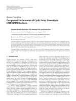
Figure 4 shows a single-channel SAR image resulting
from the RTI shown in Figure 1. (LiMIT SAR data from Fort
Huachuca, Ariz has data from eight subapertures or chan-
nels recorded separately; except for the spatial separations,
all channels are nominally identical.) In this image, only the
Keystone formatting has been applied but no acceleration
correction has been performed yet.
Figure 5 shows the variation of the maximum of SAR im-
age as a function of the acceleration correction applied. It is
seen that for this image the image maximum increases by al-
most 16 dB from zero correction to the optimum accelera-
tion correction of
−2.225 m/s
2
.
−1000 −500 0 500 1000
Cross range (m)
2500
2000
1500

1000
500
Range (m)
20
22
24
26
28
30
32
34
36
38
40
Channel 2; acceleration
= 0m/s
2
;
maximum intensity
= 44.7(dB)
Figure 4: A LiMIT image with Keystoning but without any accel-
eration correction.
00.511.522.533.5
Acceleration (m/s
2
)
80
82
84
86

88
90
92
94
96
98
RDI maximun (dB)
RDI maximun versus acceleration
Figure 5: SAR maximum versus acceleration correction applied to
an image.
Figure 6 shows the image with the optimum acceleration
correction, along with the optical image for the correspond-
ing area as available from Google. Note that the two axes of
the image are shown as “range” and the “cross-range,” with
both units in meters. The cross-range values are obtained
by properly scaling the computed Doppler values. In sub-
sequent images, we have shown the cross-range dimension
as Doppler, which retains the same essential information but
without scaling to meters.
The degree of correspondence between the QuickSAR
image and the optical image is excellent and the major fea-
tures of the QuickSAR image are readily matched to those in
the optical image.
Since each moving target in the scene may have a different
acceleration, the moving targets can be individually further
focused, which would improve their detectability. However,
we have found that adequate detection is possible without the
fine focusing of each target separately. We have used postde-
tection focusing of a target for identification purposes.
4 EURASIP Journal on Advances in Signal Processing

−2000 −1500 −1000 −500 0 500 1000
Cross range (m)
0.5
0
−0.5
−1
−1.5
Range (Km)
RDI; acceleration = 2.225 m/s
2
; [min, max] =−31.8, 98.2(dB)
(a)
(b)
Figure 6: The Acceleration-corrected QuickSAR and the satellite optical image (source: Google).
Boat
(blurred
and offset)
Wake
Figure 7: Boat-off-the-wake (source: www.sandia.gov).
3. MOVING TARGET DETECTION WITH
PHASE INTERFEROMETRY IN QUICKSAR
The process described above produces fairly well-focused
SAR images. Now, given a focused SAR image, how does one
know if any of the detectable objects in the SAR are moving
objects? This can be done via “phase interferometry.”
The target motion causes the moving targets to appear at
locations different from their true instantaneous locations on
the ground in the SAR image. This is due to the coupling of
the cross-range position to the target radial velocity and the
fact that the moving target and the ground under it have dif-

ferent radial velocities relative to the platform. The result is
the well-known “train-off-the-track” where the moving train
appears to be hovering off the image of the track, or the
“boat-off-the-wake” phenomenon (see Figure 7) where the
moving boat is clearly off the tip of the boat wake, where it
really belongs.
3.1. Shift in cross-range due to Doppler processing
How far off is the moving object from its actual location in
a SAR? In the simplified 2D geometry considered above, the
Doppler, f
D
, of a ground point at a small angle θ radians from
the normal to the radar velocity vector is given by
f
D
=
2Vθ
λ
. (5)
If a moving target has the Doppler f
targ
, then it will ap-
pear shifted in cross-range by an angle θ such that
f
targ
=
2Vθ
λ
,
2v

targ
λ
=
2Vθ
λ
,orθ
=
v
targ
V
. (6)
At a range R, this amounts to a linear shift in cross-range,
CrossRangeShift
= Rθ =
Rv
targ
V
. (7)
For the SAR image in Figure 6,wehaveR
≈ 22 km, plat-
form V
≈ 208 m/s. If the target radial velocity v
targ
= 30 m/s
(
≈67.5 mph),
CrossRangeShift
≈
22∗10
3

∗30
208
= 3.173 km. (8)
The upper inset of Figure 8 shows a portion of the SAR
image of the urban area of Fort Huachuca, Ariz. In this
QuickSAR image (2-second integration), one can easily dis-
cern the roads, buildings, and other features of reasonably
large size. There are also other easily detectible, bright ob-
jects. Is there a way to know if any of these other objects are
moving?
3.2. Phase image
To make use of the above-mentioned cross-range displace-
ment phenomenon to detect moving targets in SAR images,
we form a phase-interferometry image as shown in the lower
inset of Figure 8. It is the color-coded plot of the pixel-to-
pixel phase difference between channels one and eight. (The
two end channels of the 8-channel LiMIT system are chosen
P. K. Sanyal et al. 5
(a) SAR image from channel 1
(b) Phase-difference image using channels1and 8
Figure 8: SAR and phase-difference images of Fort Huachuca.
to enhance the phase difference.) The phase difference values
vary between –π and +π,withredfor+π, gradually changing
to blue for –π.
In such an interferometric phase image, all points on the
ground should nominally appear as a continuum of phase
differences from left to right along the cross-range axis. In
Figure 8, we see the fringes parallel to the range direction
gradually changing in color along the cross-range direction.
Pixels of low intensity usually consist of system noise

rather than ground-returns, and hence the channel-to-
channel phase difference becomes unrelated to the indicated
location on the ground and can randomly vary between –π
and +π and the phase-difference image becomes filled with
speckles.
We have arbitrarily set the phase difference values for pix-
els in the SAR which are below a selected dB value (here, it is
10 dB) to –π with the purpose of reducing speckles. Setting
the above LiMIT reduces the speckles. It also helps to delin-
eate areas of low reflectivity, and hence the same features we
see in the SAR (see Figure 8(a)), are also visible in the phase-
difference image (see Figure 8(b)).
Now, while all the points on the ground appear as a
continuum of phase differences along the cross-range axis,
the moving targets appear as discontinuities because a pixel
that represents a moving object appears displaced from the
ground point on which it is instantly situated. This causes a
phase discontinuity. In the color-coded phase difference im-
age, the phase discontinuity shows up as a color anomaly.
By searching for color discontinuities, one can easily iden-
tify several moving targets in the interferometric image. One
such target is circled in red. Thus, the phase-interferometry
image helps to indicate which detected objects in the SAR are
moving objects [5–7]. The color anomaly may not be obvi-
ous in this highly shrunk image but is quite clear in an ex-
ploded version of the image.
3.3. Automated phase discontinuity detection
A trained operator would be able to detect moving targets in
a color-coded phase difference image as described above. For
Figure 9: The General Dynamics Convair 580 belly-mounted

X-band DCS system with one transmit antenna and eight receive
horns.
automated moving target detection, we execute the following
steps:
(a) apply an appropriate acceleration correction to focus
the ground plane;
(b) fit a reference plane, in a least-square error sense, to
the phase difference image;
(c) look for pixels whose phase differences deviation from
the reference plane exceeds a given threshold;
(d) from the above, select those that also exceed an ampli-
tude threshold.
This technique is illustrated with results from another
dataset. This is the General Dynamics DCS 8-Channel, 160-
MHz-bandwidth X-band data from Eglin, Fla (see Figure 9).
In this scenario, there were seven targets moving in circles on
the runway, and the GPS data from the vehicles as well as the
motion data from the radar platform are available.
The top inset in Figure 10 shows a QuickSAR (coherent
processing interval (CPI)
= 0.83 second) of the portion of the
runway where the targets were presented.
6 EURASIP Journal on Advances in Signal Processing
−200 0 200
Doppler (Hz)
150
100
50
0
−50

−100
−150
Range (m)
10
12
14
16
18
20
22
24
26
28
30
SNR (dB)
Clock = 69.41 (s); channel 2; integ. = 0.83 (s);
maximum
= 42.5(dB)
(a)
−200 0 200
Cross range (Doppler, Hz)
150
100
50
0
−50
−100
−150
Range (m)
−3

−2
−1
0
1
2
3
Pre-cancellation phase difference
Clock
= 69.41 (s); shifted = 2.4(rad);
phase difference; channels 2–8; integ.
= 0.83 (s)
(b)
Figure 10: QuickSAR and Phase-difference images of the Eglin Runway.
This QuickSAR is generated from the channel 2 data of
the 8-channel dataset. (Note that the cross-range axis is la-
beled as Doppler in Hz; we did not scale it to meters or az-
imuth angle, but the same information is retained.)
The bottom inset in Figure 10 is the phase-difference im-
age using channels 2 and 5. Note that the runway is still
clearly discernable. The numbers in green indicate the actual
positions of the moving targets at the time the data was col-
lected, while the displaced red numbers indicate where they
should appear in the range-Doppler SAR image. It is inter-
esting to note that target number 5, which is a large target,
shows up more prominently in the phase-difference image
(red circle) than in the QuickSAR image (the color anomaly
is much clearer in a larger display of the image). This vi-
sual observability is very useful to a human operator because
he/she can easily place the detections in the “context” of the
background terrain, that is, whether it is near a building, on a

road, and so forth. Below, we describe how a machine detects
the moving targets.
The blue dots in the upper left inset in Figure 11 are
the row-by-row plots of the phase differences shown in
Figure 10. The red dots (which appear as a line because of
the compactness) are the phases from the plane fitted to the
actual phase differences.
Ideally, all points on the ground would have phase differ-
ences that lie on a plane and only moving targets will have
phase differences that deviate from the plane. But in reality,
because of the system noise, variations in terrain elevation,
and so forth; the actual phase differences, of course, do not
all lie on the plane.
The smaller the clutter power is in a pixel without a target
in it, the more likely it is to be affected by the system noise
and thus more likely to deviate from the plane. The upper
right inset of Figure 11 shows that a very large number of
pixels exceed the selected 1-radian phase deviation threshold
but a significant number of them are below 15 dB. On the
other hand, the pixels corresponding to the moving targets,
we expect to detect, should be of sufficient strength as well as
deviate significantly from the phase plane. Thus, the moving
targets have to meet the dual thresholds: one in power and
the other in phase deviation [8]. If the power threshold is set
at 15 dB in this case, the number of pixels that deviate from
the plane by more than the 1-radian phase deviation thresh-
old drops to 85, as shown in the lower left inset of Figure 11.
The lower right inset in Figure 11 shows these pixels as
the detected targets. These are indicated with red x’s. In this
particular image, there were as many as 85 detections. While

some of these detections are likely to be false alarms, most of
them are possibly multiple detections from “extended,” that
is, large targets.
3.4. Clustering of the detections
An observer can readily group many of these detections into
possible clusters that belong to the same targets. We have
used an automatic clustering algorithm from Matlab, which
results in eight clusters in this image. These clusters are de-
picted with red circles. Note that the circles only indicate the
center of the clustered detections; they do not indicate which
detections belong to the cluster or how many detections were
included in the cluster.
Notice that one cluster coincides with the expected loca-
tion of target number 2, two clusters appear to coincide with
target number 1, four clusters appear to coincide with tar-
get number 5 (which is known to be a large target), and the
eighth cluster appears to comprise one or more false alarms.
A human observer examining the four clusters near target
number 5 or the two near target number 1 would have readily
combined them into single clusters each. The Matlab fuzzy-
logic clustering algorithm used could also possibly have been
tweaked to yield similar results but we did not attempt to do
so at this time.
Zhang et al. also use a dual threshold technique [9]for
detecting slow moving targets in along-track interferometric
P. K. Sanyal et al. 7
−400 −200 0 200 400
Cross range (Doppler, Hz)
−4
−2

0
2
4
Computed phase and
bounded phase difference
dB bounds = (10, 30) dB; ph bounds = (−3.1, 3.1) rad;
regression coefficients
=−2.48555593, 0.00756052, 0.00005026
Slopes not held fixed
(a)
10 15 20 25 30
dB of pixels
−4
−3
−2
−1
0
1
2
3
4
Phase deviation
Pixels over ph threshold = 1rad
Detections
= 40984
(b)
−400 −200 0 200 400
Cross range (Doppler, Hz)
0
0.5

1
1.5
2
2.5
3
3.5
Phase deviations
Pixels over ph threshold = 1rad
and over dB threshold
= 15 dB
Detections
= 85
(c)
−300 −200 −100 0 100 200 300
Cross range (Doppler, Hz)
150
100
50
0
−50
−100
−150
Range (m)
85 dets; 8 clusters; ph threshold = 1(rad);
dB threshold
= 15 (dB); clock = 69.41 (s);
channel 2; integ. = 0.83 (s);
maximum
= 42.5(dB)
(d)

Figure 11: Machine detection of moving targets in a real QuickSAR.
SAR (ATI-SAR). They present results using L-band data from
Jet Propulsion Laboratory (JPL) AirSAR data and show the
successful detection of the breaking waves in the Monterey
Bay area of California. A major difference between the two
methods is that while they talk about a “phase calibration”
which may be affected by the aircraft crab angle, we per-
form a least-square error estimation of the “phase-difference
plane” and do not worry about the minute aircraft motions.
Further, the interferometric technique described here
leads to the direct channel-to-channel clutter cancellation
technique for detecting weaker moving targets.
4. GEOREGISTRATION OF DETECTED MOVING
TARGETS IN QUICKSAR
The “apparent” locations of the moving targets detected in
the SAR image are not their actual locations on the ground.
In fact, recall that the detection of the moving targets in the
SAR image depends on the fact that they are displaced in
cross-range from their actual locations. Therefore, after de-
tection, they need to be “georegistered,” that is, they need to
be placed correctly at their actual locations within the SAR
image. In many applications, a target that is properly georeg-
istered within the SAR has much more intuitive positional
information than the position derived from the range and
angle and converted to latitude/longitude.
Fortunately, the georegistration is almost a byproduct of
the detection process. The top inset in Figure 12 shows the
phase difference of the detected pixels (blue dots) and the
plane fitted to the phase differences of all the ground points
(representedbyreddots,whichhavemergedtoappearasa

line).
Since the moving targets are also on the ground (the
given assumption), the actual locations of the detected pixels
8 EURASIP Journal on Advances in Signal Processing
−400 −200 0 200 400
Cross range (Doppler, Hz)
−3
−2
−1
0
1
2
3
Computed phase plane and
detected phase difference
Pixels over ph threshold = 1rad
and over dB threshold
= 15 dB
Detections
= 85
X
(a)
−300 −200 −100 0 100 200 300
Cross range (Doppler, Hz)
150
100
50
0
−50
−100

−150
Range (m)
Geo-registered; weighted cluster average; ph threshold = 1(rad);
dB threshold
= 15 (dB); clock = 69.41 (s); channel 2;
integ.
= 0.83 (s); maximum = 42.5(dB)
(b)
Figure 12: Geo-registration of moving targets in a real QuickSAR.
are found by displacing them in cross-range until they lie on
the red line, as indicated in the bottom inset of Figure 12.
This displacement may be done on a detection-by-
detection basis or a cluster basis. In a detection-by-detection-
basis georegistration, each detection is moved independently.
As may be obvious, because of the various amounts of noise
in the individual pixels, the pixels that appear to be in a
cluster before georegistration can become scattered after the
above-described displacement.
4.1. Cluster move
Since a clustering has already been performed, it is easy to
move all the detections in a cluster together to appear as the
same cluster after the georegistration. For this, one computes
the average phase difference for the cluster and uses this value
to relocate the whole cluster on the red line.
A slight twist on the above technique is to find a weighted
average of the phase difference using the pixel power to
weight the phase difference values. This plausibly reduces the
effect of low-power pixels which are likely to be noisier.
The right inset in Figure 12 shows the geolocated detec-
tions using the weighted average method. It is seen that the

majority of the detections are now appearing on the runway
where they actually belong.
4.2. Weighted cluster move
Here, we have shown only one image 0.83-second frame of
the dataset from this SAR data collection scenario which lasts
for about 200 seconds. We have applied this technique to the
250 or so frames from this dataset and have obtained consis-
tent detection and georegistration results.
5. DIRECT CHANNEL-TO-CHANNEL CLUTTER
CANCELLATION (DC4) FOR MOVING TARGET
DETECTION
The phase-interferometry technique described above works
well when the target return is strong and well above noise
and ground clutter. In the above examples, we were able to
see the target in the SAR with the naked eye and then used
the phase interferometry to determine if they were moving.
If the moving target return is not significantly stronger
than the ground clutter in that pixel, it will not be noticed
in the phase difference image either because the phase differ-
ence will not be as strongly influenced by the target return.
Clearly, cancelling the clutter will enhance the moving target
detection.
In an ideal case, that is, channels are perfectly balanced,
there is no system noise, there are no moving targets, there
is no internal clutter motion, and so forth, the SAR images
from any two channels only differ in phase that varies linearly
with cross-range or equivalently with Doppler. This phase
difference can be found by simply differencing the two com-
plex images. If all the phase difference values were plotted
against the Doppler, one would see a straight line. And if one

of the images is appropriately weighted by this phase differ-
ence matrix and subtracted from the other, it should result in
a null image, that is, an infinite (in dB) clutter cancellation.
Moving targets, if present, will suffer a cancellation loss but
will not be cancelled completely. The moving target return,
though partly diminished, will be detected with ease.
In a real case, there are system and other sources of noise.
And the lower the clutter return is in a pixel, the more dom-
inated it is by the noise. The upper left inset in Figure 11 is a
plot of the real phase differences (lower insert in Figure 10)
against the Doppler.
The actual distribution of the phase values is not shown
in this plot but a linear trend is clearly visible and in the
absence of any noise (from system or due to internal clut-
ter motion), all phase differences would have collapsed on a
straight line like the red line shown. Indeed, the red line is
the plot of the phases from a plane fitted to the phase values
in Figure 10.
This plane is derived as follows. Consider the phase dif-
ference image as an mxn matrix of phase difference numbers,
P. K. Sanyal et al. 9
−300 −200 −100 0 100 200 300
Cross range (Doppler, Hz)
150
100
50
0
−50
−100
−150

Range (m)
10
12
14
16
18
20
22
24
26
28
30
SNR (dB)
Clock = 69.84 (s); clutter-cancelled image, channel 2;
integ.
= 0.83 (s); maximum = 24.7(dB);
cancellation
= 47.8(dB)
Figure 13: Clutter-cancelled SAR image.
where m is the number of range cells and n is the number of
Doppler cells, that is,
Δϕ(i, j),
range cell i
= 1, , m,
Doppler cell j
= 1, , n.
(9)
We fit a plane to this observed surface:
Δϕ(i, j)
= c

0
+ c
Doppler
j + c
range
i + noise, (10)
where the c’s are the regression coefficients. The phase-
difference plane is primarily sloped in the Doppler dimen-
sion and, therefore, c
Doppler
will have a significant value, but
we also allow the plane to be sloped in the range dimension
and hence the coefficient c
range
.
Having computed the regression coefficients estimates,
we compute the “least-square-fitted” phase difference Δ

φ.In
Figure 11, the red line is the edge view of this fitted plane.
Let the complex images formed at the two channels,
numbered 1 and 8, be designated I
1
and I
8
, respectively. Ide-
ally, (i.e., in the absence of system noise and moving targets)
the images I
1
and I

8
are simply phase-shifted versions of each
other and given the phase shifts, one image can be used to
cancel another. If we now subtract the image from channel 8
weighted by this smoothed phase from the channel 1 image,
we get the clutter-cancelled image
I
1/8
= I
1
− I
8
exp

jΔ

φ

. (11)
Any channel may be cancelled by another channel using
the above method. Figure 13 shows some results of enhanc-
ing moving target return by channel-to-channel cancellation
of the ground clutter and in a channel number 2 image using
the channel number 5 image. (The precancellation channel 2
image, not shown here, appears almost identical to channel
1 precancellation image in the top inset in Figure 10.) Com-
30 40 50 60 70
Pre-cancellation maximum (dB)
20
30

40
50
60
70
80
Cancellation index (dB)
Cancellation index for strongest pixel in each frame
Figure 14: Measured QuickSAR clutter cancellation achieved with
the General Dynamics data.
paring this image with the top inset in Figure 10,itappears
that, as far as the naked eye can tell, almost all of the ground
clutter has been cancelled.
The GD dataset mentioned above contains over 200 sec-
onds of a SAR data run. At about 0.83 seconds of integration
time per QuickSAR, we generated about 250 frames. Each
image was cropped to retain only the area of interest. The
cropped image is 383 range cells
× 661 Doppler cells, thus
containing over a quarter million pixels of various strengths.
It is most likely that each pixel undergoes a different degree
of cancellation and it is worth looking at all pixels to gain
a more thorough picture of the cancellation achieved. How-
ever, for a quick analysis, we only looked at the strongest pixel
from each frame.
We first found the strongest pixel prior to cancellation.
After cancellation, we determine the strength of the same
pixel (not necessarily the strongest in the postcancellation
image) and compute the cancellation. Figure 14 plots the
cancellation ratio that was obtained with this real data (the
red circles are the cancellation values when channel number

2 is cancelled with channel number 5, and the blue dots are
the values when channel number 5 is cancelled with channel
number 8).
Based on only the strongest pixel from each frame, the
average cancellation over the 250 frames is about 37 dB. As a
reference, it is noted that Muehe and Labitt [10]mentiona
clutter-to-noise improvement factor (CIF) of 46 dB with the
MARS radar developed by Lincoln Lab specifically for DPCA
experiments.
We have not done a one-on-one comparison of this clut-
ter cancellation technique with the widely used space time
adaptive processing (STAP) technique [11, 12]forground
clutter cancellation yet. However, it may be noted that with
STAP, one is often concerned about the non-Gaussianity
and nonhomogeneity of the ground clutter. With the direct
channel-to-channel clutter cancellation technique, those is-
sues should not be of concern because each pixel from one
channel is used to cancel the corresponding pixel from the
10 EURASIP Journal on Advances in Signal Processing
other channel and, therefore, how the clutter strength varies
from pixel to pixel is not a major concern.
6. CONCLUSION
In this paper, we have described an interferometric scheme
for detecting and georegistering surface moving targets in
multichannel SAR. The interferometric scheme described
here is able to detect moving targets well within the ground
clutter.
Since the detections take place within a SAR image, and
further, they are properly georegistered, this has the addi-
tional benefits of “contextual” detection, i.e., the detections

are already “in context.” In other words, one can see if they
are on roads, runways, near buildings, and so forth.
We have also described a novel channel-to-channel clut-
ter cancellation technique that enhances the detectability of
moving targets. It has not been exhaustively compared with
the STAP technique but we note that it appears to suffer
less from the non-Gaussian or nonhomogeneous character
of ground clutter in many areas of interest, that is, urban ar-
eas, littoral regions, near forest lines, and so forth.
All the results included here are from real multichannel
radar data that add to the credibility of the techniques.
APPENDIX
KEYSTONE FORMATTING
Keystone formatting can be derived by noting that the spec-
trum of a single-received pulse is given by
S
r
( f ) = P( f )exp

−
i
4π
c

f + f
0

R(t)

,(A.1)

where P( f )
= spectrum of transmitted pulse, f = baseband
frequency (
−B/2 ≤ f<B/2), f
0
= carrier frequency, R(t) =
range to target at time t.
Expanding R(t)inaTaylorseries,weget:
R(t)
= R

t
0

+
˙
R

t
0

t +
1
2
¨
R

t
0


t
2
+ ···.(A.2)
Substituting (A.2) into (A.1) and dropping cubic and
higher-order terms,
S
r
( f )
=P( f )exp

−
i
4π
c

f + f
0

R−i
4π
c

f + f
0

˙
Rt
−i
2π
c


f+ f
0

¨
Rt
2

.
(A.3)
The second term in the brackets containing the product
f
˙
Rt gives rise to range walk. This term becomes zero when
we use the temporal transformation t
= ( f
0
/( f + f
0
))t

.
With the above substitution, (A.3)canbewrittenas
S
r
( f )
=P( f )exp

−
i

4π
c

f+f
0

R−i
4π
c
f
0
˙
Rt

−i
2π
c

f+f
0

¨
R

f
0
t

f+f
0


2

.
(A.4)
Two ta rg e ts
moving
differently
Keystone compensation
Target 1
Target 2
Range cell
Pulse (slow time) no.
Range cell
Target 2
Target 1
Pulse (slow time) no.
Uncompensated
Figure 15: Keystone formatting performs range-walk correction for
all targets moving at different velocities.
Since Keystone formatting does not solve the quadratic
(or higher-order) motion problem, let us also drop the
quadratic term in (A.4) and simplify it to
S
r
( f ) = P( f )
∗
exp

−

i
4π
c

f + f
0

R − i
4π
c
f
0
˙
Rt


.
(A.5)
The Keystone process compensates for the different ra-
dial velocities of all moving targets simultaneously. Figure 15
shows the result of a first-order simulation to illustrate how
targets moving at two different velocities are simultaneously
corrected for range-walk.
ACKNOWLEDGMENTS
The authors would like to thank AFRL Rome Research Site
in Rome, NY for providing them with the various real radar
data sets used in their work. They would also like to thank
the anonymous reviewers for their detailed critiques which
helped to greatly improve this paper.
REFERENCES

[1] I.G.CummingandF.H.Wong,Digital Processing of Synthetic
Aperture Radar Data, Artech House, Boston, Mass, USA, 2005.
[2]R.P.Perry,R.C.DiPietro,andR.L.Fante,“SARimagingof
moving targets,” IEEE Transactions on Aerospace and Electronic
Systems, vol. 35, no. 1, pp. 188–199, 1999.
[3] R. P. Perry, R. C. DiPietro, and R. L. Fante, “Coherent integra-
tion with range migration using keystone formatting,” in Pro-
ceedings of IEEE Conference on Radar (RADAR ’07), pp. 863–
868, Waltham, Mass, USA, April 2007.
[4] E.F.StockburgerandD.N.Held,“Interferometricmovingtar-
get imaging,” in Proceedings of the IEEE International Radar
Conference, pp. 438–443, Arlington, Va, USA, May 1995.
[5] P. K. Sanyal, R. P. Perry, and D. M. Zasada, “Detecting mov-
ing targets in SAR via keystoning and phase interferome-
try,” in Proceedings of the 5th International Radar Symposium
(IRSI ’05), Bangalore, India, December 2005.
[6] P. K. Sanyal, D. M. Zasada, and R. P. Perry, “Detecting mov-
ing targets in SAR via keystoning and multiple phase center
interferometry,” in Proceedings of IEEE Conference on Radar
(RADAR ’06), pp. 498–503, Verona, NY, USA, April 2006.
P. K. Sanyal et al. 11
[7] D. M. Zasada, P. K. Sanyal, and R. P. Perry, “Detecting moving
targets in clutter in airborne SAR via keystoning and multiple
phase center interferometry,” in Algorithms for Synthetic Aper-
ture Radar Imagery XIII, vol. 6237 of Proceedings of SPIE,pp.
1–8, Orlando, Fla, USA, April 2006.
[8] D. M. Zasada, P. K. Sanyal, and R. P. Perry, “Detecting moving
targets in multiple-channel SAR via double thresholding,” in
Proceedings of the IET International Conference on Radar Sys-
tems, Edinburgh, UK, October 2007.

[9] Y. Zhang, A. Hajjari, K. Kim, and B. Himed, “A dual-threshold
ATI-SAR approach for detecting slow moving targets,” in Pro-
ceedings of IEEE International Radar Conference (RADAR ’05),
pp. 295–299, Washington, DC, USA, May 2005.
[10] C. E. Muehe and M. Labitt, “Displaced-phase-center antenna
technique,” Lincoln Laboratory Journal, vol. 12, no. 2, pp. 281–
296, 2000.
[11] J. Ward, “Space-time adaptive processing for airborne radar,”
Tech. Rep. ESC-TR-94-109, MIT Lincoln Laboratory, Lexing-
ton, Mass, USA, 1994.
[12] P. K. Sanyal, “STAP processing monostatic and bistatic
MCARM data,” Tech. Rep. AFRL-SN-RS-TR-1999-197,
MITRE Corporation, Bedford, Mass, USA, 1999.