Báo cáo hóa học: " Research Article Constructing Battery-Aware Virtual Backbones in Wireless Sensor Networks" docx

Hindawi Publishing Corporation
EURASIP Journal on Wireless Communications and Networking
Volume 2007, Article ID 40154, 15 pages
doi:10.1155/2007/40154
Research Article
Constructing Battery-Aware Virtual Backbones in
Wireless Sensor Networks
Chi Ma,
1
Yuanyuan Yang,
2
and Zhenghao Zhang
3
1
Department of Computer Science, Stony Brook University, Stony Brook, NY 11794, USA
2
Department of Electrical and Computer Engineering, Stony Brook University, Stony Brook, NY 11794, USA
3
Department of Computer Scie nce, Carnegie Mellon University, 5000 Forbes Avenue, Pittsburgh, PA 15213-3891, USA
Received 14 October 2006; Accepted 13 March 2007
Recommended by Lionel M. Ni
A critical issue in battery-powered sensor networks is to construct energy efficient virtual backbones for network routing. Recent
study in battery technology reveals that batteries tend to discharge more power than needed and reimburse the over-discharged
power if they are recovered. In this paper we first provide a mathematical battery model suitable for implementation in sensor
networks. We then introduce the concept of battery-aware connected dominating set (BACDS) and show that in general the
minimum BACDS (MBACDS) can achieve longer lifetime than the previous backbone structures. Then we show that finding a
MBACDS is NP-hard and give a distributed approximation algorithm to construct the BACDS. The resulting BACDS constructed
by our algorithm is at most (8 + Δ)opt size, where Δ is the maximum node degree and opt is the size of an optimal BACDS.
Simulation results show that the BACDS can save a significant amount of energy and achieve up to 30% longer network lifetime
than previous schemes.
Copyright © 2007 Chi Ma et al. This is an open access article distributed under the Creative Commons Attribution License, which

permits unrestricted use, distribution, and reproduction in any medium, provided the original work is properly cited.
1. INTRODUCTION
A sensor network is a distributed wireless network which is
composed of a large number of self-organized unattended
sensor nodes [1–3]. Sensor nodes, which are small in size and
communicate untethered in short distance, consist of sens-
ing, data processing, and communication components with
limited battery supply. Applications of sensor networks range
from outer-space exploration, medical treatment, emergency
response, battlefield monitoring to habitat, and seismic ac-
tivity monitoring. A typical function of sensor networks is
to collect data in a sensing environment. Usually the sensed
data in such an environment is routed to a sink, which is
the central unit of the network [4–6]. Although a sensor net-
work does not have a physical infrastructure, a virtual back-
bone can be formed by constructing a connected dominat ing
set (CDS) [7–9] in the network for efficientpacketrouting,
broadcasting, and data propagating.
In general, a sensor network can be modeled as a graph
G
= (V, E), where V and E are the sets of nodes and edges in
G, respectively. A CDS is a connected subgraph of G where all
nodes in G are at most one hop away from some node in the
subgraph. Figure 1 shows a C DS for a given sensor network.
In this example, packets can be routed from the source (node
I) to a neighbor in the CDS (node G), along the CDS back-
bone to a dominating set member (node D), which is closest
to the destination (node B), and then finally to the destina-
tion. A node in the CDS is referred to as a dominator,and
a node not in the CDS is referred to as a dominatee.There

has been a lot of work that dedicates to construct a mini-
mum connected dominating set (MCDS) which is a CDS with
a minimum number of dominators. Unfortunately, finding
such an MCDS in a general graph was proven to be NP-hard
[10, 11]. So was in a unit disk graph (UDG) [12], where nodes
have connections only within unit distance. Approximation
algorithms were proposed to construct CDS, see, for exam-
ple, [13–15]. The CDS computed by these algorithms has at
most 8 opt
MCDS
size, where opt
MCDS
is the size of the MCDS.
Although previous CDS construction algorithms achieve
good results in terms of the size of the CDS, a minimum size
CDS does not necessarily guarantee the optimal network per-
formance from an energy efficient point of view. The MCDS
model assumes that the battery discharging of a sensor node
is linear, in other words, the energy consumed from a battery
is equivalent to the energy dissipated in the device. However,
research has found that this is a rather rough assumption on
2 EURASIP Journal on Wireless Communications and Networking
A
B
C
D
E
F
G
H

I
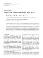
Figure 1: The minimum connected dominating set (MCDS)
{C, D, F, G} forms a backbone for the sensor network. A packet is
forwarded from node I to node B by the backbone.
the real sensor batteries [16–19]. Recent study on battery be-
havior reveals that, unlike what we used to believe, batteries
tend to discharge more power than needed, and reimburse
the over-discharged power later if they have appropriate rests
[16–18]. The process of this reimbursement is referred to as
battery recovery. In this paper, we will present a mathemati-
cal battery discharging model, which is independent of bat-
tery chemistry. This model can accurately model the battery
discharging/recovery behavior with online computable func-
tions for implementing in wireless ad hoc networks. Based on
this model, we will introduce battery-aware connected domi-
nating set (BACDS) and show that the BACDS can achieve
better network p erformance than the MCDS.
The rest of the paper is organized as follows. In Section 2,
we discuss some background and related work to place our
work in context. We study the mathematical battery model
in detail and present a simplified model suitable for sensor
network applications in Section 3. Section 4 first gives the
BACDS model along with its performance comparison with
the MCDS model, then presents a distributed approximation
algorithm to construct the BACDS. We also analyze the per-
formance of the algorithm and give an upper bound on the
size of the BACDS obtained in this section. Finally, we give
simulation results in Section 5 and concluding remarks in
Section 6.
2. BACKGROUND AND RELATED WORK

Before constructing the battery-aware CDS, in this section,
we provide some background on battery models and existing
CDS construction algorithms.
2.1. Modeling battery discharge behavior
The most commonly used batteries in wireless devices and
sensors are nickel-cadmium and lithium-ion batteries. In
general, a battery consists of cells arranged in series, paral-
lel, or a combination of both. Two electrodes: an anode and
a cathode, separated by an electrolyte, constitute the active
material of each cell. When the cell is connected to a load, a
reduction-oxidation reaction transfers electrons from the an-
ode to the cathode. To illustrate this phenomenon, Figure 2
shows a simplified symmetric electrochemical cell. In a fully
charged cell (Figure 2(a)), the electrode surface contains the
maximum concentration of active species. When the cell is
connected to a load, an electrical current flows through the
external circuit. Active species are consumed at the electrode
surface and replenished by diffusion from the bulk of the
electrolyte. However, this diffusion process cannot keep up
with the consumption, and a concentration gradient builds
up across the electrolyte (Figure 2(b)). A higher load elec-
trical current I results in a higher concentration gradient
and thus a lower concentration of active species at the elec-
trode surface [20]. When this concentration falls below a cer-
tain threshold, the electrochemical reaction can no longer
be sustained at the electrode surface and the charge is un-
available at the electrode surface (Figure 2(e)). However, the
unused charge is not physically “over-consumed,” but sim-
ply unavailable due to the lag between the reaction and the
diffusion rates. If the battery current I is reduced to zero

or a very small value, the concentration gradient flattens
out after a sufficiently long time, reaching equilibrium again
(Figure 2(c)). The concentration of act ive species near the
electrode surface following this recovery period makes un-
used charge available again for extraction (Figure 2(d)). We
refer to the unused charge as discharging loss.Effectively re-
covering the battery can reduce the concentration gradient
and recover discharging loss, hence, prolong the lifetime of
battery (Figure 2(f)). Experiments on nickel-cadmium bat-
tery and lithium-ion battery show that the discharging loss
might take up to 30% of the total battery capacity [19].
Hence, precisely modeling battery behavior is essential for
optimizing system performance in sensor networks.
Researchers have developed high-level mathematical
models that capture the battery behavior and are indepen-
dent of battery chemistry [17–19]. An analytical battery
model was proposed in [19], however, this model requires
long computing time and large precomputed look up ta-
bles. We therefore provided a discrete time battery model in
[17, 18] with online computable functions. This model splits
the time into discrete time slots with a fixed slot length and is
suitable for packetized ad hoc networks. We will discuss this
modelinmoredetailinSection 3.
2.2. Distributed algorithms for MCDS construction
As we discussed in Section 1, CDS is the virtual backbone
of a wireless sensor network. Packets route through CDS to
the sink or to other s ensors. A non-CDS network is a net-
work that does not adopt CDS as backbone, which would re-
duce its overall performance as indicated in previous research
[9, 21]. Algorithms for constructing CDS in wireless sensor

networks have been studied by several researchers [21, 22].
The first algorithm reported in [22] is a greedy heuristic al-
gorithm with bounded performance guarantees. In this algo-
rithm, initially all nodes are colored white. The CDS is grown
from one node outward by coloring black those nodes that
have maximum number of white neighbors. This algorithm
yields a CDS of size at most 2(1 + H(Δ)) opt
MCDS
,whereH is
the harmonic function and Δ is the maximum node degree.
Das, et al. proposed an algorithm based on [22] by selecting a
node with the maximum degree as the root of a spanning tree
T, then repeatedly running the coloring procedure to form
the spanning tree [9]. This algorithm has an approximation
Chi Ma et al. 3
Electrolyte
Electrode
Electroactive species
(a) Fully charged state
Electrolyte
Electrode
Diffusion
Consumption
Electroactive species
(b) In discharging
Electrolyte
Electrode
Diffusion
Electroactive species
(c) In recovery

Electrolyte
Electrode
Electroactive species
(d) After recovery
Electrolyte
Electrode
Electroactive species
Discharging loss
Battery di es as no species
reaches the electrolyte
(e) Battery dies with discharging loss
Electrolyte
Electrode
Energy fully consumed
(f) Battery dies without discharging loss
Figure 2: Batter y operation at different states.
ratio of O(log Δ) for a general graph. However, these algo-
rithms are centralized algorithms, which makes their appli-
cations quite limited.
Distributed algorithms for CDS constructions have been
proposed in recently years. They can be categorized as
WCDS-based, Pruning-based and MIS-based, approaches. In
these distributed algorithms, each node in the network is
assigned a unique ID. The weakly connected dominating set
(WCDS) is a dominating set of graph G such that WCDS and
its neighbors induce a connected subgraph of G. In a WCDS,
the nodes are partitioned into a set of cluster heads and clus-
ter members, such that each cluster member is within the ra-
dio range of at least one cluster head. In the algorithm pro-
posed in [23], nodes elect their neighbor with the lowest ID

as their cluster head. Whenever a node with a lower ID moves
into the range of a cluster head, it becomes the new cluster
head. A problem of this algorithm is that the cluster structure
is very unstable: when a lower ID node moves in, a cluster
may break into many subclusters. Apparently, this reorgani-
zation is unnecessary in many situations.
Pruning-based approaches construct a CDS first and
then prune the redundant nodes from this CDS [9]. In a
pruning-based algorithm, any node having two disconnected
neighbors is marked as a dominator. The redundant domi-
nator set is post-processed by pruning nodes out of the CDS.
The closed neighbor set of node u is defined as the set of u’s
neighbors plus u itself. A node u is pruned out if there exists
anodev with higher ID such that the closed neighbor set of
u is a subset of the closed neighbor set of v. Unfortunately,
the theoretical bound on the resulting CDS obtained by this
algorithm remains unspecified.
Minimum independent set (MIS) is an independent set
such that adding any new node to the set breaks the inde-
pendence property of the set. Thus, every node in the graph
is adjacent to some node in the MIS. MIS-based algorithms
construct a CDS by finding an MIS and then connect it.
4 EURASIP Journal on Wireless Communications and Networking
References [13, 15] gave an algorithm for unit disk graphs
with performance bounds. It first constructs a rooted span-
ning tree in G, then a labeling process begins from the root
to the leaves by broadcasting “Dominator/Dominatee” mes-
sages to form the MIS. The final phase connects the nodes in
the MIS to form a CDS. The algorithm has time and mes-
sage complexities of O(n)andO(n logn), respectively, for

an n-node graph. The resulting CDS has a size of at most
8opt
MCDS
. Reference [14] presented a multileader MIS-based
algorithm by rooting the CDS in multiple sources. Its perfor-
mance ratio is 192
|opt
MCDS
| +8.
All the existing MCDS algorithms assume that the bat-
tery discharging of a sensor node is linear. This is a rough
assumption as shown in Section 2.1, and it does not necessar-
ily guarantee the optimal network performance from an en-
ergy efficient point of view. In the following sections we will
introduce an accurate battery model to describe the battery
discharging behavior. Then we will use this battery model to
construct energy efficient virtual backbones in wireless sen-
sor networks.
3. BATTERY DISCHARGING MODELS
The battery discharging model presented in [17, 18]isan
online computable model for general ad hoc wireless net-
works. In this section, we further reduce the computational
complexity to make it implementable in sensor networks.
We assume that a battery is in discharging during time
[t
begin
, t
end
] with current I. The consumed power α is calcu-
lated in [17, 18]as

α
= I ×

t
end
− t
begin

+ I ×
π
2
3β
2
×

e
−β
2
(t−t
end
)
− e
−β
2
(t−t
begin
)

,
(1)

where t is the current time and β is a constant parameter. The
right-hand side of (1) contains two components. The first
term, I
×(t
end
−t
begin
), is simply the energy consumed in de-
vice during [t
begin
, t
end
]. The second term is the discharging
loss in [t
begin
, t
end
] and it decreases as t increases. The con-
stant β (> 0) is an experimental chemical parameter which
may be different from battery to battery. In general, the larger
the β, the faster the battery diffusion rate, hence, the less the
discharging loss.
In ad hoc networks, current I is a continuous variable
for various applications such as operating systems, multi-
media transmission, word processing, and interactive games.
However, in sensor networks, the simple sensing and data
propagating activities of sensor nodes may only require sev-
eral constant currents [24]. We define the constant currents
of dominator nodes and dominatee nodes as I
d

and I
e
,re-
spectively. A dominator needs to keep active and listen to all
channels at all times. Compared with I
d
, the I
e
of a domi-
natee is very low. We divide the sensor lifetime into discrete
time slots with slot length δ. In each time slot, the battery
of a node is either as a dominator (I
= I
d
) or a dominatee
(I
= I
e
). Figure 3(a) shows the discrete time activities on a
0
δ
t
0
Time slot
123456
I
e
I
d
Current (I)

Discharging slot
(a)
t
0
κ
1
= 5
Ignored recovery
slots
Time
slot
ζ
1
(5δ)
ζ
1
(4δ)
ζ
1
(3δ)
ζ
1
(2δ)
ζ
1
(1δ)
Recovery capacity
(mAmin)
ζ
1

(t)
ζ
1
(4δ) is permanently
lost if sensor
dies at t
0
The power to
transmit a packet
c
(b)
(c) Recovery table
m
= 4, i = 2, κ
2
< (m − i)
Entry 2 should be remov ed
Time slot (i)
1
2
3
κ
i
5
1
1
Current (I)
1
0
0

Figure 3: The discharging of a sensor battery. (a) The node is a
dominator in slots 1 and 5 and dominatee in slots 2, 3, 4, and 6. (b)
The capacity ζ
1
(t) is discharged in slot 1 and recovered gradually in
the following slots. ζ
1
(t) after slot 6 is ignored. If this battery dies in
slot 5, ζ
1
(4δ) is permanently lost. (c) The recovery table records the
recovery status κ
i
at m = 4. The 0 and 1 in the current column stand
for I
d
and I
e
,respectively.
sensor node, where ζ
n
(t) is the discharging loss in the nth
time slot [(n
− 1)δ, nδ], n ≥ 1. From (1), we have
ζ
n
(t) = I
n
×
π

2
3β
2

e
−β
2
(t−nδ)
− e
−β
2
(t−(n−1)δ)

,(2)
where I
n
is either I
d
or I
e
,andt is the current time.
We can see that ζ
n
(t) is recovered gradually in the follow-
ing (n+1)th,(n+2)th, slots until t. It should be mentioned
that discharging loss ζ
n
(t) is only a potentially recoverable
energy. In Figure 3, if the battery dies at the 5th slot, the en-
ergy ζ

1
(4δ), , ζ
4
(4δ) do not have a chance to be recovered.
Thus, the battery permanently loses them. At time t, the gross
discharging loss energ y of this battery is
ζ(t)
=
m

i=1
ζ
i
(t), (3)
where m
=t/δ. The lower the ζ(t)is, the better the bat-
tery is recovered. To be aware of the battery recovery status,
ζ(t) needs to be calculated at each slot. However, the com-
putation can be simplified by observing that ζ
i
(t)decreases
exponentially as t increases. Naturally, ζ
i
(t) can be ignored if
ζ
i
(t) is less than a small amount of power c,wherec is the
power to transmit a single packet. We introduce κ
i
such as

Chi Ma et al. 5
Table 1: The maximum size of the recovery table (β = 0.4).
c/I
d
1200 mA 800 mA 400 mA 100 mA
200 mAmin 1234
400 mAmin
2335
600 mAmin
3346
800 mAmin
3456
ζ
i
(κ
i
δ) <c<ζ
i
((κ
i
− 1)δ), that is, after t = κ
i
δ, ζ
i
(t)isig-
nored. We have
κ
i
=


1
β
2
δ
log
π
2

1 − e
−β
2
δ

3β
2
c/I
i

,(4)
where I
i
= I
d
or I
e
. We maintain κ
i
in a recovery table. At the
mth slot, if κ
i

< (m −i), which indicates that ζ
i
(mδ) <c, then
this entry i is removed from the table. An example is given in
Figure 3(c) where the second entr y is about to be removed.
Introducing this recovery table has several advantages
and is also feasible for sensor networks. First, we can reduce
the computational complexity of battery-awareness. Only the
remained entries in the table are used for computing ζ(t).
Now (3)canberewrittenas
ζ(t)
=

j
ζ
j
(t), (5)
where entry j is the entry remained in the recovery table. Sec-
ond, we can reduce the complexity of table maintenance. In
order to check whether an entry needs to be removed, rather
than calculating ζ
i
(t)foreveryi at each time, we only need
to read κ
i
from the table and compare it with m.Becauseκ
i
is computed once, maintaining the recovery table is simple.
Third, the size of the table is feasible for sensor memory. Ac-
cording to (4)and(5), the total entries in the recovery ta-

ble are no more than
(1/β
2
δ)log(π
2
(1 − e
−β
2
δ
)/3β
2
c/I
d
).
For various possible values of I
d
and c of sensors, Table 1
shows the maximum number of entries in a recovery table
(β
= 0.4). Considering that the memory capacity of today’s
sensor node is typically larger than 512 KB [25, 26], it is ac-
ceptable to store and maintain such a recovery table in sensor
memory. Thus, we can reduce the computational complexity
by maintaining a recovery table on a sensor node with a fea-
sible table size.
In summary, in this section we use the battery model to
achieve battery-awareness by capturing its recovery ζ(t). The
lower the ζ(t), the better the sensor node is recovered at time
t. We introduce the recovery table to reduce the computa-
tional complexity. We also show that maintaining such a table

is feasible for today’s sensor nodes. Next we apply this battery
model to construct the BACDS to prolong network lifetime.
4. BATTERY-AWARE CONNECTED DOMINATING SET
In this section, we first introduce the concept of battery-
aware connected dominating set (BACDS), and show that
MCDS algorithm:
Repeat
Every node i with P
residual
(i) ≥ P
threshold
is marked as qualified;
All other nodes are marked as unqualified;
Call MCDS construction algorithm for all qualified nodes;
If successful, use the MCDS constructed as the backbone;
Otherwise report “no backbone can be formed” and exit;
Until Some dominator j has P
residual
( j) <P
threshold
;
BACDS algorithm:
Repeat
Every node i with P
residual
(i) ≥ P
threshold
is marked as qualified;
All other nodes are marked as unqualified;
Call BACDS construction algorithm for all qualified nodes;

If successful, use the BACDS constructed as the backbone;
Otherwise report “no backbone can be formed” and exit;
Until δ time has elapsed or some dominator j has
P
residual
( j) <P
threshold
;
Algorithm 1: Outline of MCDS and BACDS algorithms for form-
ing a virtual backbone.
the BACDS can achieve better network performance. Then
we provide a distributed algorithm to construct BACDS in
sensor networks.
4.1. Battery-aware dominating
Let the sensor network be represented by a graph G
= (V, E)
where
|V|=n. For each pair of nodes u, v ∈ V,(u, v) ∈ E if
and only if nodes u and v can communicate in one hop. The
maximum node degree in G is Δ.Eachnodev is assigned a
unique ID
v
. P
residual
(v)isv’s residual battery power. P
threshold
is the threshold power adopted in CDS construction algo-
rithms. ζ
v
(t) is the discharging loss of v at time t.Forany

subset U
⊆ V,wedefineζ
U
max
= max {ζ
v
(t) | v ∈ U}.
Next we explain how to use the battery model to con-
struct an energy-efficient dominating set in a sensor network.
Intuitively, longer network lifetime can be achieved by always
choosing the “most fully recovered” sensor nodes as domina-
tors. For a graph G
= (V, E)attimet,wedefineaBACDSas
asetS
B
(⊆ V) such that
S
B
is a CDS of G, ζ
S
B
max
= min

ζ
S
max
| S is a CDS of G

.

(6)
An optimal BACDS is a BACDS with a minimum number
of nodes and is denoted as MBACDS. For notational conve-
nience, we let
ζ
BACDS
≡ min

ζ
S
max
| S is a CDS of G

. (7)
BACDS can achieve better performance than MCDS since
it balances the power consumption among sensor nodes.
Algorithm 1 gives the outline of the MCDS and BACDS
6 EURASIP Journal on Wireless Communications and Networking
0 10203040506070
Network lifetime (min)
0
0.1
0.5
1
1.5
2
2.5
3
3.5
4

4.5
5
Residual capacity of sensor battery (mAmin)
Threshold
{C, D, F,G}
{C, D, F,G}
{A, B, E, H}
{A, B, E, H}
BACDS set1
MCDS set1
MCDS set2
BACDS set2
Network lifetime under BACDS and MCDS models
Figure 4: The sensor network in Figure 1 achieves longer lifetime
using the BACDS model than the MCDS model. The results were
simulated with the battery discharging model. In this case, the net-
work lifetime is prolonged by 23.2% in the BACDS model.
A
B
C
D
E
F
G
H
I
{A, B, E, H, I}: ζ
= 0
{C, D, F,G}: ζ
= 2.1 × 10

4
mAmin
Figure 5: The battery-aware connected dominating set (BACDS)
for the network in Figure 1 at t
= 10 minutes. The ζ
i
(t)foreach
node i is listed above.
algorithms for forming a virtual backbone in a sensor net-
work, where node i is qualified to be selected as a dominator
as long as its residual battery power P
residual
(i) is no less than
the threshold power P
threshold
.
We conducted simulations to compare the two algo-
rithms. Figure 4 shows the simulated lifetime under BACDS
and MCDS models for the network in Figure 1. At the
beginning, all nodes are identical with battery capacity C
=
4.5 × 10
4
mAmin and β = 0.4. The discharging currents
are I
d
= 900 mA and I
e
= 10 mA. An MCDS is chosen as
Set

1
={C, D, F,G} (Figure 1 ). Since MCDS does not con-
sider the battery behavior, Set
1
remains as the dominator
until the power of all nodes in Set
1
drops to a threshold
0.1
× 10
4
mAmin. After that, another MCDS is chosen as
Set
2
={A, B, E, H}.AfterSet
2
uses up its power, no node
in the network is qualified as a dominator. The total network
lifetime is 56 min (Figure 4).
On the other hand, in the BACDS model a CDS is formed
by the nodes with minimum ζ(t)s. The network reorganizes
(1) Find a subset SET
+
in G;
(2) Construct a subset COV in SET
+
;
/
∗
COV covers the nodes in V −SET

+
∗
/
(3) Construct a subset CDS
+
in SET
+
;
/
∗
CDS
+
is the CDS of SET
+
∗
/
SET
0
= COV ∪CDS
+
is a BACDS;
Algorithm 2: The outline of the BACDS construction.
the BACDS for every δ time. Suppose at the beginning the
BA CDS is still Set

1
={C, D, F,G}.Afterδ = 10 min, the
power of nodes in Set

1

is reduced to 2.1 × 10
4
mAmin. At
this time, a new BACDS is chosen as Set

2
={A, B, E, H}
(Figure 5). During the next 10 minutes, Set

2
dissipates the
power to 2.1
× 10
4
mAmin while Set
1
recoveries its nodes’
power from 2.1
×10
4
mAmin to 3.35×10
4
mAmin. Then the
BACDS is organized again. As shown in Figure 4, the total
network lifetime in the BACDS model is 69 minutes, which
is 23.2% longer than the MCDS model.
We have seen that BACDS can achieve longer lifetime
than MCDS. Next we wi ll consider the BACDS construction
algorithm.
4.2. Formalization of BACDS construction problem

The BACDS construction problem can be formalized as fol-
lows: given a graph G
= (V, E)andζ
i
(t)foreachnodei in G,
find an MBACDS. For simplicity, we use ζ to denote ζ(t)in
the rest of the paper. First, we have a theorem regarding the
NP-hardness of the problem.
Theorem 1. Finding an MBACDS in G is NP-hard.
Proof. Consider a special case that all nodes in G have the
same ζ values. In this case, finding an MBACDS in G is equiv-
alent to finding an MCDS in G. Since the MCDS problem is
NP-hard, the MBACDS problem is also NP-hard.
Now since the MBACDS construction is NP-hard, we will
construct a BACDS by an approximation algorithm. By def-
inition, the BACDS to be constructed, S
B
, must satisfy the
following two conditions: (i) ζ
S
B
max
= ζ
BACDS
; (ii) S
B
is a CDS
of G. Also, the size of S
B
should be as small as possible.

Our algorithm is designed to find a set to satisfy these
conditions. To satisfy condition (i), the algorithm finds a
subset SET
+
in G, such that for any subset S

(⊆ SET
+
),
ζ
S

max
≤ ζ
BACDS
. We will prove that, as long as a set S

(⊆ SET
+
)
is a CDS of G, we can guar antee that ζ
S

max
= ζ
BACDS
.
To satisfy condition (ii), the algorithm will find two sets:
CDS
+

and COV, both in SET
+
.CDS
+
(⊆ SET
+
)isanMCDS
of SET
+
.COV(⊆ SET
+
)isacoverofV − SET
+
,which
dominates all the nodes in V
− SET
+
. We will prove that
SET
0
= COV ∪ CDS
+
is the BACDS we want. The detailed
algorithm will be presented in Section 4.3 . Algorithm 2 gives
an outline of the BACDS construction algorithm.
Chi Ma et al. 7
We now show that SET
0
= COV ∪ CDS
+

is indeed a
BA CDS.
Theorem 2. SET
0
= COV ∪CDS
+
is a BACDS.
Proof. We first define SET
+
as
SET
+
=

v ∈ V | ζ
v
≤ ζ
BACDS

. (8)
We know that CDS
+
is a CDS of SET
+
and COV dominates
the nodes in V
− SET
+
.ToproveSET
0

= COV ∪ CDS
+
is a
BACDS, we need to show that set SET
0
is a connected domi-
nating set of G,andζ
SET
0
max
is minimized.
First, we show that SET
0
is connected. Because COV ⊆
SET
+
, every node in COV is at most one hop away from
CDS
+
. Also, since CDS
+
is connected, SET
0
= COV ∪CDS
+
is connected.
Second, we prove that SET
0
is a dominating set of G.
Since CDS

+
is a CDS of SET
+
,allnodesinSET
+
are domi-
nated by CDS
+
. Also, since all nodes in V −SET
+
are covered
by COV, SET
0
= COV ∪CDS
+
is a dominating set of G.
Finally, we show that ζ
SET
0
max
is minimized, that is, ζ
SET
0
max
=
ζ
BACDS
.Since SET
0
⊆ SET

+
={v ∈ V | ζ
v
≤ ζ
BACDS
},
we hav e ζ
SET
0
max
≤ ζ
BACDS
.However,SET
0
is also a CDS of G.
Thus, ζ
SET
0
max
≥ ζ
BACDS
. Therefore, ζ
SET
0
max
= ζ
BACDS
,andwehave
proved that SET
0

= COV ∪CDS
+
is a BACDS.
In summary, in this subsection we have shown that we
can construct a BACDS by finding three subsets SET
+
,COV,
and CDS
+
step by step. Then SET
0
= COV ∪ CDS
+
is a
BACDS. Next we will give the algorithms to construct SET
+
,
COV, and CDS
+
.
4.3. A distributed algorithm for BACDS construction
Our algorithm for BACDS construction consists of three pro-
cedures for constructing SET
+
and COV in G. In the algo-
rithm, we use N(v) to denote the set of neighbor nodes of
v. each node is colored in one of the three colors: black,
white, and gray. N
black
(v), N

white
(v), and N
gray
(v) are the sets
of black, white, and gray neighbors of v, respectively. Also we
use sets list
gray
(i) and list(i) to store the neighbor information
for node i.
First we consider the construction of SET
+
.TofindSET
+
,
we do the following: the ζ
i
of each node i in G is collected in
the sink; then the sink calculates ζ
SET
+
max
and broadcasts it in
a beacon; on receiving the beacon, all nodes with ζ
i
≤ ζ
SET
+
max
form set SET
+

.TheprocedureisdescribedinAlgorithm 3.
Initially, all nodes in G are colored gray. Then the algorithm
colors some gray nodes black. In the end, the set of black
nodes is SET
+
.
Note that in SET
+
finding procedure, the sink collects in-
formation from sensors only once, and broadcasts the ζ
SET
+
max
in a single beacon. The overhead of information collecting
and broadcasting is minimum.
Now we consider the construction of COV. This problem
of constructing a minimum size COV can be formulated as
the following given two graphs
G
1
and G
2
.NodesinG
1
and
G
2
are interconnected with edges. A minimum size COV is to
be found in
G

1
such that G
2
⊆ N(G
1
). We show that finding a
(1) All nodes in G are colored gray;
(2) Each gray node i in the network does the following:
(3) begin
(4) Broadcast a packet which includes its ID
i
;
(5) Receive neighbors’ IDs;
(6) Calculate ζ
i
;
(7) Route a packet with (ID
i
,ID
N(i)
, ζ
i
) to the sink;
(8) Listen to the beacon for ζ
SET
+
max
;
(9) if ζ
i

≤ ζ
SET
+
max
then node i is colored black;
(10) end;
(11) The sink does the following:
(12) begin /
∗
Calculate ζ
SET
+
max
∗
/
(13) Collect packets from sensor nodes;
(14) S
0
:={ζ
i
| i = 1, 2, , n};
(15) S
1
:=∅;
(16) repeat
(17) S
2
:={those nodes with the smallest ζ in S
0
};

(18) S
0
:= S
0
− S
2
;
(19) S
1
:= S
1
∪ S
2
;
(20) until S
1
is a CDS or S
0
=∅;
(21) if S
1
is a CDS then
(22) ζ
SET
+
max
:= ζ
S
1
max

;
(23) Broadcast ζ
SET
+
max
in a beacon;
(24) end if ;
(25) else report “no CDS can be found”
(26) end;
SET
+
:={black nodes };
Algorithm 3: SET
+
finding procedure.
minimum size COV is NP-hard even in an UDG graph. If we
can show that this problem is NP-hard in an UDG, it is clear
that this problem is also NP-hard in a general graph. We have
the following theorem regarding its NP-hardness.
Theorem 3. Finding a minimum COV in an UDG is NP-hard.
Proof. To see this, we use the fact that it is NP-hard to find
a minimum dominating set in an UDG. Given any UDG
instance, say,
G, which has vertex set V ={v
1
, v
2
, , v
n
},

we construct another UDG
G

, which has vertex set V

=
{
v
1
, v
2
, , v
n
, v

1
, v

2
, , v

n
}. G

is actually constructed by
adding n new vertices v

1
, v


2
, , v

n
to G,wherev

i
and v
i
are geographical ly close enough such that v

i
has the same
set of neighbors as v
i
.ThenletG
1
={v
1
, v
2
, , v
n
} and
G
2
={v

1
, v


2
, , v

n
}. We will find the COV in G
1
,whereG
2
is the set of vertices to be covered. It is not hard to see that
the optimal solution to the COV problem in the new UDG
is also a minimum dominating set in the original UDG. Be-
cause constr ucting a minimum dominating set in UDG is an
NP-hard problem [15], the problem of finding COV is there-
fore NP -hard.
An approximation algorithm to construct a COV has
been given in [27]. Initially, S
1
= SET
−
and S
2
= V −SET
+
.
This algorithm greedily selects node i in S
1
such that |N(i) ∩
S
2

|is maximized. Then node i is moved to COV and N(i)∩S
2
8 EURASIP Journal on Wireless Communications and Networking
11
3
15
17 5
6
3
21
0
A
B
C
D
E
F
G
H
I
(a)
A
B
C
D
E
F
G
H
I

SET
+
V − SET
+
SET
−
(b)
Figure 6: Constructing SET
+
and SET
−
in graph G. (a) Nodes are associated with their ζ values. (b) SET
+
and SET
−
in (a).
(1) SET
−
:=∅;
(2) Each node i
∈ SET
+
does the
following:
(3) begin
(4) if
∃j ∈ N(i)andj ∈ (V −SET
+
) then
(5) SET

−
:= SET
−
∪{i};
(6) end;
Algorithm 4: SET
−
finding procedure.
are removed from S
2
, respectively. This algorithm can finally
obtain a COV with
|COV|≤log(|SET
−
|). However, this ap-
proximation algorithm is difficult to be implemented in our
scenario, because it is a centralized algorithm. At each step,
this algorithm has to select a node with a maximum num-
ber of neighbors, which requires the collection and analysis
of g lobal information. Next we will present a distributed al-
gorithm to construct a COV. In our algorithm, nodes only
need to know neighbors at most 2 hops away.
Since COV(
⊆ SET
+
)isacoverofV −SET
+
, to find COV,
we only need to consider the nodes which are one hop away
from V

−SET
+
. We use SET
−
to denote these nodes. SET
−
is
defined as
SET
−
=

v ∈ SET
+
|∃u ∈

V −SET
+

,(u, v) ∈ E

. (9)
Figure 6 gives the SET
+
and SET
−
foragivensensornetwork
with their associated ζ values. SET
−
can be found by the pro-

cedure described in Algorithm 4.
Now we construct COV from SET
−
.COVcanbeob-
tained as follows. Initially, COV
=∅, S
1
= (V − SET
+
).
Then, for node v
∈ S
1
with the lowest ID number, add all
nodes u
∈ SET
−
to COV, where u and v are one hop neigh-
bors. Then we remove N(u)
∩ S
1
from S
1
.Repeatedlydo-
ing so until S
1
is empty. Then we obtain set COV. The lo-
calized procedure for finding COV from SET
−
is described

in Algorithm 5. There are three colors used to color a node:
white, black, and gray. Initially, nodes in SET
−
are colored
white and nodes in V
−SET
+
are colored gray. Then the pro-
cedure colors some white nodes black. In the end, the set of
(1) Each nodes in SET
−
∪ (V − SET
+
) does the following:
(2) begin
(3) Nodes in SET
−
are colored white;
(4) Nodes in V
− SET
+
are colored gray;
(5) COV :
=∅;
(6) Each gray node i broadcasts ID
i
to its white neighbors
N
white
(i);

(7) Each white node j adds the received IDs to a set
list
gray
( j)andbroadcastslist
gray
( j) to its gray neighbors
N
gray
( j);
(8) Each gray node i does the following:
(9) beg in
(10) Receive all list
gray
(N
white
(i));
(11) list(i):
=∪list
gray
(N
white
(i));
(12) while list(i)
=∅do
(13) if ID
i
= min{id | id ∈ list(i)} then
(14) Broadcast addblack to N
white
(i);

(15) list(i):
=∅;
(16) else if black message is received then
(17) broadcast remove to N
white
(i);
(18) list(i):
=∅;
(19) else if update(k) message is received then
(20) list(i):
= list(i) −{k};
(21) end while;
(22) end;
(23) Each white node j does the following:
(24) begin
(25) while list
gray
( j) =∅do
(26) if addblack message is received then
(27) Color itself black;
(28) list
gray
( j):=∅;
(29) Broadcast black to N
gray
( j);
(30) else if remove message is received from k then
(31) Broadcast update(k)toN
gray
( j);

(32) list
gray
( j):= list
gray
( j) −{k};
(33) end while;
(34) end;
(35) end;
COV :
={black nodes};
Algorithm 5: COV finding procedure.
black nodes is the COV. Four messages a re used: addblack,
black, remove,andupdate.
Chi Ma et al. 9
ABC DEF GHI
{3}{2}{1}
321
V
− SET
+
SET
−
Figure 7: The size of finding COV is at most Δ opt
c
.opt
c
is the size
of an optimal cover.
Our algorithm only requires at most 2-hop information
to construct the COV. We now prove the correctness of the

COV Finding Procedure. We will show that the COV found
by this procedure is a cover of V
−SET
+
. We will also give an
upper bound on the size of set COV.
Lemma 1. Set COV found by C OV finding procedure covers
V
−SET
+
.Itssize|COV|is at most Δ opt
c
,whereΔ is the max-
imum node degree of G and opt
c
is the size of an optimal cover.
Proof. By contradiction. Suppose when the COV finding pro-
cedure terminates, there exists a gray node i which is not
covered by COV. It indicates that N(i)
∩ COV =∅,which
means N(i)
∩ SET
−
is not colored black. Since N(i) ∩ SET
−
is not colored black, all nodes in N(i) ∩SET
−
should receive
remove messages from i, otherwise their list
gray

=∅and the
procedure does not terminate. However, i broadcasts remove
message if and only if one of its white neighbors is colored
black. Thus, N(i)
∩ COV =∅, which is a contradiction.
Hence, COV is a cover.
Now we consider the size of COV. Initially COV is empty,
and we add some nodes to it in later steps. We will show that
(i) at each step, at least one node, which belongs to the op-
timal cover, is added to COV; and (ii) at each step, at most
Δ
−1 extra nodes, which do not belong to the optimal cover,
are added to the COV. By combining (i) and (ii), we obtain
that
|COV| is at most Δ opt
c
, where opt
c
is the size of an op-
timal cover.
We first consider (i). According to the algorithm, at each
step, node i sends addblack messages to N
white
(i). Therefore,
there are at most Δ nodes added to COV in each step. Among
the Δ nodes there must exist at least one node which is in the
optimal cover, because an optimal cover has to cover node
i. Next we consider (ii). Since among the Δ nodes added to
COV there are at least one node belonging to the optimal
cover , each time we add at most Δ

− 1extranodesnotbe-
longing to the optimal cover to COV. Thus,
|COV| is at most
Δ opt
c
.
The worst case occurs when nodes in V − SET
+
are not
connected by nodes in SET
−
. Figure 7 gives an example of
|COV|=Δ opt
c
. Because node 1 has the lowest ID in list(i) =
{
1}, 1 broadcasts addblack message to its neighbors: A, B,
A
{1, 2}
B
{2, 3}
C
Remove Addblack
Update (2) Black
{2, 3, 4}−{2}
3
{1, 2, 3}
2
{1, 2}
14

V
− SET
+
SET
−
Figure 8: In the worst case, the complexity of finding COV is O(n−
|
SET
+
| + |SET
−
|). It processes one node in each step.
C; and adds them to COV set. The same thing happens for
nodes 2 and 3. Clearly opt
c
= 3. Thus, we have |COV|=
Δ opt
c
= 9, where Δ = 3 is the maximum degree of nodes in
V
− SET
+
.
Now we prove that the COV Finding Procedure can fi-
nally terminates, that is, all list
gray
( j) and list(i) will finally
be empty. We also give the time complexity of COV Finding
Procedure.
Lemma 2. All list

gray
( j) and list(i) will finally be empty. COV
finding procedure has time complexity of O(n
−|SET
+
| +
|SET
−
|).
Proof. First, we show that list
gray
( j) will finally be empty.
Suppose there is a white node j where list
gray
( j) =∅. With-
out loss of generality, we have a node u
1
∈ list
gray
( j)with
the lowest ID. In this procedure, u
1
is the node that col-
ors j black. If u
1
does not send addblack to j, there must
be a node u
2
∈ list(u
1

) such that ID(u
1
) > ID(u
2
). Then
if u
2
does not broadcast addblack, there must be a node
u
3
∈ list(u
2
) such that ID(u
2
) > ID(u
3
), and so on. Then
we have ID(u
1
) > ID(u
2
) > ID(u
3
) > ···. Since there are
a finite number of nodes, there must exist a node, u
k
,such
that ID(u
k
) = min{id | id ∈ list(u

k
)}.Thenodeu
k
should
send addblack, which indicates that finally list
gray
( j) should
be empty.
Second, we show that list(i) will finally be empty. By
Lemma 1,eachgraynodei is finally covered by some black
node, which indicates that all gray nodes received black mes-
sages. Therefore, finally list(i)willbe
∅. In this procedure,
because it colors at least one node black in each step, the time
complexity is O(n
−|SET
+
| + |SET
−
|).
Figure 8 shows the worst case of the COV Finding Pro-
cedure. With the lowest ID in list(1), node 1 broadcasts
addblack message. Node A is colored black and informs node
2 by broadcasting black message. From the right to the left,
the procedure adds one node to COV at each step.
Now we consider the CDS
+
construction. We can adopt
any existing MCDS construction algorithm for this purpose.
Since the MIS-based algorithm in [13, 15] achieves the best

performance in terms of its set size and time and message
complexities, we adopt this algorithm here. This algorithm is
10 EURASIP Journal on Wireless Communications and Networking
(1) begin
(2) call SET
+
finding procedure for G;
(3) call SET
−
finding procedure for SET
+
;
(4) call COV finding procedure for SET
−
;
(5) call CDS
+
finding algorithm for SET
+
;
(6) SET
0
:= COV ∪CDS
+
;
(7) end;
Algorithm 6: The algorithm for finding a BACDS in gr aph G.
a UDG-based algorithm. However, our BACDS constructing
algorithm is not restricted to a UDG. In fact, we can employ
any other general graph-based MCDS algorithm to construct

CDS
+
. The complete algorithm for finding a BACDS is given
in Algorithm 6.
Figure 9 gives an example of finding a BACDS. First,
SET
+
and SET
−
are found (Figure 9(a)); then COV is con-
structed by the algorithm (Figures 9(b)–9(e)); finally, CDS
+
is found and SET
0
is formed (Figure 9(g)). In this example,
compared with the MBACDS (Figure 9(h)), SET
0
contains
one more dominator.
In the next subsection, we will analyze the performance
of our BACDS construction algorithm and give an upper
bound on the size of SET
0
.
4.4. Complexity analysis of the algorithm
In this subsection, we analyze the approximation ratio, the
time complexity, and the message complexity of the algo-
rithm. We also consider mobility issues for this algorithm.
We use opt, opt
MCDS

,opt
c
,andopt
SET
+
MCDS
to denote the sizes
of MBACDS in G,MCDSinG, the minimum cover in SET
−
,
and the minimum CDS
+
in SET
+
,respectively.
Theorem 4. The size of SET
0
is at most (8 + Δ)opt.Thetime
complexity and the message complexity of the algorithm is O(n)
and O(n(
√
n +logn + Δ)),respectively,wheren is the number
of nodes in G.
Proof. First, we consider the size of SET
0
. Note that
MBACDS
∩ SET
−
is a cover and |MBACDS|=opt. It in-

dicates that
opt
c
≤


MBACDS ∩SET
−


≤
opt . (10)
SincewehaveprovedinLemma 1 that
|COV|≤Δ opt
c
,we
have
|COV|≤Δ opt . (11)
We employ the MIS-based CDS finding algorithm for CDS
+
construction. It can obtain a CDS
+
with a size of at most
8opt
SET
+
MCDS
.Thus,



CDS
+


≤
8opt
SET
+
MCDS
. (12)
Because constructing an MBACDS needs to consider the ex-
tra battery parameter, the size of the MBACDS is no less than
opt
MCDS
. Thus, we have
opt
MCDS
≤ opt . (13)
Clearly, the size of a minimum CDS
+
in SET
+
is at most
opt
MCDS
because it needs to consider extra nodes in V −
SET
+
.Thus,
opt

SET
+
MCDS
≤ opt
MCDS
. (14)
By (12), (14), and (13)weobtain


CDS
+


≤
8opt. (15)
Therefore, from (11)and(15)wehave


SET
0


=


COV ∪ CDS
+


≤

(8 + Δ)opt. (16)
Now we analyze the complexity of the algorithm. Our al-
gorithm consists of three phases: SET
+
and SET
−
construc-
tions, COV construction, and CDS
+
construction. In the first
phase, to find SET
+
and SET
−
,eachnodeonlyneedstoprop-
agate their messages to the sink and wait for a beacon. A
node needs at most
√
n hops to relay a message to the sink.
Hence, the time complexities for sending the message and re-
ceiving a beacon are O(
√
n)andO(1), respectively. The time
complexity of the second phase is O(n
−|SET
+
| + |SET
−
|)
as Lemma 2 shows. The complexity of the third phase is

O(
|SET
+
|). Therefore, the total time complexity of the algo-
rithm is O(n).
Now we consider the number of messages transmitted.
In the first phase, the total number of messages relayed in the
network is at most O(n
√
n). The beacon has O(1) message
complexity. At the beginning of the second phase, to set up
the lists, all white nodes and gray nodes need to send
|SET
−
|
and n −|SET
+
| messages, respectively. After that, all the gray
nodes send at most
|SET
−
| addblack messages and Δ|SET
−
|
remove messages. All the white nodes send at most Δ(n −
|
SET
+
|) update messages, and all the black nodes send no
more than

|SET
−
|black messages. Thus, in the second phase,
there are totally at most O(nΔ) messages. If we employ the
algorithm in [13], the message complexity in the third phase
is O(n + n log n). Hence, the total message complexity of our
algorithm is O(n(
√
n +logn + Δ)).
In our BACDS construction algorithm, the network is re-
quired to be reorganized e very δ period by selecting those
most fully recovered nodes. This periodical organization
seems an extra overhead. However, we observe that as long as
we employ a CDS infrastructure in a sensor network, there is
always such overhead and the overhead in the MCDS model
might be even higher than that in the BACDS model. This is
because that a CDS has to be reorganized whenever a domi-
nator dies. The overheads might be even higher in the MCDS
case because M CDS algorithms select those nodes with a
maximum node degree, lowest ID, or shortest distance to
neighbors as dominators. These nodes, which we referred
to as burden nodes, remain as the dominators all the time
Chi Ma et al. 11
{C}
C
D
{D, F}
{D, F}
F
V

− SET
+
SET
+
A
{C}
{F}
G
E {D, F}
H
{F}
{D}
I
B
SET
−
(a)
F
{D, F}
D
{}
C
{}
Addblack
A
{C}
E
{D, F}
G
{F}

B
{D}
H
{F}
I
(b)
F
{D, F}
D
{}
C
{}
Black
A
{}
E
{}
G
{F}
B
{}
H
{F}
I
(c)
F
{}
D
{}
C

{}
Remov e
A
{}
E
{}
G
{F}
B
{}
H
{F}
I
(d)
F
{}
D
{}
C
{}
COV
A
{}
E
{}
G
{}
B
{}
H

{}
I
(e)
F
D
C
A
E
G
B
H
CDS
+
I
(f)
F
D
C
A
E
G
B
H
SET
0
= COV

CDS
+
I

(g)
F
D
C
A
E
G
B
H
I
(h)
Figure 9: Finding a BACDS in the network in Figure 6(a).(a)SET
+
and SET
−
in G,setlist(i)orlist
gray
(i)ofeachnodei are listed above.
(b)–(e) Finding COV in SET
−
. (f) Finding CDS
+
in SET
+
.(g)SET
0
is the resulting BACDS. (h) The optimal BACDS of this network.
and have larger ζ and lower available power. An MCDS con-
taining such burden nodes is more likely to be reorganized
from time to time whenever any burden node uses up its

power. While the metric of our BACDS construction algo-
rithm is to balance the power consumption among sensor
nodes, in other words, to avoid the burden nodes. Therefore,
it is not surprising to see that the reorganization overhead
in the BACDS model may be lower than that in the MCDS
model. The simulation results in Section 5 verify our obser-
vations.
12 EURASIP Journal on Wireless Communications and Networking
v
u
(a)
v
u
1
u
2
(b)
Figure 10: Mobility issue of BACDS. (a) A dominator moves away.
(b) A new dominator is selected.
Furthermore, compared with MCDS construction algo-
rithms, the BACDS algorithm has less overhead even during
the construction. Naturally, the BACDS partitions the net-
work into different sets: SET
+
,SET
−
, COV, and so forth. In
each step of the construction, only the sensors in a specified
set work on constructing the BACDS, and other sensors
turn them into sleep or low-power state to save power. For

instance, when constructing COV in SET
−
, the sensors in
SET
+
−SET
−
turn to sleep; and when constructing the CDS
+
,
the sensors in V
−SET
+
turn to sleep. Thus, power dissipation
is reduced. However, when constructing an MCDS, all sensor
nodes have to keep active and listen to their channels all the
time, even at the time they do not contribute to the MCDS
construction. Consequently, more power is dissipated than
the BACDS algorithm.
Our BACDS construction algorithm also considers the
mobility issue. By monitoring the sensor mobility and their
battery status, it can dynamically adjust the BACDS locally.
There are three changes that should be handled to maintain
the BACDS: (1) A dominator v
∈ SET
0
moves away from
N(v); (2) A new node v moves in; (3) A dominator finds out
that one of its dominatees v has ζ
v

≤ ζ
SET
+
. Figure 10 illus-
trates the situation. In case (1), a new dominator must be
selected. Since there must exist another dominator node u in
N(v) to connect the original dominating set, a spanning tree
rooted at u can be formed among the nodes in N(v). Nodes
in this spanning tree become the new dominators. In both
cases (2) and (3), node v needs to check if making itself as
a new dominator can reduce the size of the BACDS. In our
algorithm, v collects all N(u
i
) information from its domina-
tor neighbor nodes u
i
, i = 1, 2, Nodev is selected as a
new dominator if and only if there are more than one u
i
such
that N(u
i
) ⊂ N(v). After v is selected as the new dominator,
u
i
are turned to dominatees. Therefore, all nodes in this net-
work are still dominated by at least one dominator while the
size of the BACDS is reduced.
0 20406080100120
Network lifetime (min)

0
10
20
30
40
50
60
70
80
90
100
110
Number of nodes
Number of nodes during network lifetime
No CDS
MCDS
SET
0
MBACDS
Figure 11: Comparing the network lifetime under different models.
0 20406080100120
Network lifetime (min)
0
0.1
0.2
0.3
0.4
0.5
0.6
0.7

0.8
0.9
Normalized power
The average residual power
No CDS
MCDS
SET
0
MBACDS
Figure 12: The average power per node in the network.
5. SIMULATION RESULTS
We conducted extensive simulations to evaluate the network
performances under the BACDS model and MCDS model, in
terms of network lifetime, power dissipation and set size. We
generated a sensor network with n
= 100 randomly deployed
nodes. The communication radius is r
= 1. Any pair of nodes
are connected if and only if their distance is shorter than r.
We let d
= 6 be the average degree of nodes, where d indicates
the density of the network. To simulate the traffic model that
each sensor is automatically collecting and propagating data
to the sink, we let sensors randomly generate 1–5 packets ev-
ery minute and send them to backbone nodes. Each sensor
node i is associated w ith a discharging loss value ζ
i
(i ≤ n). ζ
i
Chi Ma et al. 13

20 40 60 80 100 120 140
Number of nodes
0
20
40
60
80
100
120
Size of set
d = 6, ζ ∈ [0, 50]
MBACDS
SET
+
SET
0
SET
−
20 40 60 80 100 120 140
Number of nodes
0
20
40
60
80
100
120
140
160
Size of set

d = 6, ζ = [0, 100]
MBACDS
SET
+
SET
0
SET
1
20 40 60 80 100 120 140
Number of nodes
0
20
40
60
80
100
120
Size of set
d = 18, ζ ∈ [0, 50]
MBACDS
SET
+
SET
0
SET
−
20 40 60 80 100 120 140
Number of nodes
0
20

40
60
80
100
120
Size of set
d = 18, ζ ∈ [0, 100]
MBACDS
SET
+
SET
0
SET
−
Figure 13: The size of constructed sets with different ζ and d.
is uniformly randomly distributed in [0, 2 × 10
4
] (mAmin).
For simplicity, we assume that initially the available p ower of
node i is C
i
= 4.5 × 10
4
mAmin and β
i
= 0.4 as in the ex-
ample of Figure 4. The discharging currents are I
d
= 900 mA
and I

e
= 10 mA, respectively. We simulated the network life-
time under different models. Our simulation results show
that the BACDS achieves longer network lifetime. Their re-
organization overheads are also compared. By implementing
our BACDS construction algorithm, we also compare the set
sizes of SET
0
with MBACDS, where the MBACDS of a net-
work is computed offline. The simulation results verify the
upper bound of SET
0
in Theorem 4.
Network lifetime
We first compare the network lifetime achieved by MCDS
and BACDS. Figure 11 shows the number of nodes de-
creases with respect to the lifetime. Four models: no-CDS,
MCDS, MBACDS, and SET
0
are implemented. A network
without a CDS infrastructure terminates at 30 minutes as
all its nodes use up their power. MCDS achieves about
83 minutes total lifetime. MBACDS organizes its dominators
every 10 minutes. The lifetime is prolonged by up to 52% in
MBACDS model. SET
0
is the BACDS construc ted by our al-
gorithm. It obtains a lifetime prolonged up to 30%. We also
note that MBACDS terminates with more nodes remained in
the network. This is because MBACDS balances the power

consumption of each nodes, thus, more nodes are preserved
in the network.
Power dissipation
We compare the available power per sensor node under dif-
ferent models in Figure 12. In this comparison, the average
14 EURASIP Journal on Wireless Communications and Networking
power is the total available power of the network over the
number of active nodes. The average power is normalized.
MBACDS achieves higher average power during the lifetime.
It should be mentioned that at 30 minutes, the average power
of MCDS suddenly increases. This is because many of its
dominators suddenly die at that time. Consequently, the av-
erage power increases as the total number of nodes decreases.
Set size
We implemented our BACDS construction algorithm to ver-
ify the upper b ound on the set size. The size of the generated
network is n
= 20, , 140. Four sets are compared: SET
+
,
SET
−
,SET
0
, and MBACDS. Figure 13 compares the sizes of
these sets with a different node degree d and discharging loss
ζ. It shows that as d increases, the sizes of MBACDS and SET
0
are reduced. This is due to the larger degree of the domina-
tors. While as ζ increases its distribution space from [0, 50] to

[0, 100], the sizes of MBACDS and SET
0
increase. The results
verify the upper bound of SET
0
in Theorem 4.
6. CONCLUSIONS
In this paper, we have considered constructing battery-aware
energy efficient backbones in sensor networks to improve
the network performance. We first gave a simplified battery
model in order to accurately describe the battery behavior
online and reduce the computational complexity on a sen-
sor node. Then by using the battery model, we have showed
that an MCDS does not necessarily achieve maximum life-
time in a sensor network. We introduced the BACDS model
and proved that the minimum BACDS can achieve longer
lifetime than the MCDS. We showed that the MBACDS con-
struction is NP-hard and provided a distributed approxima-
tion algorithm to construct a BACDS in general graphs. We
also analyzed the size of the resulting BACDS as well as its
time and message complexities. We proved that the result-
ing BACDS is at most (8 + Δ) opt size, where Δ is the max-
imum node degree and opt is the size of the MBACDS. The
time and message complexity of our algorithm are O(n)and
O(n(
√
n +logn +Δ)), respectively. Our BACDS construction
algorithm also considers the mobility issues to dynamically
maintain the BACDS backbone. The simulation results show
that the BACDS m odel can save a significant amount of en-

ergy and achieve up to 30% longer network lifetime than the
MCDS in sensor networks.
ACKNOWLEDGMENTS
This research work was supported in part by the US National
Science Foundation under Grant number ECS-0427345 and
by the US Army Research Office under Grant number
W911NF-04-1-0439.
REFERENCES
[1] I. F. Akyildiz, W. Su, Y. Sankarasubramaniam, and E. Cayirci,
“A survey on sensor networks,” IEEE Communications Maga-
zine, vol. 40, no. 8, pp. 102–114, 2002.
[2] C. Ma, M. Ma, and Y. Yang, “Data-centric energy efficient
scheduling for densely deployed sensor networks,” in Pro-
ceedings of IEEE International Conference on Communications
(ICC ’04), vol. 6, pp. 3652–3656, Paris, France, June 2004.
[3] G. J. Pottie and W. J. Kaiser, “Wireless integrated network sen-
sors,” Communications of the ACM, vol. 43, no. 5, pp. 51–58,
2000.
[4] Z. Zhang, M. Ma, and Y. Yang, “Energy efficient multi-hop
polling in clusters of two-layered heterogeneous sensor net-
works,” in Proceedings of the 19th IEEE International Paral-
lel and Distributed Processing Symposium (IPDPS ’05),p.81b,
Denver, Colo, USA, April 2005.
[5] K. Sohrabi, J. Gao, V. Ailawadhi, and G. J. Pottie, “Protocols for
self-organization of a wireless sensor network,” IEEE Personal
Communications, vol. 7, no. 5, pp. 16–27, 2000.
[6] S. Tilak, N. B. Abu-Ghazaleh, and W. Heinzelman, “Infras-
tructure tradeoffs for sensor networks,” in Proceedings of the
1st ACM Inter n ational Workshop on Wireless Sensor Networks
and Applications (WSNA ’02), pp. 49–58, Atlanta, Ga, USA,

September 2002.
[7] S.Butenko,X.Cheng,D Z.Du,andP.Pardalos,“Onthecon-
struction of virtual backbone for ad hoc wireless networks,” in
Cooperative Control: Models, Applications and Algorithms,pp.
43–54, Kluwer Academic Publishers, Dordrecht, The Nether-
lands, 2003.
[8] T. W. Haynes, S. Hedetniemi, and P. Slater, Fundamentals of
Domination in Graphs, Marcel Dekker, New York, NY, USA,
1998.
[9] J. Blum, M. Ding, A. Thaeler, and X. Cheng, “Connected dom-
inating set in sensor networks and MANETs,” in Handbook of
Combinatorial Optimization, pp. 329–369, Kluwer Academic
Publishers, Dordrecht, The Netherlands, 2004.
[10] B. S. Baker, “Approximation algorithms for NP-complete
problems on planar graphs,” Journal of the ACM, vol. 41, no. 1,
pp. 153–180, 1994.
[11] T. S. Rappaport, Wireless Communications, Prentice Hall, Up-
per Saddle River, NJ, USA, 1996.
[12] B. N. Clark, C. J. Colbourn, and D. S. Johnson, “Unit disk
graphs,” Discrete Mathematics, vol. 86, no. 1–3, pp. 165–177,
1990.
[13] K. M. Alzoubi, P J. Wan, and O. Frieder, “Distributed heuris-
tics for connected dominating sets in wireless ad hoc net-
works,” Journal of Communications and Networks, vol. 4, no. 1,
pp. 22–29, 2002.
[14] K. M. Alzoubi, P J. Wan, and O. Frieder, “Message-optimal
connected dominating sets in mobile ad hoc networks,” in Pro-
ceedings of the 3rd ACM International Symposium on Mobile Ad
Hoc Networking and Computing (MobiHoc ’02), pp. 157–164,
Lausanne, Switzerland, June 2002.

[15] P J. Wan, K. M. Alzoubi, and O. Frieder, “Distributed con-
struction of connected dominating set in wireless ad hoc
networks,” in Proceedings of the 21st Annual Joint Confer-
ence of the IEEE Computer and Communications Societies
(INFOCOM ’02), vol. 3, pp. 1597–1604, New York, NY, USA,
June 2002.
[16] C. Ma, Y. Yang, and Z. Zhang, “Constructing battery-aware
virtual backbones in sensor networks,” in Proceedings of the
International Conference on Parallel Processing (ICPP ’05),pp.
203–210, Oslo, Norway, June 2005.
[17] Y. Yang and C. Ma, “Battery-aware routing in wireless ad hoc
networks—part I: energy model,” in Proceedings of the 19th In-
ternational Teletraffic Congress (ITC ’05), pp. 293–302, Beijing,
China, September 2005.
Chi Ma et al. 15
[18] C. Ma and Y. Yang, “Battery-aware routing in wireless ad hoc
networks—part II: battery-aware routing,” in Proceedings o f
the 19th Internat i onal Teletraffic Congress (ITC ’05), pp. 303–
312, Beijing, China, September 2005.
[19] D. Rakhmatov and S. Vrudhula, “Energy management for
battery-powered embedded systems,” ACM Transactions on
Embedded Computing Systems, vol. 2, no. 3, pp. 277–324, 2003.
[20] M. Doyle, T. F. Fuller, and J. Newman, “Modeling of galvano-
static charge and discharge of the lithium/polymer/insertion
cell,” Journal of the Electrochemical Society, vol. 140, no. 6, pp.
1526–1533, 1993.
[21] B. Chen, K. Jamieson, H. Balakrishnan, and R. Morris, “Span:
an energy-efficient coordination algorithm for topology main-
tenance in ad hoc wireless networks,” in Proceedings of the
7th Annual International Conference on Mobile Computing and

Networking (MOBICOM ’01) , pp. 85–96, Rome, Italy, July
2001.
[22] S. Guha and S. Khuller, “Approximation algorithms for con-
nected dominating sets,” Algorithmica, vol. 20, no. 4, pp. 374–
387, 1998.
[23] A. Ephremides, J. E. Wieselthier, and D. J. Baker, “A design
concept for reliable mobile radio networks with frequency
hopping signaling,” Proceedings of the IEEE,vol.75,no.1,pp.
56–73, 1987.
[24] V.Raghunathan,C.Schurgers,S.Park,andM.B.Srivastava,
“Energy-aware wireless microsensor networks,” IEEE Signal
Processing Magazine, vol. 19, no. 2, pp. 40–50, 2002.
[25] A. Mainwaring, J. Polastre, R. Szewczyk, D. Culler, and J. An-
derson, “Wireless sensor networks for habitat monitoring,” in
Proceedings of the 1st ACM International Workshop on Wireless
Sensor Networks and Applications (WSNA ’02), pp. 88–97, At-
lanta, Ga, USA, September 2002.
[26] Telos Sensor Mote, />esky.php.
[27] R. Raz and S. Safra, “A sub-constant error-probability l ow-
degree test, and a sub-constant error-probability PCP charac-
terization of NP,” in Proceedings of the 29th Annual ACM Sym-
posium on Theory of Computing (STOC ’97), pp. 475–484, El
Paso, Tex, USA, May 1997.