Báo cáo hóa học: " Research Article Ordinal Regression Based Subpixel Shift Estimation for Video Super-Resolution" potx

Hindawi Publishing Corporation
EURASIP Journal on Advances in Signal Processing
Volume 2007, Article ID 85963, 9 pages
doi:10.1155/2007/85963
Research Article
Ordinal Regression Based Subpixel Shift Estimation for Video
Super-Resolution
Mithun Das Gupta,
1
Shyamsundar Rajaram,
1
Thomas S. Huang,
1
and Nemanja Petrovic
2
1
Department of Electrical and Computer Engineering, University of Illinois, Urbana Champaign, IL 61801-2918, USA
2
Google Inc., 1440 Broadway, New York, NY 10018, USA
Received 2 October 2006; Accepted 3 May 2007
Recommended by Richard R. Schultz
We present a supervised learning-based approach for subpixel motion estimation which is then used to perform video super-
resolution. The novelty of this work is the formulation of the problem of subpixel motion estimation in a ranking framework.
The ranking formulation is a variant of classification and regression formulation, in which the ordering present in class labels
namely, the shift between patches is explicitly taken into account. Finally, we demonstrate the applicability of our approach on
superresolving synthetically generated images with global subpixel shifts and enhancing real video frames by accounting for both
local integer and subpixel shifts.
Copyright © 2007 Mithun Das Gupta et al. This is an open access article distributed under the Creative Commons Attribution
License, which permits unrestricted use, distribution, and reproduction in any medium, provided the original work is properly
cited.
1. INTRODUCTION

Shift estimation between two or more frames from a video
has been of constant interest to researchers in computer vi-
sion. Need for accurate shift estimation arises from many
practical situations. Applications, such as video frame reg-
istration, resolution enhancement, super-resolution, and
optical-flow-based tracking, depend on reliable techniques
for shift estimation for accuracy. Consequently, the accuracy
of shift estimation methods is of utmost importance for these
applications. Since the Lucas-Kanade [1] algorithm was pro-
posed in 1981, image alignment has become one of the most
significant contributions of computer vision. Applications of
Lucas-Kanade image-alignment technique range from opti-
cal flow, tracking, layered motion to mosaic construction,
medical image registration, and face coding. The princi-
pal idea of their technique was the introduction of image-
gradients to infer the location of the target image patch in the
subsequent frames which were best matches based on some
arbitrary similarity metric. Many researchers have come up
with refinements of their technique, to compute gradients in
smarter ways, or to select the search region in smarter ways,
but the principal idea has remained the same. Detailed re-
views on motion estimation has been done by Aggarwal and
Nandhakumar [2], Mitiche and Bouthemy [3], and Nagel
[4]. Three main approaches to motion estimation can be
identified as estimation based on spatial-gradient, image cor-
relation, a nd regularization of spatiotemporal energy.
A closely related problem which has not yet received
much focus in the literature is the problem of subpixel shift
estimation which is harder than estimating shifts with pixel
accuracy. The standard approach is to infer such shifts by in-

terpolating to a higher resolution a nd then trying to estimate
the shifts. These methods work relatively well when the sub-
pixel shifts are global or are similar for large portions of the
image. But if the shifts are varying drastically across small re-
gions in the frames, then these techniques do not perform
well. Patch-based techniques have an advantage, since the
patch size can be adjusted based on variance of pixel intensi-
ties in a patch which can be a measure of the information in
a patch. Most patch-based methods try to estimate the pixel
shifts as well as subpixel shifts together, by using pyr amid
structures. One inherent drawback of such methods is that
the neighborhood continuity constraints need to be satisfied
at all levels of the pyramid. We try to answer a few of these
issues in this work. We use Lucas-Kanade shift estimators [1]
to estimate the pixel shifts and align the frames up to a pixel
accuracy. We adopt a patch-based approach for subpixel shift
estimation and estimate the subpixel shifts using a learning
based framework upto a quarter pixel accuracy. Hence, each
patch can be realigned up to a quarter pixel accuracy without
affecting the continuity with its neighbors.
2 EURASIP Journal on Advances in Signal Processing
The main contribution of this work is a learning-based
method for subpixel estimation which falls under the cat-
egory of supervised learning problems where the attributes
are given by novel regression coefficient features represent-
ing two patches, and their corresponding label is the subpixel
shift between them. Traditionally, the standard approach to
solve such supervised learning problems w hich corresponds
to lear ning the function mapping between the attributes and
the label (subpixel shift) is to pose it as a multiclass classifica-

tion problem or a regression problem. However, in our prob-
lem setting, there is a certain ordering present in the class la-
bels, namely, the fractional shifts, which will not be captured
by a classification or a regression approach. In this work,
we exploit efficient learning algorithms that we proposed in
our earlier work on ranking/ordinal regression [5]toper-
form subpixel shift estimation. The contribution of our ear-
lier work was a set of efficient algorithms which learn ranking
functions efficiently while explicitly capturing the inherent
ordering present in the class labels. An elaborate description
of the ranking algorithms is provided later.
The area of video super-resolution has g ained steady in-
terest from researchers over the past few years. The prin-
cipal idea of super-resolving a video is to use information
from temporal neighbors of a frame to help in generating
the extra information needed for super-resolution. A cer-
tain number of neighbors from the past as well as the fu-
ture are warped relative to the current frame so that they are
aligned w ith the current f rame. The warped images are now
fused with the current frame to generate the super-resolved
frame. This method is repeated for all the frames of the video,
to get a super-resolved video. The warping of neighboring
frames needs accurate shift estimation. Once the temporal
neighbors a re warped and aligned with the current frame,
then the frames need to be combined for resolution enhance-
ment. Most widely used combining methods are simple av-
eraging and median operations, due to their simplicity and
speed of implementation. Other sophisticated methods are
mentioned in [6–10]. Accurate estimation of image motion
has always been one of the most important bottlenecks of

these techniques. In this work, we address the problem of
accurate shift estimation by performing accurate estimation
up to subpixel accuracy using the ra nking/ordinal regression
framework.
Our proposed approach is based on using learning-based
methods for subpixel motion estimation. The basic idea be-
hind our approach is that, once two image patches have been
registered with respect to each other while accounting for in-
teger shifts, the problem that remains to be solved is the esti-
mation of subpixel shifts in the x and y directions. The sub-
pixel shifts can then be used to align the patches in a higher
resolution [11, 12]. The subpixel estimation problem can be
posed as a supervised learning problem in which the training
data consists of pairs of image patches which are fraction-
ally shifted with respect to each other by a known amount.
The objective of the learning algorithm is to learn a function
which l earns the mapping from the features/attributes de-
scribing pairs of image patches to the corresponding subpixel
shift between them while minimizing a certain loss function.
During the testing phase, given an unseen patch pair, the
learned function is used to estimate the shift. The standard
approach for solving the above supervised learning problem
is to learn a multiclass classifier for learning the mapping
from features to subpixel shifts. However, as shown in our
earlier work [5], super vised learning problems in which the
labels have an ordinal characteristic have to be treated differ-
ently by accounting for the ordering information present in
the labels. Such an approach leads to an interesting ra nking
formulation which is termed ordinal regression in classical
statistics literature. In the next few sections, we formalize the

above ideas in a more general setting and develop algorithms
for solving ranking problems.
The rest of the paper is organized as follows. Section 2
introduces notation and provides a formal description of the
ranking model. In Section 3, we introduce the ranking model
used in this work to pose the fractional shift estimation prob-
lem into an ordinal regression problem. We provide a de-
tailed analysis of the complexity of the ranking model com-
pared to the classification model. Next, we describe efficient
schemes for performing ranking using standard classifica-
tion algorithms. Section 4 reviews the use of motion estima-
tion for performing super-resolution and Section 5 describes
our super-resolution approach by accounting for subpixel
shifts estimated using the ranking framework. In Section 6,
we present experimental results of our subpixel shift estima-
tion approach for performing super-resolution.
2. NOTATIONS AND PROBLEM DEFINITION
Consider a training sample of size m,sayS
={(x
1
, y
1
),
(x
2
, y
2
), ,(x
m
, y

m
)}, x
i
∈ X, y
i
∈ Y,whereX is the domain
representing the space of training examples and
Y is the space
from which labels are assigned to each example. We assume
that
X is the n-dimensional space of reals R
n
. Under this, for
any x
i
, x
j
∈ X we ha ve x
i
− x
j
∈ X.
For the ranking problem,
Y ={1, , K} where K is the
maximum rank that can be taken by any example. This is
similar to the multiclass classification problem. However, the
spirit of the ranking problem is very different. The ranks re-
late to the preference associated with an instance. Given an
example with label k, all the examples with rank less than k
are ordered lesser and all the examples with rank more than k

are ordered higher. Such a relationship/viewpoint is not cap-
tured in the case of multiclass classification framework. In
general, we will assume that K (the maximum rank) is fixed
for a given problem.
3. THE RANKING MODEL
In this work, we adopt a functional approach to solve the
ranking problem. Given a set of data points S, we learn a
ranker f :
X → Y. We assume that there exists an axis in
some space, such that when data is projected onto this axis, the
relative position of the data points captures the model of user
preferences. In the ranking problem, we will treat f to be a lin-
ear function f (x
i
) = h
T
x
i
, whose value is the signed distance
from some arbitrary hyperplane given by h. The information
Mithun Das Gupta et al. 3
about the relative order of the data points will be captured
by the distance from the hyperplane. In addition to learn-
ing h, we also learn (K
− 1) thresholds corresponding to the
different ranks that are assigned to the data. The learned clas-
sifier in this case is expressed as (h; θ
1
, θ
2

, , θ
K−1
) with the
thresholds satisfying θ
1
<θ
2
< ··· <θ
K−1
.
The ranking rule in this case is
f

x
i

=
⎧
⎪
⎪
⎨
⎪
⎪
⎩
1ifh
T
x
i
<θ
1

,
κ if θ
κ−1
<h
T
x
i
<θ
κ
,
K if θ
K−1
<h
T
x
i
.
(1)
Although, this model of ra nking may seem too simplis-
tic, as we show in the next few sections, it is quiet p ow-
erful and we give an analysis relating Vapnik-Chervonenkis
(VC) dimension of the learned classifier to what we call rank-
dimension of the data. We also show how one can extend the
above framework to the case where learning needs to be done
in a space different from the original space. In such a case,
learning is done in some high-dimensional space by making
use of kernels for the mapping.
3.1. Complexity of ranking versus classification
It has been argued [13] that the ranking problem is much
harder than the classification problem. Although this is true

in the particular view adopted by [13], in this paper we
present an alternate viewpoint. We analyze the complexity of
the ranking problem from the view of the VC dimension. We
define the variant of the VC dimension, called rank dimen-
sion, for the ranking problem as follows: if the data points are
ranked with respect to the value of the functional evaluated
on a particular data point, then we say that the rank dimen-
sion of the functional is the maximum number of points that
can be ranked in any arbitrary way using this functional.
Theorem 1. The rank dimension of a linear functional is same
as its VC dimension. Following the notat ion given in Section 2,
it holds for all x
i
, x
j
∈ X,wherex
i
− x
j
∈ X and x
j
− x
i
∈ X.
Proof. Let us consider the case of linear classifier h
∈ R
n
.Say
one observes a set of m points S
={x

1
, x
2
, , x
m
}, with the
corresponding ranks y
1
, y
2
, , y
m
.
Clearly if we can rank a set of m points in any ar bitrary
way using a functional, then we can always shatter them (at
the cost of one additional dimension corresponding to the
threshold). Consider a subset S
0
⊂ S suchthatwewantto
label all the points that belong to S
0
as negative and all the
points that belong to S but not to S
0
as positive (i.e., S \ S
0
).
Now if we rank all the points in such a way so that the rank
of all the points in S
0

is less than the rank of all the points
in S
\ S
0
, then we can do the classification by just threshold-
ing based on the rank. This shows that the rank dimension of
any functional cannot be more than the VC dimension of the
same functional. We know that the VC dimension of a linear
classifier in n-dimensional space is n + 1. That is any set of
n + 1 points (assuming general positions) in n-dimensional
space can be shattered by an n-dimensional linear classifier.
Now we show that any set of n+1 points can be ranked in any
arbitrary way using a linear classifier in n dimensional space.
Given any arbitrary ranking of the points, let’s relabel the
points such that rank(x
1
) < rank(x
2
) < ··· < rank(x
n+1
).
Define a new set of points S
0
={0, x
2
− x
1
, x
3
− x

2
, , x
n+1
−
x
n
}. Now, if we label the points as {−1, 1, 1, ,1}, the cardi-
nality of set S
0
is n+1(n-difference vectors and one 0 vector.)
Also it is easy to see that all points in S
0
lie in R
n
.Nowfrom
the VC dimension theory, we know that there exists a linear
classifier in n-dimensional space that can shatter S
0
accord-
ing to the labeling given above. Let this linear classifier be h,
with classification as sign(h
T
x). Then for correct classifica-
tion h
T
(x
i
− x
i−1
) > 0 ⇒ h

T
x
i
>h
T
x
i−1
. That indicates that
the distance of the original points from the hyperplane does
corresponds to the specified ranking. Hence, we have shown
that any pair of n + 1 points can be ranked in any arbitrary
fashion by an n-dimensional classifier and at the same time
we have also shown that the ra nk dimension cannot be more
than the VC dimension. This shows that the rank dimension
of any classifier is the same as its VC dimension.
This is a very interesting result as it shows that the com-
plexity of the hypothesis space for the two problems is the
same. However, as of now, we are not clear about the re-
lation between the growth function for the two problems.
Further, the relation between the computational complexity
of the two problems has to be studied. We present two ap-
proaches to solve this problem. The first is referred to as the
difference space approach while the second is referred to as
the embedded space approach
3.2. Difference space approach
Given a training set S, define a new set S
d
of difference vec-
tors x
d

ij
= x
i
− x
j
;foralli, j : y
i
= y
j
and their correspond-
ing labels y
d
ij
= sign(y
i
− y
j
). This leads to a dataset of size
O(m
2
). Learning a linear classifier for this problem would
be the same as learning a ranker h. Once such a ranker is
learned, the thresholds for the ranking problem can easily be
computed. This formulation is the same as the one proposed
by [14]. Computational complexity of most lear ning algo-
rithms, for example, na
¨
ıve Bayes, depend linearly on the size
of the training data and a quadratic increase in the size of
the data will certainly make most of the existing algorithms

impractical. Hence, we propose to generate difference vectors
only among the adjacent rank classes. Formally, given a train-
ing set S,obtainanewsetS
d
made up of difference vectors
x
d
ij
= x
i
− x
j
;foralli, j : y
i
= y
j
+ 1 and their correspond-
ing labels y
d
ij
= +1. This would result in a data-set with only
positive examples. Again, most standard classification algo-
rithms behave well if the number of positive examples is close
to the number of negative examples. To get around this prob-
lem, once such a data set is obtained, multiply each example
x
d
ij
and the corresponding label y
d

ij
by q
ij
where q
ij
is a ran-
dom variable taking values
{−1, 1} with equal probabilities.
Clearly, learning a linear classifier over this data set will give
arankerh which will be the same as the one obtained in the
previous case. The size of the data set in this case is O(m
2
/K).
For small K (which is the case in most K-ranking problems)
4 EURASIP Journal on Advances in Signal Processing
α
1
α
2
α
K−2
θ
1
θ
2
θ
3
θ
K−2
θ

K−1
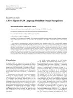
Figure 1: Ranking projection on the real line.
this is still too large to handle. Next, we present an efficient
approach that specifically handles the ranking problem with-
out exploding the size of the training data set.
3.3. Embedded space approach
In this section, we present a novel formulation that allows
one to map a ranking problem to a standard classification
problem without increasing the size of the data set. The em-
bedded space approach presented in this section is similar
in spirit to the model presented in [15], however as we will
see shortly in our model, the dimension of the new space
does not grow linearly as the one presented in their paper.
Figure 1 graphically depicts the ranking framework. The dis-
tance from the hyperplane h of a data point x
i
is mapped to
a one-dimensional space. In this space, θ
1
, , θ
K−1
are the
different thresholds against which the distance is compared.
Note that h
T
x
i
;forallx
i
having rank κ results in a range rep-

resented by its left end point θ
κ−1
and its right end point θ
κ
.
Define α
κ
= θ
κ+1
− θ
κ
;1≤ κ ≤ K − 1. For the data items
belonging to rank 1, there is no lower bound and for all the
data items belonging to rank K there is no upper bound. By
construction, it is easy to see that α
κ
> 0; for all κ. Note that
data point x
i
having rank κ>1 will satisfy (assuming α
0
= 0)
h
T
x
i
>θ
κ−1
,
h

T
x
i
+ α
κ−1
>θ
κ
,
h
T
x
i
+
K−2

r=κ−1
α
r
>θ
K−1
.
(2)
Similarly, for an example x
j
with rank κ<K(assuming θ
K
=
inf),
h
T

x
j
<θ
κ
,
h
T
x
j
+ α
κ
<θ
κ+1
,
h
T
x
j
+
K−2

r=κ
α
r
<θ
K−1
.
(3)
Based on this observation, define
h = [h, α

1
, α
2
, , α
K−2
]
and for an example x
j
with rank 1 <κ<K,definex
+
j
, x
−
j
as n + K − 2 dimensional vectors with
x
+
j
[l] =
⎧
⎪
⎪
⎨
⎪
⎪
⎩
x
j
[l], 1 ≤ l ≤ n,
0, n<l<n+ κ

− 1,
1, n + κ
− 1 ≤ l ≤ n + K − 2,
x
−
j
[l] =
⎧
⎪
⎪
⎨
⎪
⎪
⎩
x
j
[l], 1 ≤ l ≤ n,
0, n<l<n+ κ,
1, n + κ
≤ l ≤ n + K − 2.
(4)
For an example x
j
with rank κ = 1, we define only x
−
j
as
above and for an example with rank κ
= K,wedefineonly
x

+
j
again as above. This formulation assumes that θ
K−1
= 0.
It is easy to see that one can assume this without loss of
generality (by increasing the dimension of x by 1 one can
get around this). Once we have defined
x
+
j
, x
−
j
, the ranking
problem simply reduces to lear ning a classifier
h in n + K − 2
dimensional space such that
h
T
x
+
j
> 0andh
T
x
−
j
< 0. This
is a standard classification problem with at most 2m training

examples, half of which have label +1 (examples
x
+
j
) and the
rest have label
−1(examplesx
−
j
). Even though, the overall
dimension of the data points and the weight vector h is in-
creased by K
− 2, this representation limits the number of
training data points to be O(m). Note that although we have
slightly increased the dimension by K
− 2, the number of pa-
rameters that need to be learned is stil l the same (the classi-
fier and the thresholds). Interestingly, any linear classification
method can now be used to solve this problem. It is easy to
prove that if there exists a classifier that lear ns the above rule
with no error on the training data, then all the α
κ
sarealways
positive which is a requirement for the classification prob-
lem to be the same as the ranking problem. Next, we show
how one can use kernel classifiers (SVM) to solve the rank-
ing problem for data sets for which a linear ranker might not
exist.
3.4. Kernel classifiers: SVM
In many real world problems, it may not be possible to come

up with a linear function that would be powerful enough to
learn the ranking of the data. In such a scenario, standard
practice is to make use of kernels which allow nonlinear map-
ping of data. We will denote a kernel as K (
·, ·) = φ
T
(·)φ(·)
which corresponds to using the nonlinear mapping φ(
·)over
the original feature vector.
Solving ranking problems. For solving the ranking prob-
lem, we have proposed the mapping given in Section 3.3,one
has to be careful in using kernel classifiers with this mapping.
To see this, note that if x
j
has rank κ, then h
T
x
+
j
> 0 ⇒ h
T
x
j
>
θ
κ−1
; h
T
x

−
j
< 0 ⇒ h
T
x
j
>θ
κ
but K(h, x
+
j
) = φ
T
(h)φ(x
+
j
) >
0  φ
T
(h)φ(x
j
) >θ
κ−1
. This is again because of the non-
linearity of the mapping φ(
·). However, one can ag ain get
around this problem by defining a new kernel function. For
a kernel function K and the corresponding mapping φ(
·),
let us define a new kernel function

K and with the corre-
sponding mapping
φ(·)as
φ(x) =

φ(x), x[n +1:n + K − 2]

,
φ(h) =

φ(h), h[n +1:n + K − 2]

.
(5)
Note that, only the first n dimensions of
x corresponding to x
are projected to a higher dimensional space. The new kernel
function can hence be decomposed into sum of two kernel
functions where the first term is obtained by evaluation of
kernel over the first n dimensions of the vector and second
Mithun Das Gupta et al. 5
term is obtained by evaluating a linear kernel over the re-
maining dimensions,
K

x
i
, x
j


=
K

x
i
, x
j

+ x
i
[n +1:n + K − 2]
T
x
j
[n +1:n + K − 2].
(6)
However, when using the SVM algorithm with kernels, one
has to be careful while working in the embedded space.
Learning algorithms typically minimize the norm
h and
not
h as should have been the case. In the next section, we
introduce the problem of ordinal regression and show how
onecangetaroundthisproblem.
3.5. Reduction to ordinal regression
In this section, we show how one can actually get around the
problem of minimizing
h as against minimizing h.We
want to solve the following problem
min

1
2
h
2
,subjecttoy
+/−
j

h
T
x
+/−
j
+ b

> 0. (7)
The inequality in the above formulation for x
j
with rank y
j
can be written as,
−b −
n+k−2

l=n+1
h(l)x
−
j
(l) = θ
y

j
>h
T
x
j
> −b −
n+k−2

l=n+1
h(l)x
+
j
(l) = θ
y
j
−1
.
(8)
In this analysis, we will assume that with respect to threshold
θ
κ
’s, there is a margin of at least  such that for any data point
x
j
with corresponding rank y
j
,wehave
θ
y
j

−1
+  <h
T
x
j
,1<y
j
≤ K. (9)
Now, the problem given in (7) can be reframed as
min
1
2
h
2
,subjecttoh
T
x
j
<θ
y
j
, ∀1 ≤ y
j
<K
h
T
x
j
>θ
y

j
−1
+ ;1<yj≤ K.
(10)
This leads to the following Lagr ange formulation,
L
P
=
1
2
h
2
+
m−m
K

j=1
γ
+
j

h
T
x
j
− θ
y
j

+

m

j=m
1
+1
γ
−
j

θ
y
j
−1
+  − h
T
x
j

−

j
γ
+
j
−

j
γ
−
j

,
(11)
where m
κ
refers to number of elements having rank κ.The
ranker h is obtained by minimizing the above cost function
under the positivity constraints for γ
+
j
and γ
−
j
.Dualformu-
lation L
d
of the above problem can be obtained by following
the steps as in [16],
L
d
=−
1
2
n

i=1
n

j=1

γ

−
i
−γ
+
i

γ
−
j
−γ
+
j

K

x
i
, x
j

−

j
γ
+
j
−

j
γ

−
j
(12)
with constraints
m
κ

p=m
κ−1
+1
γ
+
p
=
m
κ+1

p=m
κ
+1
γ
−
p
, ∀κ ∈ [2, K − 1]. (13)
We have introduced γ
+
l
, γ
−
m

∀l ∈ [n
K−1
+1,n
K
]andm ∈
[1, n] for simplicity of notation. It is interesting to note that
(12) has the same form as a regression problem. The value
of θ
κ
’s is obtained using Karush-Kuhn-Tucker (KKT) condi-
tions.
4. SUPER-RESOLUTION USING MOTION ESTIMATION
In this section, we elaborate on the standard technique [17]
that is used for video super-resolution by accounting for mo-
tion estimation. The outline of the super-resolution tech-
nique is as follows.
(1) Bilinearly interpolate the frames to double their origi-
nal size.
(2) Warp (t
− n/2) to (t + n/2) frames onto the reference
frame t. This is one of the most important steps since
it generates the extra information needed for super-
resolving the frames. The quality of the super-resolved
frames depends on the accuracy of the image align-
ment techniques. A review of the different methods of
performing this step is given in [18, 19].
(3) Obtain a robust estimate for the tth frame. The way
in which the extra information is combined to pro-
duce the frames plays an important role in determin-
ing their quality. Simple techniques like averaging or

median operations to more complex techniques like
covariance intersection can all be employed in this
step. A few of the techniques for information fusion
are [20–22].
(4) Iterate over all the frames (excluding the boundary
frames).
(5) Repeat steps 2–4 until the estimates converge.
(6) Perform an optional deblurring operation on all the
frames.
In this work, we follow the guidelines introducing our own
algorithmic modules at appropriate places. For image regis-
tration and warping we use the hierarchical Lucas-Kanade
method [1] as used in the original work by Baker and Kanade
[17]. We use image patches of size 4
×4 for all the exper iments
reported in this work. This particular size was found to be
agoodtradeoff between the gain attained by encoding in-
formation more than that contained by individual pixels and
the smoothness introduced due to the patch size. As shown in
some of our experiments, the subpixel shifts are still present
after integer alignment and it is at this juncture that we per-
form our learning-based subpixel shift estimation algorithm.
The details of our algorithm are provided in Section 5.For
obtaining the robust estimate of the tth frame, we note that
there is a tradeoff between the simplicity of the technique and
the time taken for estimation. We employ simple techniques
like mean or median and find that the mean works quite
well for the results reported in this work. As pointed in the
original work by Baker and Kanade [17], simple mean works
6 EURASIP Journal on Advances in Signal Processing

comparably against other complicated methods, and hence
keeping the huge amount of video data in view, we adopt the
simple mean as a method to combine the multiple frames.
One point to note is that the 5th step in the algorithm which
is essentially iterating over the whole algorithm is avoided for
speed-up issues. All the results reported in this work are run
just for one iteration. Also the last step (6) has been avoided
in all our experiments. We take the liberty of omitting the last
step from all our results since this step is independent of the
algorithm used for the previous steps, and this work is prin-
cipally focussed on performing the shift estimation and not
on spatial domain deblurring techniques.
5. SUBPIXEL SHIFT ESTIMATION
Subpixel shift estimation involves identifying the shift in the
x and y directions between two patches wherein, we assume
that they have already been aligned in such a way that there
are no integer shifts between them. Traditionally, this prob-
lem has been solved using resolution pyramids in which the
subpixel shift problem is posed as an integer shift problem
in higher resolution. However, such a technique is limited
by the interpolation algorithm used for increasing the res-
olution. In this work, we adopt a learning strategy, namely,
the ranking framework discussed earlier for estimating the
subpixel shifts without increasing resolution. We note that
the notion of preference modeled by the ranking framework,
corresponds to the subpixel shift between two patches, say
in the x direction. Consider three patches denoted by p
1
, p
2

,
and p
3
and let the shift between p
2
and p
1
be a quarter pixel
shift and the shift between p
3
and p
1
be a half a pixel shift
in the x direction. The ranking framework accounts for the
ordering information, that is, p
1
is closer to p
2
than p
3
.Such
ordering information is not captured if we use a multiclass
classifier. The estimation problem becomes unrealistic when
posed as a regression problem because it imposes a metric on
the ranker output.
5.1. Polar coordinates
The subpixel shift estimation problem involves estimating
two different rankers which capture the shifts in the x and
y directions. However, we note that the two ranking prob-
lems are interrelated and treating them independently results

in bad empirical performance. Hence, we decouple the rela-
tion present in the Euclidean setting to an extent by posing
the shift estimation problem in the polar domain which cor-
responds to estimating the shift in the radial direction and
angular direction. In the radial direction, the learning prob-
lem falls under the category of the ranking formulation elab-
orated in Section 1. However, estimating shifts in the angular
direction leads to a different formulation that we term cir-
cular ordinality. Such a behavior arises naturally because of
the equivalence of an angular shift of 0 and 2π. Modeling
such behavior explicitly needs defining the notion of an an-
gular margin introducing nonlinearities in the cost function
which is hard to optimize. We overcome the above problem,
by a two step algorithm. The first step involves a classifier that
(a) (b)
(c) (d)
(e) (f)
(g) (h)
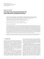
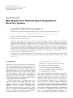
Figure 2: Image super-resolution. For each class, clockwise from
top left: (a), (e) original image, (b), (f) quarter pixel accuracy, (d),
(h) integer-pixel accuracy, (c), (g) half-pixel accuracy.
identifies the angular shift between two patches as either be-
ing in the upper half space (which corresponds to an angular
shift of 0
− π) or in the lower half space (which corresponds
to an angular shift of π
− 2π).Thesecondstepinvolvesiden-
tifying the angular shift in the relevant half space which can
be solved using the r a nking framework. In this work, we dis-
cretize the angular space uniformly into eight segments.

5.2. Regression coefficients as features
An important component of modeling is to identify/
construct features/attributes that efficiently represent the in-
put space in an informative way such that they aid in solv-
ing the learning problem well. Another novelty of this work
is a set of novel features for representing patch pairs. Con-
sider two patches p
i
and p
j
, where we denote the pixels in
the patches as p
ik
, and let there be P pixels in each patch.
Mithun Das Gupta et al. 7
(a) (b) (c) (d)
140120100806040200
0
20
40
60
80
100
120
140
(e)
140120100806040200−20
0
20
40

60
80
100
120
140
(f)
140120100806040200
0
20
40
60
80
100
120
140
(g)
140120100806040200
0
20
40
60
80
100
120
140
(h)
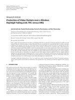
Figure 3: Top row: frames from the video. Bottom row: scaled flow vectors. Green: Lucas-Kanade. Red: our method.
We denote the set of adjacent neighbors of pixel location k as
N (k). We exploit the nature of subpixel shifts to model every
nonboundary pixel in the patch p

jk
, as a linear combination
of the pixels p
il
in the patch p
i
where l ∈{N (k) ∪ k}.The
above step results in a set of linear equations given by
p
jk
= w
T
ij
p
il
, l ∈

N (k) ∪ k

, (14)
where w
ij
represents the weight vector and k indicates one
of the nonboundary pixels in the patch p
j
. Further, we note
that the weight vector is invariant of k. We solve the above
linear regression problem in a least mean square error sense
to obtain the regression coefficients vector w
ij

. These regres-
sion coefficients are used to represent the patch pair p
i
and p
j
.
Higher order models can be used to model the patch depen-
dencies. Potential candidates to replace the linear predictors
can be median filter-based predictors [23] or hybrid filters
[24].
6. EXPERIMENTAL RESULTS
The experiments that we performed to demonstrate the ap-
plicability of our approach can be broadly classified into two
categories. The first experiment involves estimating global
motion for static images where the motion is generated ex-
clusively by camera motion and the scene is assumed to be
fixed. We estimate the amount of subpixel shift within con-
secutive frames and project the frames onto a higher resolu-
tion grid by accounting for the subpixel shifts. The unknown
pixels on the grid are then interpolated to generate high-
resolution images. In the second experiment, we demon-
strate the applicability of our approach on video frames
which have a moving foreground object and varying local
motion across different parts of the frame. We use subpixel
alignment techniques to generate the super-resolved video as
elaborated in Section 4.
6.1. Global subpixel motion
In this subsection, we investigate image super-resolution
with global subpixel shift estimation in which we syntheti-
cally generate the images by simulating camera shift against

a static backg round. We test our method for 3 different cat-
egories of images, namely, cars, license plates, and human
subjects. The training data used to learn the radial direc-
tion ranker and the classifier and ranker for angular direc-
tion estimation includes a mix of images belonging to differ-
ent categories from the Corel data set. The technique of es-
timating subpixel shifts is then used to perform static image
super-resolution. We used the traditional spatial alignment
method, wherein multiple low-resolution images are aligned
on a higher resolution grid. The unknown pixels remain-
ing on the grid are generated by bicubic interpolation. Since
the resolution improvement quality depends on the num-
ber of grid locations that can be filled accurately, without
interpolation, subpixel accuracies perform significantly bet-
ter than accounting for pure integer shifts. Also, the higher
the resolution of the subpixel estimation is the better the
results would be. We perform these experiments for the 3
classes of images mentioned above. The results are shown
in (Figure 2). Clearly, our method (quarter pixel accuracy)
and half-pixel accuracy are better than integer pixel accuracy.
Note the edges of the car bonnet or the edges of the digits in
the plate.
8 EURASIP Journal on Advances in Signal Processing
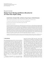
(a) (b) (c)
Figure 4: Left to right: (a) original scaled frame, (b) bicubic interpolation, (c) our method.
6.2. Local subpixel motion
In this subsection we report video super-resolution results by
estimating subpixel shifts of face videos. All the video are shot
with a Canon SD 450 camera. The frames are downsampled
to create the low-resolution inputs to our system.

In the first set of experiments, we verify the claim that
subpixel shifts still remain intact even after the frames have
been stabilized with respect to their temporal neighbors. For
this experiment, we took a video of a walking person and sta-
bilized the video using the algorithm proposed in [25, 26].
We use feature tracking to obtain the flow vectors and then
use our method to obtain the subpixel shifts in addition to
the flow vectors. We use Lucas-Kanade [1] to obtain the op-
tical flow vectors. The results are shown in Figure 3.
The final set of results show sequence of frames from
a face video. Each frame has been super-resolved using
the approach elaborated in Section 4.Wecompareourre-
sults against bicubic interpolation of the frames as shown
in Figure 4. Note that we do not perform the addition de-
blurring step which is commonly performed in other video
super-resolution algorithms. The results clearly indicate the
enhancement gain while performing motion and subpixel
shift estimation.
7. CONCLUSION AND FUTURE WORK
We have presented a learning-based algorithm for estimating
subpixel shifts in a patch based setting. The learning based
algorithm falls under the class of ranking problems in which
the ordering of the class labels is explicitly accounted for
which results in better performance over standard classifica-
tion and regression approaches. The ranking approach for
subpixel shift estimation is used to perform super-resolution
of images which have undergone a global subpixel shift and
enhancement of video frames which have undergone both
integer and subpixel shifts.
As mentioned earlier, higher order nonlinear models for

patch dependencies can be used to generate the features for
the determination of the azimuth angle. In the future, we
plan to use the subpixel shift estimation approach for other
applications, namely, motion tracking, layered motion, mo-
saic construction, medical image registration, and face cod-
ing. In the local subpixel shift estimation scenario, further
super-resolution can be performed by aligning pixels in a
higher-dimensional grid.
ACKNOWLEDGMENT
This work was supported in part by Disruptive Technology
Office (DTO) under Contract NBCHC060160.
REFERENCES
[1] B. Lucas and T. Kanade, “An iterative image registr ation tech-
nique with an application to stereo vision,” in Proceedings
of the 7th International Joint Conference on Artificial Intelli-
gence (IJCAI ’81), pp. 674–679, Vancouver, BC, Canada, Au-
gust 1981.
[2] J. K. Aggarwal and N. Nandhakumar, “On the computation of
motion from sequences of images—a review,” Proceedings of
the IEEE, vol. 76, no. 8, pp. 917–935, 1988.
[3] A. Mitiche and P. Bouthemy, “Computation and analysis of
image motion: a synopsis of current problems and methods,”
International Journal of Computer Vision, vol. 19, no. 1, pp. 29–
55, 1996.
[4] H H. Nagel, “Image sequence evaluation: 30 years and still
going strong,” in Proceedings of the 15th International Confer-
ence on Pattern Recognition (ICPR ’00), vol. 1, pp. 149–158,
Barcelona, Spain, September 2000.
[5] S. Rajaram, A. Garg, X. S. Zhou, and T. S. Huang, “Clas-
sification approach towards ranking and sorting problems,”

in Proceedings of the 14th European Conference on Machine
Learning (ECML ’03), pp. 301–312, Cavtat-Dubrovnik, Croa-
tia, September 2003.
[6] M C. Chiang and T. Boult, “Efficient image warping and
super-resolution,” in Proceedings of the 3rd Workshop on Appli-
cations of Computer Vision (WACV ’96), pp. 56–61, Sarasota,
Fla, USA, December 1996.
[7] F. Dellaert, S. Thrun, and C. Thorpe, “Jacobian images of
super-resolved texture maps for model-based motion estima-
tion and tracking,” in Proceedings of the 4th IEEE Workshop on
Applications of Computer Vision (WACV ’98), pp. 2–7, Prince-
ton, NJ, USA, October 1998.
Mithun Das Gupta et al. 9
[8] M. Elad and A. Feuer, “Super-resolution restoration of an im-
age sequence: adaptive filtering approach,” IEEE Transactions
on Image Processing, vol. 8, no. 3, pp. 387–395, 1999.
[9] R. C. Hardie, K. J. Barnard, and E. E. Armstrong, “Joint MAP
registration and high-resolution image estimation using a se-
quence of undersampled images,” IEEE Transactions on Image
Processing, vol. 6, no. 12, pp. 1621–1633, 1997.
[10] A. J. Patti, M. I. Sezan, and A. M. Tekalp, “Super-resolution
video reconstruction with arbitrary sampling lattices and
nonzero aperture time,” IEEE Transactions on Image Process-
ing, vol. 6, no. 8, pp. 1064–1076, 1997.
[11] T. S. Huang and R. Tsai, “Multi-frame image restoration and
registration,” in Advances in Computer Vision and Image Pro-
cessing, T. S. Huang, Ed., vol. 1, pp. 317–339, JAI Press, Green-
wich, Conn, USA, 1984.
[12] S. P. Kim, N. K. Bose, and H. M. Valenzuela, “Recursive recon-
struction of high resolution image from noisy undersampled

multiframes,” IEEE Transactions on Acoustics, Speech, and Sig-
nal Processing, vol. 38, no. 6, pp. 1013–1027, 1990.
[13] W. W. Cohen, R. E. Schapire, and Y. Singer, “Learning to order
things,” Journal of Artificial Intelligence Research, vol. 10, pp.
243–270, 1999.
[14] R. Herbrich, T. Graepel, and K. Obermayer, “Large margin
rank boundaries for ordinal regression,” in Advances in Large
Margin Classifiers, pp. 115–132, MIT Press, Cambridge, Mass,
USA, 2000.
[15] D. Roth, S. Har-Paled, and D. Zimak, “Constraint classifica-
tion: a new approach to multiclass classification,” in Proceed-
ings of the 13th Interntional Conference on Algorithmic Learning
Theory (ALT ’02), pp. 365–379, L
¨
ubeck, Germany, November
2002.
[16] A. Smola and B. Schlkopf, “A tutorial on support vector re-
gression,” Tech. Rep. NC2-TR-1998-030, Neural and Compu-
tational Learning 2 (NeuroCOLT2), London, UK, 1998.
[17] S. Baker and T. Kanade, “Super-resolution optical flow,” Tech.
Rep. CMU-RI-TR-99-36, Carnegie Mellon University, Pitts-
burgh, Pa, USA, 1999.
[18] S. Baker and I. Matthews, “Lucas-kanade 20 years on: a uni-
fying framework,” International Journal of Computer Vision,
vol. 56, no. 3, pp. 221–255, 2004.
[19] G. Wolberg, Digital Image Warping, IEEE Computer Society
Press, Los Alamitos, Calif, USA, 1992.
[20] X. Li, Y. Zhu, and C. Han, “Unified optimal linear estimation
fusion—I: unified models and fusion rules,” in Proceedings of
the 3rd International Conference on Information Fusion (FU-

SION ’00), vol. 1, pp. 10–17, Paris, France, July 2000.
[21] S. Julier and J. Uhlmann, “A non-divergent estimation algo-
rithm in the presence of unknown correlations,” in Proceedings
of the IEEE American Control Conference (ACC ’97), vol. 4, pp.
2369–2373, Alberquerque, NM, USA, June 1997.
[22] D. Comaniciu, “Nonparametric information fusion for mo-
tion estimation,” in Proceedings of the IEEE Computer Society
Conference on Computer Vision and Pattern Recognition (CVPR
’03), vol. 1, pp. 59–66, Madison, Wis, USA, June 2003.
[23] T. C. Aysal and K. E. Barner, “Quadratic weighted median fil-
ters for edge enhancement of noisy images,” IEEE Transactions
on Image Processing, vol. 15, no. 11, pp. 3294–3310, 2006.
[24] T. C. Aysal and K. E. Barner, “Hybrid polynomial filters for
Gaussian and non-Gaussian noise environments,” IEEE Trans-
actions on Signal Processing, vol. 54, no. 12, pp. 4644–4661,
2006.
[25] N. Petrovic, N. Jojic, and T. S. Huang, “Hierarchical video
clustering,” in Proceedings of the 6th IEEE Workshop on Multi-
media Signal Processing (MMSP ’04), pp. 423–426, Siena, Italy,
September 2004.
[26] N.Jojic,N.Petrovic,B.J.Frey,andT.S.Huang,“Transformed
hidden Markov models: estimating mixture models of images
and inferring spatial transformations in video sequences,” in
Proceedings of the IEEE Computer Society Conference on Com-
puter Vision and Pattern Recognition (CVPR ’00), vol. 2, pp.
26–33, Hilton Head, SC, USA, June 2000.
Mithun Das Gupta received his B.S. de-
gree in instrumentation engineering from
Indian Institute of Technology, Kharag-
pur in 2001, and his M.S. degree in elec-

trical engineering from University of Illi-
nois at Urbana Champaign in 2003. He
is currently pursuing his Ph.D. degree un-
der the guidance of Professor Thomas S.
Huang at the University of Illinois at Ur-
bana Champaign. His research interests in-
clude learning-based methods for image and video understanding
and enhancement.
Shyamsundar Rajaram received the B.S.
degree in electrical engineering from the
University of Madras, India, in 2000, and
the M.S. degree in electrical engineering
from the University of Illinois at Chicago
in 2002. He is currently working on his
Ph.D. degree at University of Illinois at Ur-
bana, Champaign under Professor Thomas
S. Huang. He has published several papers
in the field of machine learning and its ap-
plications in signal processing, computer vision, information re-
trieval, and other domains.
Thomas S. Huang received his B.S. degree
in electrical engineering from National Tai-
wan University, Taipei, Taiwan, China, and
his M.S. and Sc.D. degrees in electrical en-
gineering from the Massachusetts Institute
of Technology, Cambridge, Mass. He was on
the faculty of the Department of Electrical
Engineering at MIT from 1963 to 1973, and
on the faculty of the School of Electrical En-
gineering and Director of its Laboratory for

Information and Signal Processing at Purdue University from 1973
to 1980. In 1980, he joined the University of Illinois at Urbana-
Champaign, where he is now William L. Everitt Distinguished Pro-
fessor of Electrical and Computer Engineering, and Research Pro-
fessor at the Coordinated Science Laboratory, and Head of the Im-
age Formation and Processing Group at the Beckman Institute for
Advanced Science and Technology and Cochair of the Institute’s
major research theme of human-computer intelligent interaction.
Nemanja Petrovic received his Ph.D. de-
gree from University of Illinois in 2004. He
is currently a member of research staff at
Google Inc., New York. His professional in-
terests are computer vision and machine
learning. Dr. Petrovic has published more
than 20 papers in the fields of graphi-
cal models, video understanding, and data
clustering and image enhancement.