Báo cáo hóa học: " Research Article Distortion-Free 1-Bit PWM Coding for Digital Audio Signals" pdf
Bạn đang xem bản rút gọn của tài liệu. Xem và tải ngay bản đầy đủ của tài liệu tại đây (1.08 MB, 12 trang )
Hindawi Publishing Corporation
EURASIP Journal on Advances in Signal Processing
Volume 2007, Article ID 94386, 12 pages
doi:10.1155/2007/94386
Research Article
Distortion-Free 1-Bit PWM Coding for Digital Audio Signals
Andreas Floros
1
and John Mourjopoulos
2
1
Department of Computer Science, Ionian University, Plateia Tsirigoti 7, 49 100 Corfu, Greece
2
Audio Technolog y Group, Department of Electrical and Computer Engineer ing, University of Patras, 265 00 Rio Patras, Greece
Received 15 June 2006; Revised 1 December 2006; Accepted 13 March 2007
Recommended by Sven Nordholm
Although uniformly sampled pulse width modulation (UPWM) represents a very efficient digital audio coding scheme for digital-
to-analog conversion and full-digital amplification, it suffers from strong harmonic distortions, as opposed to benign non-
harmonic artifacts present in analog PWM (naturally sampled PWM, NPWM). Complete elimination of these distortions usually
requires excessive oversampling of the source PCM audio signal, which results to impractical realizations of digital PWM systems.
In this paper, a description of digital PWM distortion generation mechanism is given and a novel principle for their minimization
is proposed, based on a process having some similarity to the dithering principle employed in multibit signal quantization. This
conditioning signal is termed “jither” and it can be applied either in the PCM amplitude or the PWM time domain. It is shown that
the proposed method achieves significant decrement of the harmonic distortions, rendering digital PWM performance equivalent
to that of source PCM audio, for mild oversampling (e.g.,
×4) resulting to typical PWM clock rates of 90 MHz.
Copyright © 2007 A. Floros and J. Mourjopoulos. This is an open access article distributed under the Creative Commons
Attribution License, which permits unrestricted use, distribution, and reproduction in any medium, provided the original work is
properly cited.
1. INTRODUCTION
Over the last decades, the use of 1-bit audio signals has
emerged as an attractive practical alternative to multibit
pulse code modulation (PCM) audio, which up to now was
considered as the de facto format for the representation of
such data. The advantages of a pulse-stream representation
for digital audio originate from the simpler hardware imple-
mentations with respect to the required audio performance.
For example, analog-to-digital (ADC) and digital-to-analog
(DAC) conversion systems with the increased requirements
imposed in dynamic range and bandwidth can be efficiently
implemented using 1-bit digital storage formats (i.e., in the
form of direct stream digital—DSD [1],whichisbasedupon
sigma-delta modulation—SDM [2]).
Similarly, conversion of audio to 1-bit pulse width mod-
ulation (PWM) streams introduces comparable practical im-
plementation advantages for the realization of DACs [3]
and other components in the audio chain, especially all-
digital amplifiers, since the PWM pulse-stream can be di-
rectly amplified using power switch transistors [4]. Theo-
retically, any switching power stage has 100% efficiency. In
practice, no ideal power switch exists and such implemen-
tations result into an amount of power loss taking place
when the power switches cross their linear range [5]. Hence,
although SDM requires no linearization for achieving ac-
ceptable distortion levels, PWM audio coding represents a
more attractive dig ital amplification format, since it incor-
porates lower number of power switch transitions. More
specifically, as it will be discussed in the following section,
the 1-bit PWM stream representation requires two differ-
ent clocks: the sampling frequency f
s
that equals to the
PWM pulse transitions repetition and a much higher clock
f
p
that determines the exact time instances of these tran-
sitions. On the contrary, for SDM both the sampling and
the pulse repetition rates are the same with a value in the
range of 2.8 MHz. This increased pulse repetition rate im-
ply higher power dissipation and lower power efficiency, due
to the very frequent transition of the MOSFET switches im-
plementing the final output stage over their linear operating
region [6]. Further m ore, PWM coding also overcomes po-
tential problems associated with SDM audio coding, such as
out-of-band noise amplification, zero-level input signal idle
tones and limit cycles responsible for audible baseband tones
[7, 8].
Although many all-digital amplification commercial sys-
tems are now appearing, the theoretical implications of us-
ing such 1-bit data are not very well understood and usu-
ally these systems employ practical “rule of thumb” solutions
to suppress unwanted side effects and distortions generated
2 EURASIP Journal on Advances in Signal Processing
Analog carrier
signal generator
f
s
Analog
source
Discrete-time
carrier signal
generator
N,
f
s
f
s
Quantizer
Q[]
f
s
= 2 f
s
Quantizer
Q[]
Discrete-time domain
Comparator
NPWM
UPWM
A-UPWM
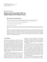
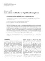
Figure 1: Alternative PWM modulation schemes.
from the conversion of the better understood multibit PCM
format into 1-bit signal [9].
Focusing on PWM conversion, the inherently non-
linear nature of this process introduces harmonic and non-
harmonic distortions [10], which render the audio perfor-
mance unsuitable for most applications. Although some dis-
tortion compensating strategies have been proposed [11, 12],
none of them has achieved complete elimination of PWM
distortions and most implementations rely on significant in-
crease of the modulators’ switching frequency. However, this
approach proportionally increases the system complexity, in-
troduces electromagnetic interference problems, and negates
the basic PWM advantage over SDM, as it decreases the over-
all digital amplification efficiency, due to the increment of the
PWM pulse repetition frequency [13].
The work here attempts to overcome the above problems
and to improve understanding of digital audio PWM. It in-
troduces a novel analytic approach, which allows exact de-
scription of the PWM pulse stream as well as prediction and
suppression of distortion a rtifacts of such audio signals with-
out excessive increment of the pulse repetition frequency,
starting from the following initial assumptions.
(a) The dig ital audio source will be in the widely em-
ployed PCM format (typically sampled at f
s
= 44.1 kHz and
quantized using N
= 16 bit).
(b) The case of regularly sampled (discrete-time) PWM
conversion will be examined (uniformly sampled PWM,
UPWM), appropriate for mapping from the sampled PCM
audio data.
(c) The UPWM format can be related to the inherently
analog naturally sampled PWM (NPWM), w hich tradition-
ally has been analyzed and employed in many communica-
tion applications [14]. Due to the asymmetric positioning of
the NPWM pulse edges, the asymmetric uniformly sampled
PWM (A-UPWM) must be also examined [15, 16], as shown
in Figure 1.
(d) As it is known, NPWM generates only nonharmonic
type distortions, which can be easily eliminated from the au-
dio band by appropriately increasing the modulation switch-
ing frequency [17]. However, UPWM and A-UPWM being
discrete-time processes, it is also well known to generate ad-
ditional harmonic distortions [10, 18 ]. Furthermore, assum-
ing that the PCM audio data do not posses any form of dis-
tortions, it would be sensible to consider here conditions un-
der which the mapping error between PCM and A-UPWM
would be eliminated. Nevertheless, it is analytically shown
here (see the appendix) that this condition is only satisfied
for a full-scale DC signal, so that it will not be applicable
to any practical audio data. Therefore, the work here will be
mainly concerned with the minimization of errors between
NPWM and the equivalent A-UPWM conversion. It will be
shown that such an approach will also allow optimal map-
ping between the PCM and UPWM.
The work is organized as follows: in Section 2,anovel
analytic description of the A-UPWM and NPWM coding is
introduced. It is also shown (Section 3) that the A-UPWM-
induced harmonic distortions are generated due to the sam-
pling process applied during the PCM-to- A-UPWM map-
ping. Hence, a novel principle for minimizing such signal-
related distortions in 1-bit digital PWM signals is introduced
in Section 4, having some parallels to the dithering principle
employed for minimizing amplitude quantization artifacts in
multibit PCM conversion [19]. This principle can be also ex-
pressed as controlled jittering of the UPWM pulse transition
edges, and hence it is termed “jithering.” Section 5 presents
typical performance results of the proposed method, show-
ing that it achieves acceptable levels of signal-dependent
(harmonic) UPWM distortions under all practical condi-
tions.
2. PWM CONVERSION FUNDAMENTALS
Legacy PWM represents data as width-modulated pulses
generated by the comparison of the analog or digital audio
waveform with a periodic carrier signal of fundamental fre-
quency f
s
(Hz), as is shown in Figure 1. More specifically, the
switching instances of the PWM pulses are defined by the in-
tersection of the input signal and the carrier waveform. For
double-edged PWM considered here, the carrier should be
of triangular shape, while depending on the analog or digital
nature of the input, it should be an analog or a discrete-time
signal, respectively.
Assuming a PCM input signal, bounded in the range of
[0, S
max
], sampled at f
s
= 2 f
s
and quantized to N bit, the au-
dio information will be represented by 2
N
discrete amplitude
levels. In order to preserve this information after PWM con-
version, the PWM pulse stream should be also quantized in
the time domain with an equivalent resolution. Thus, within
each time interval T
s
= 1/f
s
,2
N
different equally spaced in-
tersection values should be allowed between the car rier and
the digital input samples. Following this argument, the car-
rier waveform will be a discrete-time signal of sampling fre-
quency f
p
= 1/T
p
(Hz), where
T
p
=
T
s
2
2
N
− 1
=
T
s
2
N
− 1
,(1)
A. Floros and J. Mourjopoulos 3
CR(t)or
CR(m)
s(t)
(a)
s
q
(kT
s
) s
q
(kT
s
+ T
s
/2)
T
s
A-UPWM
k
(mT
p
)
m
lead,k
T
p
m
trail,k
T
p
A-UPWM
k+1
(mT
p
)
(b)
NPWM
k
(t)
t
trail,k
t
lead,k
NPWM
k+1
(t)
(c)
E
lead,k
E
trail,k
E
lead,k+1
E
trail,k+1
(d)
kT
s
(k +1)T
s
(k +2)T
s
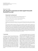
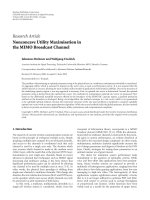
Figure 2: Typical audio waveforms: (a) analog/digital audio and modulation carrier (b) A-UPWM (c) NPWM (d) absolute A-UPWM to
NPWM difference.
and within the kth switching period T
s
it can be expressed as
CR
k
(m) =
⎧
⎪
⎪
⎪
⎪
⎪
⎪
⎪
⎪
⎪
⎪
⎪
⎪
⎪
⎪
⎨
⎪
⎪
⎪
⎪
⎪
⎪
⎪
⎪
⎪
⎪
⎪
⎪
⎪
⎪
⎩
−
S
max
m − 2k
2
N
− 1
2
N
− 1
+ S
max
,
for 2k
2
N
−1
≤
m≤(2k+1)
2
N
−1
,
S
max
m − 2k
2
N
− 1
2
N
− 1
− S
max
,
for
2k+1
2
N
−1
≤
m≤2(k+1)
2
N
−1
,
(2)
where m is the PWM time-domain discrete-time integer vari-
able defined for [0,
∞).
In such a case, the leading and trailing edges of the kth
PWM pulse (see Figure 2) will be defined at integer multiples
m
lead,k
and m
trail,k
of the period T
p
defined as
s
q
kT
s
= CR
k
m
lead,k
,
s
q
kT
s
+
T
s
2
=
CR
k
m
trail,k
,
(3)
where s
q
(kT
s
)ands
q
(kT
s
+T
s
/2) are the digital input samples.
Using (2)and(3), the leading and trailing edge instances of
the kth PWM pulse will be
m
lead,k
T
p
=
2k +1−
s
q
kT
s
S
max
2
N
− 1
T
p
=
2k +1−
s
q
kT
s
S
max
T
s
2
,
(4a)
m
trail,k
T
p
=
2k +1+
s
q
kT
s
+ T
s
/2
S
max
T
s
2
. (4b)
Assuming now a n analog input signal s(t), its intersec-
tion with the carrier signal can occur at any time instance
within each period T
s
, the carrier waveform of (2) being de-
fined also as an analog signal. Following a similar analysis to
the one performed for digital inputs, the two intersection in-
stances (one in each half of the period T
s
) between the signal
s(t) and the carrier CR
k
(t) will be given by the expressions
t
lead,k
=
T
s
2
2k +1−
s(t
lead,k
)
S
max
,
t
trail,k
=
T
s
2
2k +1+
s(t
trail,k
)
S
max
.
(5)
Due to the time irregularity of the input signal sampling
process perfor m ed at the time instances t
lead,k
and t
trail,k
, the
above process is called naturally sampled PWM (NPWM).
Each NPWM pulse within the kth switching period T
s
can
be expressed as
NPWM
k
(t) = A
u
t − t
lead,k
− u
t − t
trail,k
,(6)
4 EURASIP Journal on Advances in Signal Processing
where A is the amplitude of the NPWM pulses and u(t) the
analog-time step function defined as
u(t)
=
⎧
⎨
⎩
1, t ≥ 0,
0, otherwise.
(7)
On the other hand, in the case of digital input signals, the
regularly spaced sampling instances kT
s
and kT
s
+ T
s
/2gen-
erate the asymmetric uniformly sampled PWM ( A-UPWM)
expressed as
A
− UPWM
k
(m)
=A
u
m −
2k +1− a
q
kT
s
2
N
− 1
−
u
m −
2k +1+a
q
kT
s
+
T
s
2
2
N
− 1
,
(8)
where u(m) is the discrete-time step function and a
q
(kT
s
)
is the normalized input signal amplitude defined by the ra-
tio s
q
(kT
s
)/S
max
. Assuming that the sampling frequency f
s
of
the digital input data is equal to the carrier fundamental pe-
riod f
s
, then both the leading and trailing edges of the PWM
pulses will be modulated by a single quantized input signal
value s
q
(kT
s
). This produces the well-known case of the uni-
formly sampled PWM (UPWM), which is described in the
time domain by (8) by setting a
q
(kT
s
+ T
s
/2) = a
q
(kT
s
)[18].
3. UPWM-INDUCED DISTORTIONS
Let us now compare the time-domain waveforms of the
NPWM and A-UPWM streams, as described by (6)and(8).
Given that the amplitude of the PWM pulses in both modu-
lation schemes is kept constant (and equal to A) within each
switching interval, we can define their time-domain differ-
ence in terms of absolute time values (see Figure 2)as
E
k
= E
lead,k
+ E
trail,k
,(9)
where
E
lead,k
= A
t
lead,k
− m
lead,k
T
p
,
E
trail,k
= A
t
trail,k
− m
trail,k
T
p
.
(10)
Using the set of (4)and(5), the above expressions give
E
lead,k
=
AT
s
2S
max
s
q
kT
s
− s
t
lead,k
,
E
trail,k
=
AT
s
2S
max
s
t
trail,k
−
s
q
kT
s
+
T
s
2
.
(11)
Given that the error ε
l,k
and ε
t,k
generated by the ampli-
tude quantization of the discrete time values s(kT
s
)and
s(kT
s
+T
s
/2) to the digital samples s
q
(kT
s
)ands
q
(kT
s
+T
s
/2)
is expressed as [20]
ε
l,k
=s
kT
s
−
s
q
kT
s
,
ε
t,k
=s
kT
s
+
T
s
2
−
s
q
kT
s
+
T
s
2
,
(12)
where
− LSB /2 ≤ ε
l,k
≤ LSB /2and− LSB/2 ≤ ε
t,k
≤ LSB /2,
with LSB presenting the least significant bit of the input P CM
data, (11)give:
E
lead,k
=
AT
s
2S
max
s
kT
s
− s
t
lead,k
− ε
l,k
,
E
trail,k
=
AT
s
2S
max
s
t
trail,k
−
s
kT
s
+
T
s
2
+ ε
t,k
.
(13)
By observing the above e quations, it is obvious that the
time domain difference between A-UPWM and NPWM in
each switching period will be due to two independent but si-
multaneously acting mechanisms: (a) the amplitude-domain
quantization of the input signal affecting the A-UPWM con-
version, expressed by the quantization error terms ε
l,k
and
ε
t,k
, and (b) the difference of the sampling instances between
the NPWM (i.e., t
lead,k
and t
trail,k
) and A-UPWM (i.e., kT
s
and kT
s
+ T
s
/2).
Considering the first mechanism, it is clear that in the
case of NPWM modulation, the analog (and continuous) na-
ture of the input signal’s amplitude wil l result to similarly
continuous time variables t
lead,k
and t
trail,k
, which will define
the NPWM pulse transitions. On the contrary, in the case
of A-UPWM, the quantized (and discontinuous) nature of
the input signal amplitude will result to discrete time values
m
lead,k
T
p
and m
trail,k
T
p
which will define the exact positions
of the A-UPWM pulse edges in the time axis. Hence, given
that T
p
represents the shorter A-UPWM pulse possible time
duration that corresponds to the minimum amplitude value
defined for PCM coding (i.e., the PCM least significant bit—
LSB), this interval can be termed as the least significant time
transition (LST) for the A-UPWM coding.
Moreover, as can be observed from (11), the mapping of
the amplitude quantization of the PCM signals s
q
(kT
s
)and
s
q
(kT
s
+T
s
/2) into discrete time variables has the typical form
of the well-known amplitude quantization. As it is known,
the error generated by such quantization, under certain as-
sumptions (which are generally satisfied by any digital audio
signal), will produce noise that has broadband nature and
with amplitude roughly equal to 6N [21]. Hence when map-
ping N-bit quantized values into the discrete time domain as
given by (1), under the same assumptions, the signal noise
floor level will not be affected.
Considering now the second mechanism, it is clear that
in the case of the NPWM, the pulse edges coincide with the
time instances at which the input signal is sampled and fed to
the NPWM modulator and this natural (i.e., continuous and
nonregular) sampling wil l result to a finely sampled signal
which in effect will generate only the wel l-known intermod-
ulation products [10]atfrequencies
f
= ax
2 f
s
−
b × f
in
, (14)
where a, b are nonzero integers and f
in
is the input signal f re-
quency. On the contrary, in the case of A-UPWM, the sam-
pling of the discrete PCM data at regular time instances will
result to an accumulated shifting of the PWM-pulse edges
(with respect to the NPWM sampling), which generates a
signal-dependent FM-type modulation [15], resulting to the
A. Floros and J. Mourjopoulos 5
rise of the well-known harmonic distortion. It should be also
noted that the amplitude of the intermodulation and har-
monic distortion artifacts is not affected in any way by the
quantization resolution employed. Nevertheless, the reduc-
tion of the quantization resolution N, can render these dis-
tortion artifacts nonaudible, due to masking by the increased
noise floor level [22].
4. A-UPWM DISTORTION MINIMIZATION
Following the analysis in the previous section, a possible A-
UPWM harmonic distortion suppression scheme is to ap-
proximate the A-UPWM sampling instances with those de-
rived using the NPWM coding scheme. This approximation
can be performed by minimizing the time-domain difference
E
k
of A-UPWM and NPWM expressed using (9)and(10)as
E
k
= A
t
lead,k
− m
lead,k
T
p
+
t
trail,k
− m
trail,k
T
p
, (15)
or equivalently, using the set of (11):
E
k
=
AT
s
2S
max
s
q
kT
s
−s
t
lead,k
+
s
t
trail,k
−s
q
kT
s
+
T
s
2
.
(16)
Obviously, the minimization of E
k
can be efficiently
achieved when the sampling interval T
s
decreases, that is,
when using sufficiently high oversampling, typically by a fac-
tor o f
×64 [22]. In this case, the derived oversampled signal
better approximates its original analog equivalent, hence the
A-UPWM stream pulse transition instances are closer to the
NPWM pulse edges. However, in this case, (1) results into
extremely high PWM clock rates f
p
that are impossible to be
realized in prac tice.
Here, a novel solution is proposed, based on the follow-
ing two alternative strategies: (a) in the amplitude domain,
by proper modification of the amplitude of the input sam-
ples s
q
(kT
s
)ands
q
(kT
s
+ T
s
/2). This process is equivalent to
adding digital dither prior to A-UPWM conversion, or (b)
in the time domain, by proper displacement (jittering) of the
A-UPWM pulse edges.
Hence, the generic term “jither” can be employed to de-
scribe both minimization strategies [23]. Such minimiza-
tion will remove all harmonic artifacts without affecting the
nonharmonic distortions inherent to the “NPWM-like” na-
ture of the “jithered” A-UPWM, which however can be eas-
ily eliminated from the audio band by simply doubling the
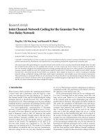
conversion switching frequency. Thus, the proposed PWM
distortion minimization method is based on the structure
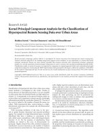
shown in Figure 3, having the following stages.
(i) A “jither” module, implemented in either the PCM-
amplitude or the PWM-time domain. This renders A-
UPWM equivalent to NPWM and removes all PWM-
induced harmonic distortions. Especially if UPWM conver-
sion is considered, (which is the typical case in digital audio
applications) an
×2 oversampling process must be also em-
ployed within this module in order to produce the A-UPWM
waveform which does not affect the final PWM rate.
PCM input
Optional
xR (e.g. R
= 4)
oversampling
Noise-shaping
Alternative A Alternative B
N
N
Quantizer
Jither module
Amplitude-
domain jithering
PCM-to-
A-UPWM mapper
PCM-to-UPWM
mapper
Time-
domain jithering
PWM 1-bit
output
PWM 1-bit
output
Figure 3: Block diagram of the proposed PWM correction chain.
(ii) An ×R oversampling stage (typically R = 2) which
will shift the NPWM-like nonharmonic intermodulation ar-
tifacts outside the audio band.
(iii) An optional input PCM amplitude quantizer stage
(e.g., from N
= 16 to N
= 8 bit), so that the final PWM
clock rates can be kept to desirable low values. More specif-
ically, according to (1), the PWM clock rate in the case of
N
= 16 bit equals to 5.7 GHz (11.5 GHz when ×2oversam-
pling is applied), which may prove to be prohibitive for prac-
tical implementations. For the reduction of these rates to fea-
sible values, the preconditioned samples must be requantized
to 8-bit prior to the PCM-to-A-UPWM mapping. However,
in this case, provided that the 8-bit resolution results into au-
dible quantization error levels and relative poor audio qual-
ity, this process must be combined with (a) oversampling in
the PCM domain (prior to the “jither” module) for reduc-
ing the overall quantization error level and (b) noise-shaping
techniques [24]foreffectively spreading the quantization er-
ror to less obtrusive (i.e., higher frequency) areas of the au-
dio spectrum using conventional FIR filters. As presented in
[22], a 3rd order noise shaper can significantly improve the
8-bit PCM-to-PWM mapping in terms of quantization noise
audibility.
In the following sections, a more detailed analysis of
the “jither” module in both amplitude and time domains is
given.
4.1. “Jither” addition in the amplitude domain
Let us assume that the input to an A-UPWM coder is a sig-
nal sampled at a rate 2 f
s
with resolution N bit, described by
the samples s
q
(kT
s
)ands
q
(kT
s
+ T
s
/2) in each T
s
interval.
The minimization of the NPWM and A-UPWM difference
E
k
expressed by (16) can be achieved by adding appropri-
ately evaluated N-bit quantized “jither” values g
lead
(kT
s
)and
g
trail
(kT
s
+ T
s
/2) to the corresponding input signal samples
s
q
(kT
s
)ands
q
(kT
s
+ T
s
/2) prior to A-UPWM conversion,
6 EURASIP Journal on Advances in Signal Processing
hence producing the “jithered” values s
q
(kT
s
)ands
q
(kT
s
+
T
s
/2) as
s
q
kT
s
=
s
q
kT
s
+ g
lead
kT
s
,
s
q
kT
s
+
T
s
2
=
s
q
kT
s
+
T
s
2
+ g
trail
kT
s
+
T
s
2
.
(17)
As previously mentioned, both g
lead
(kT
s
)andg
trail
(kT
s
+T
s
/2)
values are evaluated for concurrently minimizing both terms
E
lead,k
and E
trail,k
of the difference between NPWM and A-
UPWM. Considering constant sampling period (T
s
)values
and following (11), the above minimization is expressed as
s
q
kT
s
−
s
t
lead,k
≤
LSB
2
,
s
t
trail,k
− s
q
kT
s
+
T
s
2
≤
LSB
2
.
(18)
It should be noted that the NPWM and A-UPWM differ -
ence minimization is theoretically limited within the range
[
− LSB /2, LSB/2], due to the N-bit quantization of the digi-
tal samples s
q
(kT
s
)ands
q
(kT
s
+ T
s
/2).
4.2. “Jither” addition in the PWM time domain
Alternatively, the NPWM and A-UPWM difference mini-
mization expressed by (15) can be performed directly in the
PWM domain by “jittering” the leading and trailing edge
of the kth A-UPWM pulse by the quantities J
lead,k
T
p
and
J
trail,k
T
p
(sec), where J
lead,k
and J
trail,k
are integer indices ex-
pressing the time displacement of the PWM pulse edges as
multiples of the LST. In such a case, it is required that these
indices are calculated using the expressions
t
lead,k
− m
lead,k
T
p
≤
LST
2
,
t
trail,k
− m
trail,k
T
p
≤
LST
2
,
(19)
where the integer indices
m
lead,k
= m
lead,k
− J
lead,k
,
m
trail,k
= m
trail,k
+ J
trail,k
,
(20)
define the “jittered” positions of the A-UPWM pulse edges
as multiples of the PWM fundamental period T
p
. Again,
the above t ime-domain minimization of the NPWM and A-
UPWM pulse edges positions is theoretically limited within
the range [
− LST /2, LST/2] due to the N-bit quantization of
the PWM time domain.
4.3. “Jither” realization
Following the set of (18), the exact “jither” values in the am-
plitude domain can be calculated, provided that the input
sample values s(t
lead,k
)ands(t
trail,k
) are already known. The
same stands in the time-domain “jither” calculation, where
the sampling instances t
lead,k
and t
trail,k
were assumed to be
known in (19). However, this assumption is impractical in
the case of digital PWM conversion, as it requires the pres-
ence of the analog version of the input signal.
In order to overcome the above problem, a novel algo-
rithm was developed and is described in this par agraph for
providing a very close estimation of the above-unknown val-
ues. It should be noted that, although the following analysis
of the proposed algorithm focuses on time-domain “jither,” it
could be similarly described in the case of amplitude-domain
“jither” as well.
Using the set of (19) and taking into account (4a), the
proposed algorithm iteratively provides an estimation of the
kth PWM pulse leading edge time instance as
m
i+1
lead,k
=
2k +1−
s
m
i
lead,k
T
p
S
max
2
N
− 1
, (21)
where i is an integer that denotes the iteration index for the
current “jither” value estimation. Obviously, for i
= 0, the
value s(m
0
lead,k
T
p
)equalstos(kT
s
) and the resulting m
1
lead,k
T
p
value represents the leading edge instance of the legacy A-
UPWM described in Section 2. The above iterative process is
repeated until the following condition is validated:
m
i+1
lead,k
− m
i
lead,k
≤
D
τ
, (22)
where D
τ
is a positive nonzero integer that defines the
accuracy (i.e., the degree of approximation of the A-
UPWM and NPWM) as multiple of the LST, that is
[
−D
τ
(LST /2), D
τ
(LST /2)]. Clearly, when D
τ
= 1, the maxi-
mum theoretic approximation accuracy is achieved imposed
by (19), due to the time-domain quantization of the A-
UPWM pulse edges within the range [
− LST /2, LST/2]. As
it will be shown later, the highest this approximation accu-
racy is, the largest number of iterations is performed and the
corresponding computational load required for realizing the
A-UPWM and NPWM approximation is increased.
In (21) the input signal value s(m
i
lead,k
T
p
) must be also
calculated. For this reason, the original digital audio input is
oversampled prior to PWM conversion and the “jithering”
process, typically by a factor
×R
v
. As it will be show n later,
this oversampling process does not affect the final PWM rate
f
p
, hence it is termed here as “virtual” oversampling. After
virtual oversampling, in each input signal sampling period
T
s
, a total number of R
v
input signal values are available, de-
noted as s(kT
s
), s(kT
s
+ T
s,R
), , s(kT
s
+ rT
s,R
), , s(kT
s
+
(R
v
−1)T
s,R
)whereT
s,R
= T
s
/R
v
. During the ith iteration step
of (21), the samples s(kT
s
+ r
i
T
s,R
)ands(kT
s
+(r
i
+1)T
s,R
)
are selec ted which satisfy the equation
kT
s
+ r
i
T
s,R
≤ m
i
lead,k
T
p
≤ kT
s
+
r
i
+1
T
s,R
(23)
and these samples are employed for calculating the desired
signal value s(m
i
lead,k
T
p
) using linear approximation, that is,
s
m
i
lead,k
T
p
=
s
kT
s
+ r
i
T
s,R
+
s
kT
s
+
r
i
+1
T
s,R
−
s
kT
s
+ r
i
T
s,R
T
s,R
×
m
i
lead,k
T
p
−
kT
s
+ r
i
T
s,R
.
(24)
A. Floros and J. Mourjopoulos 7
Oversampling
(xR
v
)
s(kT
s
+ r
i
T
s,R
)
s(kT
s
+(r
i
+1)T
s,R
)
s(kT
s
)
PCM-to-
A-UPWM mapper
Time-domain
requantizer
m
i
lead,k
m
i
trail,k
m
lead,k
m
trail,k
m
i+1
lead,k
m
i+1
trail,k
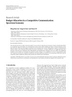
Figure 4: Block diagram of the proposed “jither” implementation
algorithm in the time domain.
The same calculations’ sequence is followed in the case of
trailing edge time instance using the equation
m
i+1
trail,k
=
2k +1+
s
m
i
trail,k
T
p
S
max
2
N
− 1
(25)
until
m
i+1
trail,k
− m
i
trail,k
≤
D
τ
. (26)
The above “jither” values estimation procedure is sum-
marized in Figure 4. The iteration path between the PCM-to-
A-UPWM mapper and the time-domain requantizer that re-
alizes (21)and(25) is followed until the conditions described
by (22)and(26) are reached. In this case, the algorithm out-
puts the values m
lead,k
and m
trail,k
which define the “jithered”
leading and trailing edges of each PWM pulse, respectively.
It should be also noted that, in the above analysis, the
PWM pulse repetition rate equals to f
s
(the digital input sig-
nal sampling frequency). Hence, although virtual oversam-
pling is employed, the final PWM clock rate is not propor-
tionally increased. Moreover, due to the time-domain re-
quantization stage which appeared in Figure 4, the optional
requantizer module which appeared in Figure 3 is not neces-
sary, as the appropriate selection of the D
τ
parameter value
results into the direct requantization of the input signal into
the time domain. For example, assuming that the or iginal bit
resolution of signal s(kT
s
)equalstoN,avalueD
τ
= 2
N
would result into requantization to (N-N
) bits, while for
D
τ
= 1(N
= 0), no requantization is performed.
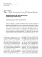
5. RESULTS AND IMPLEMENTATION
5.1. Harmonic distortion suppression
Figure 5 shows the 1-bit PWM spectrum in the case of a
full-scale (0 dB relative full scale, dB-FS) 5 kHz sinewave sig-
nal, originally sampled at f
s
= 44.1 kHz and quantized us-
ing 16 bit. When
×2 oversampling is applied on the input
data, the UPWM spectrum contains the well-know n even
and odd numbered harmonics. No intermodulation prod-
ucts are present due to the
×2 oversampling. Moreover, in
this case, as no requantization is applied, the noise floor level
110
Frequency (kHz)
120
90
60
30
0
120
90
60
30
0
120
90
60
30
0
Amplitude (dB-FS)
16-bit UPWM
R
= 2, f
p
= 11.56 GHz
16-bit jithered PWM
R
= 2, f
p
= 11.56 GHz
8-bit jithered PWM
R
= 4, f
p
= 89.96 MHz
SDM
Figure 5: “Jither” effect on the final PWM spectrum in the case of
5 kHz, 0 dB-FS sinewave signal ( f
s
= 44.1kHz).
is equivalent to a 16-bit PCM signal and the final PWM clock
rate equals to f
p
= 11.56 GHz. Under the same clock rates,
when “jithering” is applied (using R
v
= 32 for optimized per-
formance as described in the following section), all harmonic
intermodulation products are eliminated.
Although the above example clearly demonstrates the ef-
ficiency of the proposed “jithering” technique, the excessive
final PWM clock rate value debars any practical realization
of such a system. However, if time-domain requantization
to N
= 8 bit (i.e., D
τ
= 2
8
) is assumed, the PWM clock
rate is significantly reduced in the practically feasible range of
89.96 MHz, while the derived 1-bit PWM spectrum remains
free of harmonic distortion. It should be also noted that in
this case,
×4 oversampling and 3rd order noise shaping were
also applied in order to reduce the average level of the 8-bit
quantization noise within the lower audible frequency range.
In the same figure, the spectra of a 3rd order SDM mod-
ulator 1-bit output in the case of the same full-scale 5 kHz
sinewave signal are also shown. In this case,
×64 oversam-
pling was applied, resulting into a final SD clock rate equal
to 2.8224 MHz. The noise floor level within the audible fre-
quency band is almost identical for both 1-bit coding tech-
niques. Moreover, although the SDM pulse switching rate is
much lower than the 89.96 MHz PWM clock rate, the actual
PWM switching frequency equals to 4
×44.1 = 176.4 kHz.
Hence, as previously discussed, the power dissipation for the
PWM coding case will be significantly lower than for SDM
coding.
In the following paragraphs an 8-bit time-domain re-
quantization for the PWM coding is considered.
5.2. “Jithering” parameter optimization
The above results were obtained for a virtual oversampling
factor equal to R
v
= 32. This value was found to be optimal
after a sequence of tests that assessed the effect of the virtual
oversampling factor on the amplitude of the harmonics of
the input signal during PCM-to-PWM conversion. It should
8 EURASIP Journal on Advances in Signal Processing
2 4 6 8 16 32 128
Virtual oversampling factor (R
v
)
90
80
70
60
50
40
Amplitude of harmonics (dB-FS)
1st even harmonic (R = 1)
1st odd harmonic (R
= 1)
1st even harmonic (R
= 4)
1st odd harmonic (R
= 4)
Average
noise floor
(R
= 1)
Average
noise floor
(R
= 4)
Figure 6: Variation of the “jithered” PWM harmonic amplitude
with the virtual oversampling factor R
v
(D
τ
= 1).
be noted that this amplitude is directly related to the approx-
imation accuracy of the UPWM and NPWM coding schemes
(the lowest the harmonic amplitude is, the highest approxi-
mation accuracy is achieved). In Figure 6 a typical example
of the results obtained from these tests for a 5 kHz, full scale
sinewave input is illustrated, showing the variation of the first
even and odd harmonics amplitudes as a function of R
v
,for
R
= 1andR = 4. Clearly, in both cases the amplitude of the
harmonics is suppressed to the corresponding average noise
floor level for R
v
= 32 or more. This observation was verified
in all tests performed for a variety of input sinewave frequen-
cies. Hence, given that larger values of virtual oversampling
require higher amounts of memory for storing the virtually
oversampled samples, R
v
= 32 is considered to be the opti-
mal choice.
When considering a specific R
v
parameter value, the ap-
proximation accuracy of the “jithered” PWM and NPWM
coding schemes expressed in terms of the presented har-
monic distortions is controlled and defined by the D
τ
param-
eter. As discussed in Section 4, this parameter controls the
repetitive execution of the “jither” values estimation using
the condition described by (22) in the time domain. Figure 7
illustrates the effect of D
τ
on the amplitude of the harmon-
ics in both cases of R
= 1andR = 4 for a 5 kHz, full-scale
sinewave signal. R
v
was equal to 32, as analyzed previously,
while 16 to 8 bit quantization was employed during PCM-to-
PWM conversion. Clearly, a small value of D
τ
(i.e., D
τ
= 1)
results into harmonic distortions in the range of the mean
quantization noise level, while larger values increase the am-
plitude of these distortions, due to the larger time-domain
difference of the “jithered” PWM and NPWM modulations.
5.3. Real-time implementation issues
The proposed “jithering” PWM-distortion suppression
scheme is based on an iterative signal estimation process. In
any real-time implementation (e.g., on a digital signal pro-
123456
D
τ
parameter value
90
80
70
60
50
Amplitude of harmonics (dB-FS)
1st even harmonic (R = 1)
1st odd harmonic (R
= 1)
1st even harmonic (R
= 4)
1st odd harmonic (R
= 4)
Average
noise floor
(R
= 1)
Average
noise floor
(R
= 4)
Figure 7: Variation of the “jithered” PWM harmonic amplitude
with the D
τ
parameter (R
v
= 32).
2 4 6 8 16 32 128
Virtual oversampling factor (R
v
)
0
0.5
1
1.5
2
2.5
3
3.5
4
4.5
Mean number of iterations
f
in
= 500 Hz
f
in
= 1kHz
f
in
= 5kHz
f
in
= 10 kHz
Figure 8: Mean iterations per PCM sampling period versus virtual
oversampling factor R
v
(D
τ
= 1, R = 1).
cessor platform), the total number of iterations performed
for the estimation of the leading and trailing edges “jither”
values for each PCM sample must be executed before the ex-
piration of the sampling period length. Hence, the determi-
nation of the number of the iterations necessary for produc-
ing the appropriate “jither” values is a very cri tical t ask.
As it is shown in Figures 8 and 9, this number of iter-
ations depends on the R
v
and D
τ
parameter values, as well
as the input sinewave frequency. More specifically, as illus-
trated in Figure 8, the measured mean number of iterations
of a variable frequency, full-scale sinewave signal decreases
with the virtual oversampling factor due to the faster UPWM
and NPWM approximation that can be achieved when more
virtual samples are present, while it increases with the in-
put sinewave frequency, due to the steeper signal transitions
A. Floros and J. Mourjopoulos 9
123456
D
τ
parameter value
0
0.5
1
1.5
2
2.5
3
3.5
Mean number of iterations
f
in
= 500 Hz
f
in
= 1kHz
f
in
= 5kHz
f
in
= 10 kHz
Figure 9: Mean iterations per PCM sampling period versus D
τ
pa-
rameter (R
v
= 32, R = 1).
Table 1: Maximum number of iterations (for R
= 4, R
v
= 32, and
D
τ
= 1).
Waveform ty pe I
L
I
T
I
L
+ I
T
20 kHz full-scale sinewave 5 5 10
Typical audio material
6 6 12
occurring for the increased sinewave frequency. Moreover,
from the same figure it is obvious that the value R
v
= 32
(found to be optimal i n the previous paragraph in terms of
harmonic distortion suppression) is also optimal in terms of
the number of iterations.
Thesametrendsareobservedwhenthemeannumber
of iterations for both leading and trailing edges is measured
as a function of the D
τ
parameter. As it is shown in Figure 9,
low D
τ
values (i.e., high approximation accuracy) results into
higher mean iterations number. The same is observed when
the input sinewave frequency is increased.
The above results were based on the mean iterations’ val-
ues in order to assess the dependency of iterations on the
“jithering” algorithm parameters. However, in order to eval-
uate the real-time capabilities of the proposed algorithm, the
maximum number of iterations observed among all PCM
sampling periods must be considered, as it represents the
worst case scenario in terms of the induced computational
load. Let I
L
and I
T
be the maximum number of the iterations
required for producing the final “jithered” leading and trail-
ing edge values during the PCM-to-PWM conversion of an
audio signal. Tab le 1 shows the measured I
L
and I
T
values in
the case of a 20 kHz full scale sinewave signal, as well as for
a typical PCM audio waveform. As discussed in the previous
section, R
v
was set equal to 32, while D
τ
= 1.
The above I
L
and I
T
values can be used for determin-
ing the computational requirements of a possible real-time
implementation. As a fixed number of multiplications and
additions is required for each iteration step (to implement
(24)), the resulting computational load is simply propor-
tional to the number of iterations performed for every input
PCM sample. In the worst case, taking into account that the
above maximum number of iterations must be accomplished
within a single PCM sampling period and assuming that T
i
(in seconds) is the time required for a single iteration, then
the condition for realizing the “jithering” process in real-time
can be expressed as
T
s
= R
I
L
+ I
T
T
i
+ T
c
, (27)
where T
c
(in seconds) denotes a constant delay imposed by
signal processing applied within each PCM sampling period
(such as virtual oversampling and quantization of the over-
sampled data). It is also obvious that if
×R oversampling is
also applied, then the above condition is further deteriorated,
as the PCM sampling period is reduced by R.
Both T
i
and T
c
values depend on the targeted hardware
platform. Hence, the decision of developing the “jithering”
PWM distortion suppression strategy on a specific digital sig-
nal processor should be based on (27) and the maximum val-
ues of I
L
and I
T
provided in Tab le 1.
5.4. Overall “jither” method performance
The spectral results obtained previously as case studies,
were verified by many additional tests, using as input both
sinewave test signals and typical audio waveforms. In all
cases, the performance achieved by using “jither” in the PCM
amplitude domain was identical to that by using “jither” in
the PWM time domain and in all cases a complete suppres-
sion of PWM distortions was achieved. Here, typical cumu-
lative results are shown for the worst case input signals [22],
by considering the performance of the proposed method us-
ing a full scale sinewave signal of varying frequency. Figure 10
shows the measured amplitude of the first even and odd har-
monic for the cases of UPWM and “jithered” PWM conver-
sion, as functions of the input sinewave frequency. Clearly,
the “jithering” process reduces the amplitude of these distor-
tion artifacts to the PCM noise floor level.
Figure 11 shows the total harmonic distortion (THD +
noise) expressed in dB, measured for the cases of PCM,
UPWM, and the “jithered” PWM, as function of the input
frequency for a 16-bit full scale input sinewave signal with
×4
initial oversampling. Clearly, the use of the proposed method
decreases the THD + noise to the level of the
×4oversampled
source PCM signal, rendering it constant and input signal in-
dependent within the audio frequency band.
6. CONCLUSIONS
In this paper, it was shown that UPWM can meet high-
fidelity audio performance targets, after introduction of suit-
able signal conditioning based on the minimization of the
differences between the A-UPWM and NPWM conversion
(with the additional use of mild oversampling to remove
the NPWM-induced nonharmonic artifacts outside the au-
dio bandwidth). A novel methodology was introduced based
on the detailed description of all the above signals. It was
shown that the minimization of UPWM harmonic distortion
10 EURASIP Journal on Advances in Signal Processing
0.11 10
Frequency (kHz)
140
120
100
80
60
40
20
0
Amplitude of harmonics (dB-FS)
1st even harmonic
1st odd harmonic
UPWM
Jithered PWM
Figure 10: Measured 1st and 2nd harmonic amplitude for different
input frequencies of 0 dB-FS sinewave (N
= 16 bit, R = 4, R
v
= 32,
and D
τ
= 1).
artifacts can be achieved by two alternative but equivalent
strategies, using “jither” (i.e., a novel 1-bit jitter signal having
dither properties), either in the PCM multibit audio domain,
or directly in the PWM stream.
It was shown that the above approach presents a number
of theoretical and practical advantages compared to previ-
ously proposed methods and implementations. Specifically
the following.
(a) It introduces an analytical description of all forms
of PWM conversion, which allows the exact estimation of
the PCM-to-PWM mapping errors and distortions. This de-
scription is not restricted to ideal harmonic input signals but
it is applicable to all practical audio signals.
(b) A novel method (“jithering”) for controlled jittering
artifacts of the pulses of 1-bit digital PWM signals has been
introduced for minimizing the distortions generated by map-
ping from multibit PCM signals.
(c) The proposed approach achieves adequate suppres-
sion of the UPWM-induced harmonic artifacts, render-
ing UPWM an audio-transparent process and equivalent to
PCM as well as SDM coding, without requiring excessive
oversampling and related prohibitively high clock rates. As
it was shown, the reduction achieved in the amplitude of the
harmonic UPWM distortions was up to 80 dB for the worst
case of input signals examined. Moreover, compared to the
SDM 1-bit modulation, the proposed method incorporates a
significantly lower switching frequency, a parameter that di-
rectly affects the power dissipation and the resulting ampli-
fication efficiency in all-digital audio amplifier implementa-
tions, at the expense of increased implementation complex-
ity.
(d) This algorithmic optimization approach allows exact
prediction for any choice of system parameters (e.g., clock
rate, PCM quantization accuracy, oversampling) in order to
meet desired performance targets. A practical realization of a
digital audio UPWM system could be achieved for clock rates
in the region of 90 MHz.
0.11 10
Frequency (kHz)
120
100
80
60
40
THD + Noise (dB)
UPWM
PCM
Jithered PWM
Figure 11: Measured THD + noise for different input frequencies
of 0 dB-FS sinewaves (N
= 16 bit, R = 4, R
v
= 32, and D
τ
= 1).
Various issues concerning the real-time implementation
of the proposed approach were also described, focusing on
parameters optimization and low implementation complex-
ity targeted to current DSP hardware technology.
Possible future extension of this work will be also consid-
ered for the case of 1-bit dig ital inputs to the “jithered” PWM
coder (e.g., SDM/DSD) and their direct and transparent con-
version to distortion-free PWM, in order to take advantage of
the superior PWM power performance and realize universal
all-digital audio amplification systems.
APPENDIX
The following discussion aims to determine the input sig-
nal conditions (if any) that render UPWM 1-bit modulation
equivalent to the multibit PCM coding, without employing
any distortion suppression technique for reducing the PWM-
induced distortions.
In (8) if we assume that L
1,k
= a
q
(kT
s
)(2
N
−1) and L
2,k
=
a
q
(kT
s
+ T
s
/2)(2
N
− 1), then the analytic time-domain rep-
resentation of the 1-bit width modulated asymmetric pulses
can be expressed as
PWM(m)
= A
d−1
k=0
u
m −
2k +1
2
N
− 1
−
L
1,k
−
u
m −
2k +1
2
N
− 1
+ L
2,k
,
(A.1)
where d is the total number of the digital input samples con-
verted to PWM pulses. Without loss of generality and u n-
der the assumptions made in [18], the discrete time function
PWM(m) can be expressed in the form of Fourier series as
PWM(m)
=
α
0
2
+
∞
λ=1
α
λ
cos
2πλm
2
2
N
− 1
d
+ b
λ
sin
2πλm
2
2
N
− 1
d
,
(A.2)
A. Floros and J. Mourjopoulos 11
where α
λ
and b
λ
are the Fourier series coefficients defined as
α
λ
=
2A
πλ
d−1
k=0
cos
πλ
d
2k+1+
L
2,k
−L
1,k
2
2
N
−1
sin
πλ
d
L
2,k
+ L
1,k
2
2
N
−1
,
b
λ
=
2A
πλ
d−1
k=0
cos
πλ
d
2k+1 +
L
2,k
−L
1,k
2
2
N
−1
sin
πλ
d
L
2,k
+ L
1,k
2
2
N
− 1
,
α
0
=
2A
d
d−1
k=0
L
2,k
+L
1,k
2
2
N
− 1
.
(A.3)
The above equations can be expressed in exponential form as
c
λ
=
⎧
⎪
⎪
⎪
⎪
⎪
⎪
⎪
⎪
⎪
⎨
⎪
⎪
⎪
⎪
⎪
⎪
⎪
⎪
⎪
⎩
dA
πλ
d−1
k=0
sin
πλ
d
L
2,k
+L
1,k
2
2
N
−1
×
e
− j(πλ/d)(2k+1+(L
2,k
−L
1,k
)/2(2
N
−1))
, λ = 0,
A
d−1
k=0
L
2,k
+ L
1,k
2
2
N
− 1
, λ = 0,
(A.4)
which describes the spectrum of all types of double-sided
PWM. More specifically, if L
2,k
= L
1,k
= L
k
= a
q
(kT
s
)(2
N
−
1), (A.4) describes the UPWM spectrum generated from the
conversion of the PCM signal s
q
(kT
s
), while the spectral rep-
resentation of the NPWM modulation is obtained for L
1,k
=
(s(t
lead,k
)/S
max
)(2
N
− 1) and L
2,k
= (s(t
trail,k
)/S
max
)(2
N
− 1).
Using the same methodology it can be also found [25]
that the spectrum of the PCM signal corresponding to the d
samples s
q
(kT
s
)isgivenby
c
PCM
λ
=
⎧
⎪
⎪
⎪
⎪
⎪
⎨
⎪
⎪
⎪
⎪
⎪
⎩
d
πλ
d−1
k=0
s
q
kT
s
sin
πλ
d
e
− j(πλ/d)(2k+1)
, λ = 0,
d−1
k=0
s
q
kT
s
, λ = 0.
(A.5)
Hence, the spectral representation of the difference between
the PCM coding and the UPWM conversion can be defined
as
E
λ
= c
UPWM
λ
− c
PCM
λ
=
d
πλ
d−1
k=0
A sin
πλ
d
s
q
kT
s
S
max
−
s
q
kT
s
sin
πλ
d
×
e
−(πλ/d)j(2k+1)
, λ = 0.
(A.6)
Assuming now that S
max
= A and given that
sin x
= x −
x
3
3!
+
x
5
5!
−
x
7
7!
+
··· , −∞ <x<∞,(A.7)
(A.6) results into
E
λ
=
dA
πλ
∗
d−1
k=0
a
q
kT
s
∞
l=1
(−1)
l
a
2l
q
kT
s
−1
(2l +1)!
πλ
d
2l+1
e
− j(πλ/d)(2k+1)
.
(A.8)
Clearly, the above spectral difference equals to zero for all λ
when a
q
(kT
s
) = 1, that is s
q
(kT
s
) = A. In this case, both
PCM and UPWM waveforms have exactly the same spectral
characteristics. Hence, PCM coding and UPWM 1-bit modu-
lation are equivalent only is the case of a full-scale DC digital
input signal.
REFERENCES
[1] A. Nishio, G. Ichimura, Y. Inazawa, N. Horikawa, and T.
Suzuki, “Direct stream dig ital audio system,” in Proceedings of
the 100th Convention of Audio Engineering Society (AES ’96),
Copenhagen, Denmark, May 1996, preprint 4163.
[2]J.Verbakel,L.vandeKerkhof,M.Maeda,andY.Inazawa,
“Super audio CD format,” in Proceedings of the 104th Conven-
tion of Audio Engineering Society (AES ’98),Amsterdam,The
Netherlands, May 1998, preprint 4705.
[3]J.M.GoldbergandM.B.Sandler,“Pseudo-naturalpulse
width modulation for high accuracy digital-to-analogue con-
version,” Electronics Letters, vol. 27, no. 16, pp. 1491–1492,
1991.
[4] K. Nielsen, “A review and comparison of pulse width modu-
lation (PWM) methods for analog and digital input switching
power amplifiers,” in Proceedings of the 102nd Convention of
Audio Engineering Society (AES ’97), Munich, Germany, March
1997, preprint 4446.
[5] K. Nielsen, “Linearity and efficiency performance of switching
audio power amplifier output stages—a fundamental analy-
sis,” in Proceedings of the 105th Convention of Audio Eng ineer-
ing Society (AES ’98), San Francisco, Calif, USA, September
1998, preprint 4838.
[6] M. J. Hawksford, “Modulation and system techniques in PWM
and SDM switching amplifiers,” Journal of the Audio Engineer-
ing Society, vol. 54, no. 3, pp. 107–139, 2006.
[7] R. Esslinger, G. Gruhler, and R. W. Stewart, “Digital power
amplification based on pulse-width modulation and sigma-
delta loops. A comparison of current solutions,” in Pro ceed-
ings of the Institute of Radio Electronics, Czech and Slovak Radio
Engineering Society (RADIOELEKTRONIKA ’99),Brno,Czech
Republic, April 1999.
[8] A.J.MagrathandM.B.Sandler,“Digitalpoweramplification
using sigma-delta modulation and bit flipping,” Journal of t he
Audio Engineering Society, vol. 45, no. 6, pp. 476–487, 1997.
[9] M. J. Hawksford, “SDM versus PWM power digital-to-
analogue converters (PDAC) in high-resolution digital audio
applications,” in Proceedings of the 118th Convention of Au-
dio Engineering Society (AES ’05), Barcelona, Spain, May 2005,
preprint 6471.
[10] S. R. Bowes, “New sinusoidal pulsewidth-modulated invertor,”
IEE Proceedings, vol. 122, no. 11, pp. 1279–1285, 1975.
[11] M. J. Hawksford, “Linearization of multilevel, multiwidth dig-
ital PWM with applications in digital-to-analog conversion,”
Journal of the Audio Engineering Society, vol. 43, no. 10, pp.
787–798, 1995.
12 EURASIP Journal on Advances in Signal Processing
[12] J W. Jung and M. J. Hawksford, “An oversampled digital
PWM linearization technique for digital-to-analog conver-
sion,” IEEE Transactions on Circuits and Systems,vol.51,no.9,
pp. 1781–1789, 2004.
[13] K. Nielsen, “High-fidelity PWM-based amplifier concept for
active loudspeaker systems with very low energy consump-
tion,” Journal of the Audio Engineering Society, vol. 45, no. 7-8,
pp. 554–570, 1997.
[14] H. S. Black, Modulation Theory, Van Nostrand, Princeton, NJ,
USA, 1953.
[15] P.H.Mellor,S.P.Leigh,andB.M.G.Cheetham,“Reductionof
spectral distortion in class D amplifiers by an enhanced pulse
width modulation sampling process,” IEE Proceedings—Part
G: Circuits, Devices and Systems, vol. 138, no. 4, pp. 441–448,
1991.
[16] S. R. Bowes and Y S. Lai, “Relationship between space-vector
modulation and regular-sampled PWM,” IEEE Transactions on
Industrial Electronics, vol. 44, no. 5, pp. 670–679, 1997.
[17] S. R. Bowes and B. M. Bird, “Novel approach to the analysis
and synthesis of modulation processes in power converters,”
IEE Proceedings, vol. 122, no. 5, pp. 507–513, 1975.
[18] A. Floros and J. Mourjopoulos, “Analytic derivation of audio
PWM signals and spectra,” Journal of the Audio Engineering
Society, vol. 46, no. 7, pp. 621–633, 1998.
[19] S. Lipshitz, R. Wannamaker, and J. Vanderkooy, “Quantization
and dither: a theoretical survey,” Journal of the Audio Engineer-
ing Society, vol. 40, no. 5, pp. 355–375, 1992.
[20] R. M. Gray, “Quantization noise spectra,” IEEE Transactions
on Information Theory, vol. 36, no. 6, pp. 1220–1244, 1990.
[21] B. A. Blesser, “Digitization of audio: a comprehensive exami-
nation of theory, implementation, and current practice,” Jour-
nal of the Audio Engineering Society, vol. 26, no. 10, pp. 739–
771, 1978.
[22] A. Floros and J. Mourjopoulos, “A study of the distortions and
audibility of PCM to PWM mapping,” in Proceedings of the
104th Convention of Audio Engineering Society (AES ’98) ,Am-
sterdam, The Netherlands, May 1998, preprint 4669.
[23] A. Floros, J. Mourjopoulos, and D. E. Tsoukalas, “Jither: the ef-
fects of jitter and dither for 1-bit audio PWM signals,” in Pro-
ceedings of the 106th Convention of Audio Engineering Society
(AES ’99), Munich, Germany, May 1999, preprint 4656.
[24] P. Craven, “Toward the 24-bit DAC: novel noise-shaping
topologies incorporating correction for the nonlinearity in a
PWM output s tage,” Journal of the Audio Engineering Society,
vol. 41, no. 5, pp. 291–313, 1993.
[25] A. Floros and J. Mourjopoulos, “On the nature of digital au-
dio PWM distortions,” in Proceedings of the 108th Convention
of Audio Engineering Society (AES ’00), Porte Maillot, Paris,
France, February 2000, preprint 5123.
Andreas Floros was born in Drama, Greece
in 1973. In 1996 he received his Engineer-
ingdegreefromtheDepartmentofElec-
trical and Computer Engineering, Univer-
sity of Patras, and in 2001 his Ph.D. degree
from the same department. His research
was mainly focused on digital audio signal
processing and conversion techniques for
all-digital power amplification methods. He
was also involved in research in the area of
acoustics. In 2001, he joined ATMEL Multimedia and Communi-
cations, working in projects related with digital audio delivery over
PANs and WLANs, quality-of-service, mesh networking, wireless
VoIP technologies, and lately with audio encoding and compres-
sion implementations in embedded processors. Since 2005, he is a
visiting Assistant Professor at the Department of Audio Visual Arts,
Ionian University. He is a Member of the Audio Engineering Soci-
ety, the Hellenic Institute of Acoustics, and the Technical Chamber
of Greece.
John Mourjopoulos wasborninDrama,
Greece, in 1954. In 1977, he received the
B.S. degree in engineering from Coven-
try University in the United Kingdom and
in 1979 the M.S. degree in acoustics from
the Institute of Sound and Vibration Re-
search (ISVR), University of Southampton.
In 1984, he completed the Ph.D. degree at
the same institute, working in the areas of
digital signal processing and room acous-
tics. He also worked at ISVR as a Researcher Fellow. Since 1986
he has been with the Wire Communications Laboratory, Electrical
& Computer Engineering Department, University of Patras, where
he is currently an Associate Professor in electroacoustics and digital
audio technology and Head of the Audio and Acoustics Technology
Group. In 2000, during his sabbatical, he was a Visiting Professor
at the Institute for Communication Acoustics at Ruhr-University
Bochum, in Germany. He has organized many seminars and short
courses in digital audio signal processing, has worked in the devel-
opment of digital audio devices, and has authored and presented
numerous papers in international journals and conferences.