Báo cáo hóa học: " Research Article Censored Distributed Space-Time Coding for Wireless Sensor Networks" pptx

Hindawi Publishing Corporation
EURASIP Journal on Advances in Signal Processing
Volume 2008, Article ID 127689, 9 pages
doi:10.1155/2008/127689
Research Article
Censored Distributed Space-Time Coding for
Wireless Sensor Networks
S. Yiu and R. Schober
Department of Electrical and Computer Engineering, The University of British Columbia, 2356 Main Mall,
Vancouver, BC, Canada V6T 1Z4
Correspondence should be addressed to S. Yiu,
Received 22 April 2007; Accepted 3 August 2007
Recommended by George K. Karagiannidis
We consider the application of distributed space-time coding in wireless sensor networks (WSNs). In particular, sensors use a
common noncoherent distributed space-time block code (DSTBC) to forward their local decisions to the fusion center (FC)
which makes the final decision. We show that the performance of distributed space-time coding is negatively affected by erroneous
sensor decisions caused by observation noise. To overcome this problem of error propagation, we introduce censored distributed
space-time coding where only reliable decisions are forwarded to the FC. The optimum noncoherent maximum-likelihood and a
low-complexity, suboptimum generalized likelihood ratio test (GLRT) FC decision rules are derived and the performance of the
GLRT decision rule is analyzed. Based on this performance analysis we derive a gradient algorithm for optimization of the local
decision/censoring threshold. Numerical and simulation results show the effectiveness of the proposed censoring scheme making
distributed space-time coding a prime candidate for signaling in WSNs.
Copyright © 2008 S. Yiu and R. Schober. This is an open access article distributed under the Creative Commons Attribution
License, which permits unrestricted use, distribution, and reproduction in any medium, provided the original work is properly
cited.
1. INTRODUCTION
In recent years, wireless sensor networks (WSNs) have been
gaining popularity in a wide range of military and civilian
applications such as environmental monitoring, health care,
and control. A typical WSN consists of a number of geo-
graphically distributed sensors and a fusion center (FC). The

low-cost and low-power sensors make local observations of
the hypotheses under test and communicate with the FC.
Centralized detection schemes require the sensors to trans-
mit their real-valued observations to the FC. However, this
automatically translates into the unrealistic assumption of an
infinite-bandwidth communication channel. In reality, the
WSN has to work in a bandlimited environment. Moreover,
as communication is a key energy consumer in a WSN, it is
desirable to process the observation data as much as possible
at the local sensors to reduce the number of bits that have
to be transmitted over the communication channel. There-
fore, the sensors typically make local decisions which are then
transmitted to the FC where the final decision is made [1–5].
The resulting decentralized detection problem has a long
and rich history. The decentralized optimum hypothesis test-
ing problem was first formulated in [1] to provide a theoret-
ical framework for detection with distributed sensors. Tradi-
tionally, the local decisions are assumed to be transmitted to
the FC through perfect, error-free channels [1–6]. Realisti-
cally, the sensors typically work in harsh environments and
therefore, fading and noise should be taken into account.
The problem of fusing sensor decisions over noisy and
fading channels was considered in [7, 8]. The fusion rules
developed in [7] require instantaneous channel-state infor-
mation (CSI). While the fusion rules in [8]donotre-
quire amplitude CSI, they still assume perfect phase estima-
tion/synchronization. However, obtaining any form of CSI
may not be feasible in large-scale WSNs and cheap sen-
sors make phase synchronization challenging. To avoid these
problems, simple ON/OFF keying and corresponding fusion

rules were considered in [9]. Furthermore, power efficiency
is improved in [9] by employing a simple form of censor-
ing [10], where the sensors transmit only reliable decisions
to the FC. The schemes in [7–9] assume orthogonal channels
2 EURASIP Journal on Advances in Signal Processing
between the sensors and the FC, which entail a large required
bandwidth especially in dense WSNs with a large number of
sensors.
To overcome the bandwidth limitations of orthogonal
transmission in WSNs, the application of coherent dis-
tributed space-time coding was proposed in [11]. In par-
ticular, in [11] each sensor is randomly assigned a column
of Alamouti’s space-time block code (STBC) [12] and it is
assumed that only two sensors are active randomly at any
time. The quantized observations are encoded by the sensors
using the respective preassigned columns of the STBC and
transmitted to the FC via a common, noorthogonal channel.
Since there are typically more sensors than STBC columns,
the same column has to be assigned to more than one sensor
resulting in a diversity order of 1. The performance degra-
dation due to the diversity loss and the observation noise is
analyzed in [11].
We point out that distributed space-time coding is usu-
ally employed in relay networks where a cyclic redundancy
check (CRC) code can be used to avoid the retransmission
of incorrect decisions by the relays [13–15]. In this context,
selection relaying first introduced in [16] has some similari-
ties to censoring in sensor networks [9, 10]. However, while
in selection relaying the decision whether a relay retransmits
a packet or not depends on the instantaneous CSI of the

source-relay channel, the censoring decision depends on the
observation noise at the sensor. Furthermore, relaying deci-
sions in selection relaying are made on a packet-by-packet
basis enabling coherent detection at the destination node but
censor decisions are performed on a symbol-by-symbol basis
making coherent data fusion at the FC practically impossible.
In this paper, we consider noncoherent distributed space-
time block coding for transmission of censored sensor deci-
sions in WSNs. In particular, we make the following contri-
butions.
(i) We show that the noncoherent distributed STBCs
(DSTBCs) introduced in [14] eliminate the various re-
strictions and drawbacks of the coherent scheme in
[11].
(ii) Moreover, it is shown that censoring of local decisions
is essential for the efficient application of distributed
space-time coding in WSNs.
(iii) We derive the optimum maximum-likelihood (ML)
and a suboptimum generalized likelihood ratio test
(GLRT) noncoherent FC decision rules for the pro-
posed signaling scheme.
(iv) The bit-error rate (BER) at the FC for the GLRT deci-
sion rule is characterized analytically.
(v) Based on the analytical expression for the BER, we de-
vise a gradient algorithm for calculation of the opti-
mum local decision/censoring threshold.
(vi) Our numerical and simulation results show the effec-
tiveness of the proposed transmission scheme and the
ability of the noncoherent DSTBC to achieve a diver-
sity gain in WSNs.

This paper is organized as follows. In Section 2,we
present the system model and introduce the proposed trans-
mission scheme for WSNs. In Section 3, we derive the
H
0
/H
1
x
1
x
2
x
K
Sensor 1 Sensor 2
···
Sensor K
u
1
u
2
u
K
DSTBC DSTBC
···
DSTBC
s
1
s
2
···

s
K
h
1
h
2
h
K
n
r
Fusion center
u
0
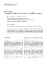
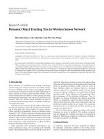
Figure 1: Parallel fusion model with K sensors and one FC. A cen-
sored DSTBC is used for transmission from the sensors to the FC.
ML and GLRT noncoherent FC decision rules and ana-
lyze the performance of the GLRT decision rule. A gradient
algorithm for optimization of the local decision/censoring
threshold is provided in Section 4. Simulation and numer-
ical results are given in Section 5, while some conclusions are
drawninSection6.
Notation. In this paper, bold upper case and lower case
letters denote matrices and vectors, respectively. [
·]
T
,[·]
H
,
ε
{·}, ||·||

2
, |·|,and∪ denote transposition, Hermitian
transposition, statistical expectation, the L
2
-norm of a vec-
tor, the cardinality of a set, and the union of two sets, respec-
tively. In addition, Q(x)  1/
√
2π

∞
x
e
−t
2
/2
dt, I
X
, 0
X×Y
,and
j 
√
−1 denote the Gaussian Q-function, the X ×X identity
matrix, the X
× Y all zeros matrix, and the imaginary unit,
respectively.
2. SYSTEM MODEL
The binary hypothesis testing problem under consideration
is illustrated in Figure 1,whereasetK 

{1, 2, , K} of K
distributed sensors tries to determine the true state of nature
H as being H
0
(the null hypothesis) or H
1
(target-present hy-
pothesis). Typical applications for binary hypothesis testing
include seismic detection, forest fire detection, and environ-
mental monitoring. The a priori probabilities of the two hy-
potheses H
0
and H
1
are denoted as P(H
0
)andP(H
1
), respec-
tively. We assume that P(H
0
) = P(H
1
) = 0.5 throughout this
paper. The details of the system model will be discussed in
the following subsections.
2.1. Local sensor decisions
We assume that the sensor observations are described by
H
0

:x
k
=−1+n
k
, k ∈ K,
H
1
:x
k
= 1+n
k
, k ∈ K,
(1)
S. Yiu and R. Schober 3
where the local observation noise samples n
k
, k ∈ K,are
independent and identically distributed (i.i.d.). For conve-
nience and similar to [8, 9, 11], we assume identical sen-
sors in this paper and model n
k
as real-valued additive white
Gaussian noise (AWGN) with zero mean and variance σ
2

ε
{n
2
k
}, k ∈ K. We note, however, that the generalization of

our results to nonidentical sensors (e.g., sensors with differ-
ent noise variances) is also possible.
Upon receiving its own observation, each sensor makes a
ternary local decision:
u
k
=
⎧
⎪
⎪
⎨
⎪
⎪
⎩
−
1ifx
k
< −d,
1ifx
k
>d,
0 otherwise,
k
∈ K,(2)
where d is the nonnegative decision/censoring threshold.
While u
k
=−1andu
k
= 1 correspond to hypotheses H

0
and H
1
,respectively,u
k
= 0 corresponds to a decision that
is deemed unreliable by the sensor and thus censored. For
future reference, we denote the sets of sensors with u
k
= 0,
u
k
=−1, and u
k
= 1byS, H
0
,andH
1
,respectively.Note
that K
= S ∪H
0
∪ H
1
.
It is not difficult to show that the probabilities of correct
and wrong sensor decision are given by
P
c
= Q


d −1
σ

,
P
w
= Q

d +1
σ

,
(3)
respectively. The probability that a decision is censored is
given by
P
s
= 1 −P
c
− P
w
= 1 −Q

d −1
σ

−
Q


d +1
σ

. (4)
2.2. Noncoherent distributed space-time coding
The general concept of DSTBC was originally proposed in
[13] to achieve a diversity gain in cooperative networks with
decode-and-forward relaying. The DSTBC scheme in [14]is
particularly attractive for application in networks with a large
number of nodes since its decoding complexity is indepen-
dent of the total number of nodes. This scheme consists of
acodeC and a set of signature vectors G. The active relay
nodes
1
encode the (correctly decoded) source information
using a T
× N code matrix Φ ∈ C.Eachactiverelaytrans-
mits a linear combination of the columns of the information-
carrying matrix Φ. The linear combination coefficients for
each node are unique and are collected in a signature vector
g
k
∈ G, g
k

2
2
= 1, k ∈ K,oflengthN.
In this work, we consider the application of the DSTBC
scheme in [14] in WSNs. In particular, sensors encode their

local decisions using a noncoherent DSTBC. Since we con-
sider here a binary hypothesis testing problem, C
={Φ
0
, Φ
1
}
1
The relays which fail to decode the source packet correctly remain silent.
has only two elements. To optimize performance under non-
coherent detection, we choose Φ
0
and Φ
1
to be orthogo-
nal, that is, Φ
H
0
Φ
1
= 0
N×N
and Φ
H
ν
Φ
ν
= I
N
, ν ∈{0, 1}

(cf. [17]). Each sensor is assigned a unique signature vector
g
k
∈ G, g
k

2
2
= 1, k ∈ K,oflengthN. For the design of
deterministic and random signature vector sets G,wereferto
[14, 15] , respectively. The transmitted signal of sensor k is
given by
s
k
=
⎧
⎪
⎪
⎨
⎪
⎪
⎩
√
EΦ
0
g
k
if k ∈ H
0
,

√
EΦ
1
g
k
if k ∈ H
1
,
0
T×1
if k ∈ S,
(5)
where E denotes the transmitted energy of sensor k per code-
word. We note that sensor k transmits the T elements of s
k
in
T consecutive symbol intervals. The total average transmit-
ted energy per information bit is given by E
b
= EK(P
w
+ P
c
).
2.3. Channel model
We assume that the sensors transmit time synchronously and
that the sensor-FC channels are frequency-nonselective and
time-invariant for at least T symbol intervals.
2
Therefore, us-

ing the equivalent complex baseband representation of band-
pass signals, the signal samples received at the FC in T con-
secutive symbol intervals can be expressed as
r
=

k∈H
0
∪H
1
s
k
h
k
+ n =
√
EΦ
0
G
H
0
h
H
0
+
√
EΦ
1
G
H

1
h
H
1
+ n,
(6)
where h
k
and n denote the fading gain of sensor k and a com-
plex AWGN vector, respectively. The columns of the N
×|H
0
|
matrix G
H
0
and N ×|H
1
| matrix G
H
1
contain the signa-
ture vectors of the sensors in H
0
and H
1
,respectively.The
corresponding fading gains are collected in column vectors
h
H

0
and h
H
1
which have lengths |H
0
| and |H
1
|,respectively.
We model the channel gains h
k
, k ∈ K, as i.i.d. zero-mean
complex Gaussian random variables (Rayleigh fading) with
variance σ
2
h
= ε{|h
k
|
2
}=1.
3
The elements of the noise vec-
tor n have variance σ
2
n
= N
0
,whereN
0

denotes the power
spectral density of the underlying continuous-time passband
noise process.
Equation (6) clearly shows the importance of censoring
when applying DSTBCs in WSNs, since incorrect sensor de-
cisions lead to interference. For example, for H
= H
0
,ide-
ally the term involving Φ
1
in (6) would be absent. How-
ever, incorrect decisions may cause some sensors to trans-
mit
√
EΦ
1
g
k
instead of
√
EΦ
0
g
k
. The considered censoring
2
Time synchronous transmission can be accomplished if the relative delays
between the relay nodes are much smaller than the symbol duration. This
is usually a reasonable assumption for low-rate WSN applications. We re-

fer the interested reader to [18] for a more detailed discussion on time
synchronism in the context of WSNs.
3
This model is justified if the distance between any pair of sensors is much
smaller than the distances between the sensors and the FC. The effect of
unequal channel variances is considered in Section 5 (cf. Figure 7).
4 EURASIP Journal on Advances in Signal Processing
scheme reduces the number of incorrect decisions (by choos-
ing d>0) at the expense of reducing the number of sensors
that make a correct decision. However, this disadvantage is
outweighed by the reduction of interference as long as d is
not too large (cf. Section 5). We note that censoring was not
considered in any of the related publications, for example,
[11, 13–15]. For example, in [13–15], DSTBCs were mainly
applied for relay purposes, where a CRC code can be used to
avoid the retransmission of incorrect decisions.
2.4. Processing at fusion center (FC)
The FC makes a decision based on the received vector r and
outputs u
0
= 1 if it decides in favor of H
1
,andu
0
=−1 other-
wise. Different decision rules may be applied at the FC differ-
ing in performance and complexity. In this context, we note
that coherent detection is not feasible in large-scale WSNs
since the FC would have to estimate and track the channel
gains of all sensors. While (6) suggests that only the effective

channels
√
EG
H
0
h
H
0
and
√
EG
H
1
h
H
1
have to be estimated if
distributed space-time coding is applied, this is also not feasi-
ble since the sets H
0
and H
1
typically change after T symbol
intervals (i.e., for every new sensor decision). Therefore, only
noncoherent decision rules will be considered in the next sec-
tion.
3. FC DECISION RULES AND PERFORMANCE
ANALYSIS
In this section, we present the optimum ML and the
generalized-likelihood ratio test (GLRT) noncoherent deci-

sion rules. In addition, we provide a performance analysis
for the GLRT decision rule.
3.1. Optimum maximum-likelihood (ML) decision rule
We first provide the optimum ML decision rule. For this pur-
pose, we introduce the likelihood ratio (LR):
Λ
o
(r) 
f

r |H
1

f

r |H
0

=

H
0
,H
1
f

r |H
0
, H
1


P

H
0
, H
1
|H
1


H
0
,H
1
f

r |H
0
, H
1

P

H
0
, H
1
|H
0


,
(7)
where P(H
0
, H
1
|H
0
) = P
|H
0
|
c
P
|S|
s
P
|H
1
|
w
and P(H
0
, H
1
|H
1
)
= P

|H
1
|
c
P
|S|
s
P
|H
0
|
w
denote the probabilities that the sets H
0
, H
1
occur for H
0
and H
1
, respectively. Since r conditioned on
H
0
, H
1
is a Gaussian vector, the conditional probability den-
sity function (pdf) f (r
|H
0
, H

1
)isgivenby
f

r |H
0
, H
1

=
exp

−
r
H
Br

π
T
det(B)
,(8)
where the T
× T correlation matrix B is defined as B 
ε
{rr
H
|H
0
, H
1

}=E(Φ
0
G
H
0
G
H
H
0
Φ
H
0
+Φ
1
G
H
1
G
H
H
1
Φ
H
1
)+σ
2
n
I
T
.

Now we can express the ML decision rule at the FC as
u
0
=

1ifΛ
o
(r) ≥ 1,
−1ifΛ
o
(r) < 1.
(9)
We note that the sums in the numerator and denominator
of (7)bothhave3
K
terms, that is, the complexity of the ML
decision rule is of orde O(3
K
)andgrowsexponentiallywith
K. In addition, (8) reveals that for the ML decision rule the
FC requires knowledge of the signature vectors of all sensors.
These two assumptions make the implementation of the ML
decision rule difficult, if not impossible in practice. There-
fore, we will provide a low-complexity suboptimum FC de-
cision rule in the next subsection.
3.2. GLRT decision rule
The received vector can be expressed as
r
= Φh
eff

+ n
eff
, Φ ∈

Φ
0
, Φ
1

. (10)
If H
0
is the true hypothesis Φ = Φ
0
, h
eff

√
EG
H
0
h
H
0
,and
n
eff

√
EΦ

1
G
H
1
h
H
1
+ n, while if H
1
is true Φ = Φ
1
, h
eff

√
EG
H
1
h
H
1
,andn
eff

√
EΦ
0
G
H
0

h
H
0
+ n.
Equation (10) suggests a two-step GLRT approach for the
estimation of the transmitted codewor Φ. In the first step, h
eff
is estimated assuming Φ is known, and in the second step the
channel estimate

h
eff
is used to detect Φ. Since the correlation
matrix of the effective noise n
eff
depends on G
H
1
or G
H
0
, the
ML estimate for h
eff
and thus the resulting GLRT decision
rule depend on the signature vectors. Therefore, the com-
plexity of this GLRT decision rule is still exponential in K.
To avoid this problem we resort to the simpler least-squares
(LS) approach to channel estimation. The LS channel esti-
mate is given by


h
eff
 arg min
h
eff

r − Φh
eff

2
2

= Φ
H
r. (11)
Now, the GLRT decision rule can be expressed as

Φ
= arg min
Φ∈{Φ
0
,Φ
1
}


r − Φ

h

eff

2
2

=
arg max
Φ∈{Φ
0
,Φ
1
}

Φ
H
r
2
2

,
(12)
where all irrelevant terms have been dropped. The FC output
u
0
=−1if

Φ = Φ
0
,andu
0

= 1if

Φ = Φ
1
. Clearly, the GLRT
decision rule does not require CSI and the FC does not have
to know the signature vectors of the sensors.
3.3. Performance analysis for GLRT decision rule
For the optimum ML decision rule, a closed-form perfor-
mance analysis does not seem to be feasible. However, for-
tunately such an analysis is possible for the more practical
GLRT decision rule. In particular, the BER can be expressed
as
P
e
= P

u
0
= 1 |H
0

P

H
0

+ P

u

0
=−1|H
1

P

H
1

.
(13)
Since the considered signaling scheme is symmetric in H
0
and H
1
,(13) can be simplified to P
e
= P(u
0
= 1|H
0
). Ex-
panding now P(u
0
= 1|H
0
)leadsto
P
e
=


H
0
,H
1
P

u
0
= 1 |H
0
, H
1

P

H
0
, H
1
|H
0

, (14)
S. Yiu and R. Schober 5
where P(u
0
= 1 |H
0
, H

1
) denotes the probability that u
0
= 1
is detected assuming that u
k
=−1fork ∈ H
0
and u
k
=
1fork ∈ H
1
,andP(H
0
, H
1
|H
0
) is given in Section 3.1.
Exploiting the orthogonality of Φ
0
and Φ
1
and using (6)and
(12), P(u
0
= 1 |H
0
, H

1
) can be expressed as
P

u
0
= 1 |H
0
, H
1

=
P

Δ < 0|H
0
, H
1

, (15)
where
Δ 
x
2
2
−y
2
2
,
x 

√
EG
H
0
h
H
0
+ Φ
H
0
n,
y 
√
EG
H
1
h
H
1
+ Φ
H
1
n.
(16)
Since Δ is a quadratic form of Gaussian random variables,
the Laplace transform Φ
Δ
(s)ofthepdfofΔ can be obtained
as
Φ

Δ
(s) =
1

N
i
=1

1+sλ
x
i


N
i
=1

1 − sλ
y
i

, (17)
where λ
x
i
and λ
y
i
denote the eigenvalues of the N ×N matri-
ces

D
x
 ε{xx
H
}=EG
H
0
G
H
H
0
+ σ
2
n
I
N
,
D
y
 ε{yy
H
}=EG
H
1
G
H
H
1
+ σ
2

n
I
N
,
(18)
respectively. Thus, P(u
0
= 1 |H
0
, H
1
) can be calculated from
[19]
P

u
0
= 1 |H
0
, H
1

=
1
2πj
c+ j∞

c−j∞
Φ
Δ

(s)
s
ds, (19)
where c is a small positive constant in the region of conver-
gence of the integral. The integral in(19) can be either com-
puted numerically using Gauss-Chebyshev quadrature rules
[19] or exactly using [20, 21]
P

u
0
= 1 |H
0
, H
1

=−

RHS poles
Residue

Φ
Δ
(s)
s

, (20)
where RHS stands for the right-hand side of the complex
plane. The BER at the FC for the GLRT decision rule can be
readily obtained by combining (14)and(19).

4. OPTIMIZATION OF CENSORING THRESHOLD d
Since a closed-form calculation of the optimum decision/
censoring threshold d which minimizes P
e
doesnotseemto
be possible, we derive here a gradient algorithm for recursive
optimization of d. This algorithm is given by [22]
d[i +1]
= d[i]+δ
∂P
e
∂d[i]
, (21)
where i is the discrete iteration index and δ is the adaptation
step size. Using (14) the gradient in (21) can be expressed as
∂P
e
∂d
=

H
0
,H
1
P

u
0
= 1 |H
0

, H
1

∂P

H
0
, H
1
|H
0

∂d
, (22)
where we have used the fact that P(u
0
= 1 |H
0
, H
1
) is in-
dependent of d and the remaining partial derivative is given
by
∂P

H
0
, H
1
||H

0

∂d
=|S|P
|S|−1
s
P
|H
0
|
c
P
|H
1
|
w
∂P
s
∂d
+
|H
0
|P
|S|
s
P
|H
0
|−1
c

P
|H
1
|
w
∂P
c
∂d
+
|H
1
|P
|S|
s
P
|H
0
|
c
P
|H
1
|−1
w
∂P
w
∂d
.
(23)
Using (3), (4) and the fundamental theorem of calculus [23],

the derivatives in (23) can be expressed as
∂P
w
∂d
=−
1
√
2πσ
e
−(d+1)
2
/2σ
2
,
∂P
c
∂d
=−
1
√
2πσ
e
−(d−1)
2
/2σ
2
,
∂P
s
∂d

=
1
√
2πσ

e
−(d+1)
2
/2σ
2
+ e
−(d−1)
2
/2σ
2

.
(24)
For d
= 0, we have |S|=0 and since ∂P
w
/∂d < 0and
∂P
c
/∂d < 0weobtain∂P
e
/∂d < 0. On the other hand, for
d
→∞,weget|H
0

|→0and|H
1
|→0 which results in ∂P
e
/∂d >
0.
4
Therefore, by the mean value theorem, ∂P
e
/∂d = 0isvalid
for at least one value of 0
≤ d<∞ corresponding to at least
one local minimum of P
e
[23]. Although numerical evidence
shows that there is exactly one local minimum (which there-
fore is also the global minimum), we cannot formally prove
this due to the complexity of the involved expressions. Nev-
ertheless, the above considerations suggest that we initialize
the gradient algorithm with d[0]
= 0 corresponding to the
case of no censoring. The solution found by the algorithm is
then guaranteed to yield a performance not worse than that
of the no censoring case. Numerical examples will be given
in the next section.
We note that d will typically be calculated at the FC and
the value of d has to be conveyed to the sensors over a feed-
back channel. However, this feedback channel can be very
low rate assuming that the statistical properties of the for-
ward channel and the sensors vary only slowly with time.

5. SIMULATION RESULTS
In this section, we provide some numerical and simulation
results for the proposed censored DSTBCs and the system
model introduced in Section 2. We assume that T
= 8sym-
bol intervals are available for transmission of one informa-
tion bit, that is, orthogonal matrices Φ
0
and Φ
1
can be found
for N
≤ 4. Here, we consider N = 1, N = 2, and N = 4, and
generate Φ
0
and Φ
1
from the 8 × 8 Hadamard matrix H
8
,
where the orthogonal columns of H
8
are normalized to unit
length. For example, for N
= 2Φ
0
consists of the first two
columns of H
8
,whereasΦ

1
consists of the third and fourth
4
In fact, it can be shown that ∂P
e
/∂d approaches zero from above if d→∞
corresponding to the maximum BER of P
e
= 0.5.
6 EURASIP Journal on Advances in Signal Processing
0246810
×10
2
i
0
0.2
0.4
0.6
0.8
1
1.2
1.4
d
N
= 1, δ = 3
N
= 2, δ = 1
N
= 4, δ = 1
(a)

0246810
×10
2
i
10
−3
10
−2
10
−1
P
e
N = 1, δ = 3
N
= 2, δ = 1
N
= 4, δ = 1
(b)
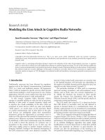
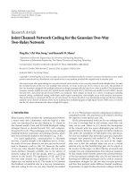
Figure 2: d and P
e
versus iteration number i for a WSN with K = 30
sensors using DSTBCs with N
= 1, 2, and 4. 10 log
10
(E
b
/N
0
) =
15 dB, σ

2
= 1/4.
column of H
8
. For the set of signature vectors G,weadopted
the gradient sets described in [14]. Unless stated otherwise,
the sensors have a local noise variance of σ
2
= 1/4corre-
sponding to a signal-to-noise ratio (SNR) of 6 dB and we
assume the suboptimum GLRT decision rule and P
e
at the
FC are obtained using the analytical results presented in Sec-
tion 3.3.
5
d and P
e
versus i. First, we investigate the behavior of the
adaptive algorithm described in Section 4 for optimization of
d. Figure 2 shows d and the corresponding BER P
e
at the FC
as a function of the iteration number i for N
= 1, 2, and 4, re-
spectively. The considered WSN had K
= 30 sensors and the
channel SNR was 10 log
10
(E

b
/N
0
) = 15 dB. d[i] was initial-
ized with 0 and the step size parameter was chosen to achieve
a fast convergence while avoiding instabilities. As can be ob-
served from Figure 2 the adaptive algorithm significantly im-
proves the BER over the iterations. While d itself requires
more than 600 iterations to converge to the final optimum
value, P
e
does practically not change after more than 180 it-
erations for all considered cases. It is interesting to note that
the optimum value for d decreases with increasing N, that is,
for larger N less censoring should be applied. The reason for
this behavior is that the maximum achievable diversity order
of a DSTBC is N (cf. [14]) and therefore, the performance
of the DSTBC improves notably with increasing number of
transmitting sensors only until N sensors transmit. If more
than N sensors transmit, the diversity order does not further
improve and only a small additional coding gain can be real-
5
We note that we confirmed the analytical BER results for the GLRT de-
cision rule presented in Section 3.3 by simulations. However, we do not
show the simulation results here for conciseness.
6 8 10 12 14 16 18 20
10 log
10
(E
b

/N
0
)(dB)
10
−4
10
−3
10
−2
10
−1
P
e
σ
2
= 1/4,d = 0
σ
2
= 1/4,d = d
opt
σ
2
= 0, d = 0
N
= 1
N
= 2
N
= 4
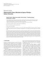
Figure 3: P

e
versus 10log
10
(E
b
/N
0
)foraWSNwithK = 30 sensors
using DSTBCs with N
= 1, 2, and 4. Considered cases: error-free
local sensor decisions (σ
2
= 0, d = 0), noisy sensor decisions with-
out censoring (σ
2
= 1/4, d = 0), and noisy sensor decisions with
optimum censoring (σ
2
= 1/4, d = d
opt
).
ized. On the other hand, less censoring means that more er-
roneous decisions are forwarded to the FC which may negate
the additional coding gain.
P
e
versus 10 log
10
(E
b

/N
0
). In Figure 3, we consider the
BER achievable with the proposed censored DSTBCs at the
FC of a WSN with K
= 30 sensors as a function of the
channel SNR 10 log
10
(E
b
/N
0
). For each considered N,we
compare the BER for error-free local sensor decisions (σ
2
=
0, d = 0), noisy sensor decisions without censoring (σ
2
=
1/4, d = 0), and noisy sensor decisions with censoring
(σ
2
= 1/4, d = d
opt
), where d
opt
denotes the optimum deci-
sion/censoring threshold found with the gradient algorithm.
Figure 3 clearly shows that DSTBCs suffer from a significant
performance degradation due to erroneous decisions if cen-

soring is not applied. Fortunately, with censoring this perfor-
mance degradation can be avoided and a performance close
to that of error-free local decisions can be achieved. Figure 3
also nicely illustrates the diversity gain that can be realized
with censored DSTBCs.
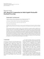
P
e
versus K. In Figure 4, we investigate the dependence of
the BER on the total number of sensors in the network for
10 log
10
(E
b
/N
0
) = 15 dB. In particular, we show in Figure 4
the BER for error-free local sensor decisions and the GLRT
decision rule at the FC (σ
2
= 0, d = 0), noisy sensor deci-
sions with censoring and the GLRT decision rule at the FC
(σ
2
= 1/4, d = d
opt
), and noisy sensor decisions with censor-
ing and the ML decision rule at the FC (σ
2
= 1/4, d = d
opt

).
6
6
We note that we use for the ML decision rule also the decision/censoring
threshold d
opt
found by the proposed gradient algorithm which is based
on the GLRT decision rule. Therefore, this threshold is not strictly opti-
mum for the ML decision rule.
S. Yiu and R. Schober 7
51015202530
K
10
−2
P
e
σ
2
= 1/4,d = d
opt
,GLRT
σ
2
= 1/4,d = d
opt
,ML
σ
2
= 0, d = 0
N

= 1
N
= 2
N
= 4
Figure 4: P
e
versus total number of sensors K for aWSN using DST-
BCs with N
= 1, 2, and 4. 10 log
10
(E
b
/N
0
) = 15 dB. Numerical re-
sults for error-free local sensor decisions and GLRT decision rule
(σ
2
= 0, d = 0), numerical results for noisy sensor decisions with
censoring and GLRT decision rule (σ
2
= 1/4, d = d
opt
), and sim-
ulation results for noisy sensor decisions with censoring and ML
decision rule (σ
2
= 1/4, d = d
opt

).
The results for the GLRT decision rule were obtained numer-
ically based on the analytical results in Section 3.3,whereas
Monte Carlo simulation was used to obtain the results for
the ML decision rule. For complexity reasons, for the latter
case, we only show the results for K
≤ 5. For error-free local
sensor decisions, BER is constant for K>Nsince the diver-
sity order is limited to N and the DSTBC achieves the same
performance as the related STBC C for colocated antennas if
all K>Nsensors transmit. The censored DSTBC with noisy
sensor decisions approaches the performance of the DSTBC
with error-free sensor decisions as the number of sensors in-
creases. This is due to the fact that as K increases the deci-
sion/censoring threshold d
opt
increases making the transmis-
sion of erroneous sensor decisions less likely. Figure 4 also
shows that the GLRT decision rule is almost optimum and
only small additional gains are possible if the significantly
more complex ML decision rule is used.
P
e
and d versus N. Assuming the GLRT decision rule and
10 log
10
(E
b
/N
0

) = 15 dB at the FC, Figure 5 shows P
e
and
the corresponding optimum decision threshold d as a func-
tion of N for K
= 1, 2, 4, 10 and 30. Similar to the obser-
vation we made in Figure 2, d decreases for increasing sig-
nature vector length N for all K.Aswehavementionedbe-
fore, the maximum achievable diversity order for DSTBC is
N.ForagivenK, a smaller d allows more sensors to be active
and thus exploits the the extra diversity benefit provided by
the longer signature vectors. This figure also shows that d in-
creases for increasing K. This can be also explained easily. For
agivend and N, increasing K allows more sensors to trans-
mit. However, our scheme only requires a certain number of
sensors to be active to exploit the full diversity benefit and
1234
N
0
0.01
0.02
0.03
0.04
0.05
0.06
0.07
P
e
K = 1
K

= 2
K
= 4
K
= 10
K
= 30
(a)
1234
N
0
0.2
0.4
0.6
0.8
1
1.2
1.4
d
K
= 1
K
= 2
K
= 4
K
= 10
K
= 30
(b)

Figure 5: P
e
and d versus N for aWSN with K sensors. σ
2
= 1/4
and 10 log
10
(E
b
/N
0
) = 15 dB. GLRT fusion rule is shown for all K
(solid curves) and ML fusion rule is shown for K
= 1 and 2 (dashed
curve).
achieve a certain target BER. On the other hand, increasing
d decreases the chance of having erroneous decisions being
transmitted to the FC. This suggests that our scheme tries to
maximize the performance by only allowing the minimum
number of sensors (with quality decisions) to transmit. Fi-
nally, it is interesting to see that the P
e
performance actually
deteriorates for N>Kfor the GLRT fusion rule. This is be-
cause for N>Kthe GLRT fusion rule implicitly estimates
the N
×1effective channel vector

h
eff

in a noisy environment
(cf. (11)) whereas the underlying channel vectors, h
H
0
and
h
H
1
, have a smaller dimensionality K. The increased dimen-
sionality causes a larger channel estimation error while no
diversity benefit is achieved because the maximum diversity
order is limited to K [14]. In light of this degradation for the
GLRT fusion rule, we also simulated the ML fusion rule for
K
= 1andK = 2 (dashed curves) and clearly, as expected,
the ML decision rule does not suffer from the same degra-
dation. We note that in the practically more relevant case of
N<KML and GLRT decision rules have similar perfor-
mances (cf. Figure 4).
P
e
and d versus SNR of local sensors. We investigate the ef-
fect of local sensor observation noise on the P
e
performance
in Figure 6.Inparticular,weplotP
e
versustheSNRoflocal
sensors 10log
10

(1/σ
2
)fordifferent K and N. We assume the
GLRT fusion rule at the FC and the corresponding optimum
decision threshold d is also depicted. Furthermore, the chan-
nel SNR is fixed to 10 log
10
(E
b
/N
0
) = 15 dB for all cases. As
expected, the network with K
= 30 sensors performs better
than the network with K
= 10 sensors for any N regardless
of the sensor observation noise. However, this gain is mini-
mal for large sensor SNR. This is because as the sensor SNR
8 EURASIP Journal on Advances in Signal Processing
−50 51015
10 log
10
(1/σ
2
)(dB)
0
0.02
0.04
0.06
0.08

0.1
0.12
0.14
0.16
P
e
N = 1
N
= 2
N
= 4
K
= 10
K
= 30
(a)
−50 5 1015
10 log
10
(1/σ
2
)(dB)
0
0.5
1
1.5
2
2.5
3
3.5

d
N
= 1
N
= 2
N
= 4
K
= 30
K
= 10
(b)
Figure 6: P
e
and d versus 10 log
10
(1/σ
2
)foraWSNwithK = 10,
and 30 sensors and DSTBC with N
= 1,2, and 4. 10log
10
(E
b
/N
0
) =
15 dB.
6 8 10 12 14 16 18 20
10 log

10
(E
b
/N
0
)(dB)
10
−4
10
−3
10
−2
10
−1
P
e
r/d = 0.6
r/d
= 0.4
r/d
= 0.2
r/d
= 0
N
= 1
N
= 2
N
= 4
Figure 7: P

e
versus 10log
10
(E
b
/N
0
)foraWSNwithK = 30 sensors
using DSTBCs with N
= 1, 2, and 4. σ
2
= 1/4 and i.n.d. Rayleigh
fading channels.
increases, most of the sensor decisions will be correct and
less censoring is required. This phenomenon is clearly sup-
ported by the corresponding d versus 10 log
10
(1/σ
2
) figure
where the optimum decision threshold d approaches zero for
increasing sensor SNR. In addition, as more sensors transmit,
the maximum achievable diversity order N and the channel
SNR will be the ultimate factors which determine P
e
and
therefore, for a given N, the BER curves for K
= 10 and
K
= 30 converge to the same value for large local sensor SNR.

I.n.d. Rayleigh fading. Until now, we have been consider-
ing i.i.d. Rayleigh fading channels. In our last example, we
consider independent and nonidentically distributed (i.n.d.)
fading channels. In particular, we consider a network with
K
= 30 sensors and the sensor nodes are uniformity dis-
tributed in a circle with radius r and the distance from the
center of the circle to the FC is d. We assume i.n.d. Rayleigh
fading between the sensors and the FC and the received
power decreases as d
−α
k
,whered
k
is the distance measured
from sensor k to the FC and α
= 3 is the path loss exponent.
Figure 7 depicts the simulated P
e
versus 10 log
10
(E
b
/N
0
)for
different r/d ratios. For a given N, the decision threshold d
was optimized for r/d
= 0 (corresponding to i.i.d. fading)
and it was then used also for r/d > 0. It can be seen from the

figure that, as expected, P
e
increases with increasing r/d.It
is also interesting to note that the performance degradation
is larger for larger N. This can be explained as follows. For a
given network size K,aswehaveseeninFigures4 and 5, d
decreases for increasing N. Since a smaller censoring thresh-
old d corresponds to a larger number of active sensors, more
sensors are negatively affected by the i.n.d. channels resulting
in the greater performance degradation for larger N.
6. CONCLUSION
In this paper, we have considered the application of nonco-
herent DSTBCs in WSNs. We have introduced censoring as
an efficient method to overcome the negative effects of erro-
neous local sensor decisions on the performance of the non-
coherent DSTBC. Furthermore, we have derived optimum
ML and suboptimum GLRT FC decision rules, and we have
analyzed the performance of the latter decision rule. Based
on this analysis, we have devised a gradient algorithm for
recursive optimization of the decision/censoring threshold.
Numerical and simulation results have shown the effective-
ness of censoring which eliminates the effect of local deci-
sion errors for practically relevant BERs if the number of sen-
sors in the network K is greater than the length of the signa-
ture vectors N or in other words, if there are enough sensors
to exploit the diversity benefit provided by the DSTBC. Fi-
nally, our results have shown that the suboptimum GLRT fu-
sion rule performs very close to the optimum ML fusion rule
while having a very low complexity and allowing noncoher-
ent detection at the FC.

ACKNOWLEDGMENTS
This paper was presented in part at the IEEE Wireless Com-
munications & Networking Conference, Hong Kong, China,
March 2007.
REFERENCES
[1] R. R. Tenney and N. R. Sandell Jr., “Detection with distributed
sensors,” IEEE Transactions on Aerospace and Electronic Sys-
tems, vol. 17, no. 4, pp. 501–510, 1981.
[2] J. N. Tsitsiklis, “Decentralized detection,” in Advances in Statis-
tical Signal Processsing, vol. 2, pp. 297–344, JAI Press, Green-
wich, Conn, USA, 1993.
S. Yiu and R. Schober 9
[3] R. Viswanathan and P. K. Varshney, “Distributed detection
with multiple sensors—part I: fundamentals,” Proceedings of
the IEEE, vol. 85, no. 1, pp. 54–63, 1997.
[4] R. S. Blum, S. A. Kassam, and H. V. Poor, “Distributed detec-
tion with multiple sensors—part II: advanced topics,” Proceed-
ings of the IEEE, vol. 85, no. 1, pp. 64–79, 1997.
[5] P. K. Varshney, Distributed Detection with Multiple Sensors,
Springer, Berlin, Germany, 1997.
[6] J J. Xiao and Z Q. Luo, “Universal decentralized detection in
a bandwidth-constrained sensor network,” IEEE Transactions
on Signal Processing, vol. 53, no. 8, pp. 2617–2624, 2005.
[7] B. Chen, R. Jiang, T. Kasetkasem, and P. K. Varshney, “Chan-
nel aware decision fusion in wireless sensor networks,” IEEE
Transactions on Signal Processing, vol. 52, no. 12, pp. 3454–
3458, 2004.
[8] R. Niu, B. Chen, and P. K. Varshney, “Fusion of decisions
transmitted over Rayleigh fading channels in wireless sen-
sor networks,” IEEE Transactions on Signal Processing, vol. 54,

no. 3, pp. 1018–1027, 2006.
[9] R. Jiang and B. Chen, “Fusion of censored decisions in wireless
sensor networks,” IEEE Transactions on Wireless Communica-
tions, vol. 4, no. 6, pp. 2668–2673, 2005.
[10] C. Rago, P. Willett, and Y. Bar-Shalom, “Censoring sensors:
a low-communication-rate scheme for distributed detection,”
IEEE Transactions on Aerospace and Electronic Systems, vol. 32,
no. 2, pp. 554–568, 1996.
[11] T. Ohtsuki, “Performance analysis of statistical STBC cooper-
ative diversity using binary sensors with observation noise,” in
Proceedings of the 62nd IEEE Vehicular Technology Conference
(VTC ’05), vol. 3, pp. 2030–2033, Dallas, Tex, USA, September
2005.
[12] S. M. Alamouti, “A simple transmit diversity technique for
wireless communications,” IEEE Journal on Selected Areas in
Communications, vol. 16, no. 8, pp. 1451–1458, 1998.
[13] J. N. Laneman and G. W. Wornell, “Distributed space-time-
coded protocols for exploiting cooperative diversity in wireless
networks,” IEEE Transactions on Information Theory, vol. 49,
no. 10, pp. 2415–2425, 2003.
[14] S. Yiu, R. Schober, and L. Lampe, “Distributed space-time
block coding,” IEEE Transactions on Communications, vol. 54,
no. 7, pp. 1195–1206, 2006.
[15] B. S. Mergen and A. Scaglione, “Randomized space-time
coding for distributed cooperative communication,” in Pro-
ceedings of IEEE International Conference on Communications
(ICC ’06), vol. 10, pp. 4501–4506, Istanbul, Turkey, June 2006.
[16] J. N. Laneman, D. N. C. Tse, and G. W. Wornell, “Cooperative
diversity in wireless networks: efficient protocols and outage
behavior,” IEEE Transactions on Information Theory, vol. 50,

no. 12, pp. 3062–3080, 2004.
[17] B. M. Hochwald and T. L. Marzetta, “Unitary space-time mod-
ulation for multiple-antenna communications in Rayleigh flat
fading,” IEEE Transactions on Information Theory, vol. 46,
no. 2, pp. 543–564, 2000.
[18] X. Li, M. Chen, and W. Liu, “Application of STBC-encoded
cooperative transmissions in wireless sensor networks,” IEEE
Signal Processing Letters, vol. 12, no. 2, pp. 134–137, 2005.
[19] E. Biglieri, G. Caire, G. Taricco, and J. Ventura-Traveset,
“Computing error probabilities over fading channels: a uni-
fied approach,” European Transactions on Telecommunications,
vol. 9, no. 1, pp. 15–25, 1998.
[20] J. K. Cavers and P. Ho, “Analysis of the error performance of
trellis-coded modulations in Rayleigh-fading channels,” IEEE
Transactions on Communications, vol. 40, no. 1, pp. 74–83,
1992.
[21] E. B. Saff and A. D. Snider, Fundamentals of Complex Analysis
for Mathematics, Science and Enginee ring, Prentice Hall, Upper
Saddle River, NJ, USA, 2nd edition, 1993.
[22] J. Nocedal and S. J. Wright, Numerical Optimization, Springer,
New York, NY, USA, 1999.
[23] R. A. Adams, Single Variable Calculus, Addison-Wesley, Read-
ing, Mass, USA, 1995.