Báo cáo hóa học: " Research Article Robust Abandoned Object Detection Using Dual Foregrounds" pptx

Hindawi Publishing Corporation
EURASIP Journal on Advances in Signal Processing
Volume 2008, Article ID 197875, 11 pages
doi:10.1155/2008/197875
Research Article
Robust Abandoned Object Detection Using Dual Foregrounds
Fatih Porikli,
1
Yuri Ivanov,
1
and Tetsuji Haga
2
1
Mitsubishi Electric Research Labs (MERL), 201 Broadway, Cambridge, MA 02139, USA
2
Mitsubishi Electric Corp. Advanced Technology R&D Center, Amagasaki, 661-8661 Hyogo, Japan
Correspondence should be addressed to Fatih Porikli,
Received 25 January 2007; Accepted 28 August 2007
Recommended by Enis Ahmet C¸etin
As an alternative to the tracking-based approaches that heavily depend on accurate detection of moving objects, which often fail
for crowded scenarios, we present a pixelwise method that employs dual foregrounds to extract temporally static image regions.
Depending on the application, these regions indicate objects that do not constitute the original background but were brought into
the scene at a subsequent time, such as abandoned and removed items, illegally parked vehicles. We construct separate long- and
short-term backgrounds that are implemented as pixelwise multivariate Gaussian models. Background parameters are adapted
online using a Bayesian update mechanism imposed at different learning rates. By comparing each frame with these models, we
estimate two foregrounds. We infer an evidence score at each pixel by applying a set of hypotheses on the foreground responses, and
then aggregate the evidence in time to provide temporal consistency. Unlike optical flow-based approaches that smear boundaries,
our method can accurately segment out objects even if they are fully occluded. It does not require on-site training to compensate
for particular imaging conditions. While having a low-computational load, it readily lends itself to parallelization if further speed
improvement is necessary.
Copyright © 2008 Fatih Porikli et al. This is an open access article distributed under the Creative Commons Attribution License,

which permits unrestricted use, distribution, and reproduction in any medium, provided the original work is properly cited.
1. INTRODUCTION
Conventional approaches on abandoned item detection can
be grouped as motion detectors [1–3], object classifiers [4],
and tracking-based analytics approaches [5–10].
In [2], a dense optical flow map is estimated to infer the
foreground objects moving in opposite directions, moving
in a group, and staying stationary by predetermined rules.
In [3], a pixel-based method for characterizing objects intro-
duced into the static scene by comparing the background im-
age estimated from the current frame with the previous ones
is described. This approach requires storing as many back-
grounds as the minimum detection duration in the memory
and causes ghost detections even after the abandoned item is
removed from the scene.
Recently, an online classifier [4] that incorporates a
boosting-based feature selection to label image blocks as
background, valid objects, and unidentified regions is pre-
sented. This method adapts itself to the depicted scene, how-
ever, fails short of discriminating moving objects from sta-
tionary ones. Classifier-based methods face with the chal-
lenge of dealing with unknown object type as such objects
can vary from small luggage to ski bags.
Aconsiderableamountofeffort has been devoted to hy-
pothesize abandoned items by analyzing object trajectories
[5–7, 9, 10] in multicamera setups. In principle, these meth-
ods require solving a harder problem of object initializa-
tion and tracking as an intermediate step in order to iden-
tify the parts of the video frames corresponding to an aban-
doned object. It is often assumed that the background scene

is nearly static or periodically varying, while the foreground
comprises groups of pixels that are different from the back-
ground. However, object detection in crowded scenes, espe-
cially for uncontrolled real-life situations, is problematic due
to the partial occlusions, heavy shadows, people entering the
scene together, and so forth. Moreover, object appearance is
often indiscriminative as people tend to dress in similar col-
ors, which leads inaccurate tracking results.
For static camera setups, background subtraction pro-
vides strong cues for apparent motion statistics. Various
background generation methods have been employed in a
quest for a system that is robust to changing illumination
conditions, appearance variations, shadows, camera jitter,
and severe noise. Parametric mixture models are employed
to handle such variations. Stauffer and Grimson [11]pro-
pose an expectation maximization- (EM-) based adaptation
2 EURASIP Journal on Advances in Signal Processing
Foreground
long
Foreground
short
Hypothesis
Image
I
Change
Moving objectChange
No
change
Candidate
abandoned object

No
change
Change
Uncovered
background
No
change
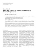
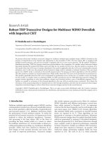
Scene background
Figure 1: Hypotheses on long- and short-term foregrounds.
method to learn a mixture of Gaussians with predetermined
number of models at each pixel using fixed learning parame-
ters. The online EM update causes a weak model, which has a
larger variance, to be dissolved into a dominant model, which
has a smaller variance in case the mean value of the weak
model is close to the mean of the dominant one. To address
this issue, Porikli and Tuzel [12] develop an online Bayesian
update mechanism for adaptation multivariate Gaussian dis-
tributions. This method estimates the number of necessary
layers for each pixel and the posterior distributions of mean
and covariance of each layer by assuming the data to be nor-
mally distributed with mean and covariance as random vari-
ables.
There are other variants of the mixture of models that use
modified feature spaces, image gradients, optical flow, and
region segmentation [13–15]. Instead of iteratively updating
models as mixture methods, nonparametric kernel density
estimation [16] stores a large number of previous frames and
estimates weights of multiple kernel functions. Since both
memory and computational complexity proportionally in-
creases with the number of stored frames, kernel methods

are usually impractical for real-time applications.
There exists a class of problems that cannot be solved by
the traditional foreground-background detection methods.
For instance, objects deliberately abandoned in public places,
such as suitcases, packages, do not fall into either of these
two categories. They are static; therefore, they should be la-
beled as background. On the other hand, they should not be
ignored as they do not belong to the original scene back-
ground. Depending on the learning rate, the pixels corre-
sponding to the temporary static objects can be mistaken as a
part of the scene background (in case of a high-learning rate),
or grouped with the moving regions (low-learning rate). A
single background is not sufficient to separate the temporar-
ily static pixels from the scene background.
In this paper, we propose a pixel-based method that em-
ploys dual foregrounds. Our motivation is that by chang-
ing the background learning rate, we can adjust how soon a
static object should be blended into the background. There-
fore, temporarily static image regions can be distinguished
from the longer term background and moving regions by
analyzing multiple foregrounds of different learning rates.
This simple idea is wrapped into our adaptive background
estimation algorithm, where the slowly adapting background
and the fast adapting foreground are aggregated into an evi-
dence image. We impose different learning rates by process-
ing video at different temporal resolutions. The background
models have identical initial parameters, thus they require
minimal fine tuning in the setup stage. The evidence statistics
are used to extract temporarily static image areas, which may
correspond to abandoned items, illegally parked vehicles, ob-

jects removed from the scene, and so forth, depending on the
application.
Our method does not require object initialization, track-
ing, or offline training. It accurately segments objects even
if they are fully occluded. It has a very low-computational
load and readily lends itself to parallelization if further speed
improvements are necessary. In the subsequent sections, we
give details of the dual foregrounds, show Bayesian adapta-
tion method, and present results on real-world data.
2. DUAL FOREGROUNDS
To detect an abandoned item (or an illegally parked vehicle,
removed article, etc.), we need to know how it alters the tem-
poral and spatial statistics of the video data. We built our
method on the fact that an abandoned item is not a part
of the original scene, it was brought into the scene not that
long ago, and it remained still after it has been left. In other
words, it is a temporarily static object which was not there be-
fore. This means that by learning the prolonged static scene
and the moving foreground regions, we can hypothesize on
whether a pixel corresponds to an abandoned item or not.
A scene background can be determined by maintaining
a statistical model that captures the most consistent modes
of the color distribution of each pixel in extended durations
of time. From this background, the changed pixels that do
not fit into the statistical models are obtained. However, de-
pending on the learning rate, the pixels corresponding to the
temporary static objects can be mistaken as a part of the
scene background (higher-learning rates), or grouped with
the moving regions (lower-learning rates). A single back-
ground is not sufficient to separate the temporarily static pix-

els from the scene background.
As opposed to single background approaches, we use
two backgrounds to obtain both the prolonged (long-term)
background B
L
and the temporarily static (short-term) back-
ground B
S
. Note that it is possible to improve the temporal
granularity by employing more than two backgrounds at dif-
ferent learning rates. Each of these backgrounds is defined
as a mixture of Gaussian models. We represent a pixel as
layers of 3D multivariate Gaussians where each dimension
corresponds to a color channel. Each layer models to a dif-
ferent appearance of the pixel. We perform our operations
on the RGB color space. We apply a Bayesian update mech-
anism. At each update, at most one layer is updated with
the current observation. This assures the minimum over-
lap over the layers. We also determine how many layers are
necessary for each pixel and use only those layers during
the foreground segmentation phase. This is performed with
Fatih Porikli et al. 3
Background confidence
Change
label
Background
Foreground
Decision line
Long-term convergence line
Time

Moving object
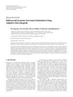
Left-behind item Scene background
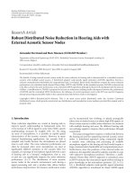
Figure 2: The confidence of the long-term and short-term background models (vertical axis) changes differently for ordinary objects (mov-
ing or temporarily stationary ones), abandoned items, and scene background.
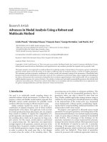
(a) (b) (c) (d)
Alarm!
(e)
Original
(f)
F
L
(g)
F
S
(h)
E
(i)
Alarm!
Result
(j)
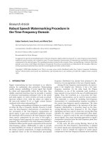
Figure 3: First row: t = 350. Second row: t = 630. The long-term foreground F
L
captures moving objects and temporarily static regions.
The short-term foreground F
S
captures only moving objects. The evidence E gets greater as the object stays longer.
an embedded confidence score. Both of the backgrounds
have identical initial parameters, such as the initial mean
and variance of the marginal posterior distribution, the de-
grees of freedom, and the scale matrix, except the number

of the prior measurements, which is used as a learning para-
meter.
At every frame, we estimate the long and short term
foregrounds by comparing the current frame I by the back-
ground models B
L
and B
S
. We obtain two binary foreground
masks F
L
and F
S
,whereF(x, y) = 1 indicates that the pixel
(x, y) is changed. The long term foreground mask F
L
shows
the color variations in the scene that were not there before
including moving objects, temporarily static objects, as well
as moving cast shadows and illumination changes that the
background models fail to adapt. The short-term foreground
mask F
S
contains the moving objects, noise, and so forth. De-
pending on the foreground mask values, we postulate the fol-
lowing hypotheses as shown in Figure 1.
(1) F
L
(x, y) = 1andF
S

(x, y) = 1, where (x, y) is a pixel
that may correspond to a moving object since I(x, y)
does not fit any backgrounds.
(2) F
L
(x, y) = 1andF
S
(x, y) = 0, where (x, y) is a pixel
that may correspond to a temporarily static object.
(3) F
L
(x, y) = 0andF
S
(x, y) = 1, where (x, y) is a scene
background pixel that was occluded before.
(4) F
L
(x, y) = 0andF
S
(x, y) = 0, where (x, y) is a scene
background pixel since its value I(x, y) fits both back-
grounds B
L
and B
S
.
The short term background is updated at a higher-
learning rate than the long-term background. Thus, the
short-term background adapts to the underlying distribu-
tion faster and the changes in the scene are blended more

rapidly. In contrast, the long-term background is more resis-
tant against the changes.
4 EURASIP Journal on Advances in Signal Processing
Given:Newsamplex, background layers {(θ
t−1,i
, Λ
t−1,i
, κ
t−1,i
, υ
t−1,i
)}
i=1, ,k
Sort layers according to confidence measure defined in (11). i ← 1.
While i<k
Measure Mahalanobis distance:
d
i
← (x − μ
t−1,i
)
T
Σ
−1
t
−1,i
(x − μ
t−1,i
).
If sample x is in 99% confidence interval,

then update model parameters according to (6), and stop.
else update model parameters according to (13).
i
← i +1
Delete layer k, initialize a new layer having parameters defined in (7).
Algorithm 1
In case a scene background pixel changes temporarily
then sets back to its original value, the long-term foreground
mask will be zero; F
L
(x, y) = 0. The short term background
is pliant and adapts itself during this time, which causes
F
S
(x, y) = 1. We assume it takes more time to adapt the
long-term background to the newly observed color than the
change period. A changed pixel will be blended into the
short-term background, that is, F
S
(x, y) = 0, if it keeps its
new color long enough. If this duration is not prolonged
enough to blend it, the long term-foreground mask will be
one; F
L
(x, y) = 1. This is the common case for the aban-
doned items. If no change is observed in neither of the back-
grounds F
L
(x, y) = 0andF
S

(x, y) = 0, the pixel is considered
as a part of the static scene background as the pixel has the
same value for much longer periods of time.
The dual foreground mechanism is illustrated in Fig-
ure 2. In this simplified drawing, the horizontal axis cor-
responds to time and the vertical axis to the confidence of
the background model. Action indicates that the pixel color
has significantly changed. Label represents the result of the
above hypotheses. For pixels with relatively short duration
of change, the confidences of the long- or short-term mod-
els do not increase enough to make them valid backgrounds.
Thus, such pixels are labeled as moving object. Whenever the
short-term model blends the pixel in the background but the
long-term model still marks it as foreground, the pixel is con-
sidered to belong to the abandoned item. Finally, if the pixel
change takes even longer, the pixel is labeled as a scene back-
ground. Sample foregrounds that show these cases are given
in Figure 3.
We aggregate the framewise detection results into an evi-
dence image E(x, y) by updating the pixelwise values at each
frame as
E(x, y)
=
⎧
⎪
⎪
⎪
⎪
⎪
⎨

⎪
⎪
⎪
⎪
⎪
⎩
E(x, y)+1 F
L
(x, y) = 1 ∧ F
S
(x, y) = 0,
E(x, y)
− kF
L
(x, y)=1 ∨ F
S
(x, y)=0,
max
e
, E(x, y) > max
e
,
0, E(x, y) < 0,
(1)
where max
e
and k are positive numbers. The evidence image
enables removing noise in the detection process. It also con-
trols the minimum time required to assign a static pixel as an
abandoned item. For each pixel, the evidence image collects

the motion statistics. Whenever it elevates up to a preset level
E(x, y) > max
e
, we mark the pixel as an abandoned item
pixel and raise an alarm flag. The evidence threshold max
e
is
defined in term of the number of frames and it can be chosen
depending on the desired responsiveness and noise charac-
teristics of the system. In case the foreground detection pro-
cess produces noisy results, higher values of max
e
should be
preferred. High values of max
e
lower the false alarm rate. On
the other hand, the higher the preset level gets, the longer the
minimum duration a pixel takes to be classified as a part of
an abandoned item. A typical range of the evidence threshold
max
e
is 300 frames.
The decay constant k determines how fast the evidence
should decrease. In other words, it decides what should hap-
pen in case a pixel that is marked as an abandoned item is
blended into the scene background or gets its original value
before the marking. To set the alarm flag off immediately af-
ter the removal of object, the value of decay should be large,
for example, k
= max

e
. This means that there is only a sin-
gle parameter to set for the likelihood image. In our experi-
ments, we observed that the larger values of decay constant
generate satisfying results.
In the following section, we describe the adaptation of
the long- and short-term background models by a Bayesian
update mechanism.
3. BAYESIAN UPDATE
Our background model [12] is similar to adaptive mixture
models [11] but instead of mixture of Gaussian distributions,
we define each pixel as layers of 3D multivariate Gaussians.
Each layer corresponds to a different appearance of the pixel.
Using Bayesian approach, we are not estimating the mean
and variance of the layer, but the probability distributions
of mean and variance. We can extract statistical information
regarding these parameters from the distribution functions.
For now, we are using expectations of mean and variance for
change detection, and variance of the mean for confidence.
3.1. Layer model
Data is assumed to be normally distributed with mean μ and
covariance Σ. Mean and variance are assumed unknown and
Fatih Porikli et al. 5
AB-easy
AB-medium
AB-hard
PV-medium
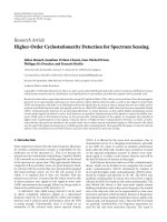
Ground truth event
Correctly detected event
Frame no

1400 2300 4250 4800
False alarm
1330 1500 2200 2770 4500 4800
1400 2570 4800 5200
4850
400 690 2320 3270
Figure 4: Detected events for i-LIDS datasets.
modeled as random variables. Using Bayesian theorem, joint
posterior density can be written as
p(μ, Σ
| X) ∝ p(X | μ, Σ)p(μ, Σ). (2)
To perform recursive Bayesian estimation with the new ob-
servations, joint prior density p(μ, Σ) should have the same
form with the joint posterior density p(μ, Σ
| X). Condition-
ing on the variance, joint prior density is written as
p(μ, Σ)
= p(μ | Σ)p(Σ). (3)
The above condition is realized if we assume inverse Wishart
distribution for the covariance and, conditioned on the co-
variance, multivariate normal distribution for the mean. In-
verse Wishart distribution is a multivariate generalization of
scaled inverse χ
2
-distribution. The parametrization is
Σ
∼Inv-Wishart
υ
t−1


Λ
−1
t
−1

,
μ
| Σ∼N

θ
t−1
,
Σ
κ
t−1

,
(4)
where υ
t−1
and Λ
t−1
are the degrees of freedom and scale ma-
trix for inverse Wishart distribution, θ
t−1
is the prior mean,
and κ
t−1
is the number of prior measurements. With these
assumptions, joint prior density becomes

p(μ, Σ)
∝|Σ|
−((υ
t−1
+3)/2+1)
× e
(−(1/2)tr(Λ
t−1
Σ
−1
)−(κ
t−1
)/2(μ−θ
t−1
)
T
Σ
−1
(μ−θ
t−1
))
(5)
for three-dimensional feature space. Let this density be la-
beled as normal inverse Wishart (θ
t−1
, Λ
t−1
/κ
t−1
; υ

t−1
, Λ
t−1
).
Multiplying prior density with the normal likelihood and ar-
ranging the terms, joint posterior density becomes normal
inverse Wishart (θ
t
, Λ
t
/κ
t
; υ
t
, Λ
t
) with the parameters up-
dated:
υ
t
= υ
t−1
+ nκ
n
= κ
t−1
+ n,
θ
t
= θ

t−1
κ
t−1
κ
t−1
+ n
+
x
n
κ
t−1
+ n
,
Λ
t
= Λ
t−1
+
n

i=1
(x
i
− x)(x
i
− x)
T
+ n
κ
t−1

κ
t
(x − θ
t−1
)(x − θ
t−1
)
T
,
(6)
where
x is the mean of new samples and n is the number of
samples used to update the model. If update is performed
at each time frame, n becomes one. To speed up the system,
update can be performed at regular time intervals by stor-
ing the observed samples. During our tests, we update one
quarter of the background at each time frame, therefore n
becomes four. The new parameters combine the prior in-
formation with the observed samples. Posterior mean θ
t
is
a weighted average of the prior mean and the sample mean.
The posterior degrees of freedom is equal to prior degrees of
freedom plus the sample size. System is started with the fol-
lowing initial parameters:
κ
0
= 10, υ
0
= 10, θ

0
= x
0
, Λ
0
= (υ
0
− 4)16
2
I,(7)
where I is the three-dimensional identity matrix.
Integrating joint posterior density with respect to Σ,we
get the marginal posterior density for the mean
p(μ
| X) ∝ t
υ
t
−2

μ | θ
t
,
Λ
t
κ
t

υ
t
− 2



,(8)
where t
υ
t
−2
is a multivariate t-distribution with υ
t
−2degrees
of freedom.
We use the expectations of marginal posterior distribu-
tions for mean and covariance as our model parameters at
6 EURASIP Journal on Advances in Signal Processing
Table 1: Detection results.
Sets T
all
T
event
Events TD FA T
true
T
miss
T
false
AB-easy 4850 2850 1 1 0 2220 630 0
AB-medium 4800 3000 1 1 1 1730 1270 970
AB-hard 5200 3400 1 1 1 2230 1170 350
PV-medium 3270 1920 1 1 0 1630 290 20
PETS 3000 1200 1 1 0 950 250 10

ATC-1 6600 3400 6 6 0 2350 1100 50
ATC-2 13500 6500 18 18 0 4740 1850 40
ATC-3 5700 2400 5 5 0 1390 1010 0
ATC-4 3700 2000 6 6 1 1300 700 350
ATC-5 9500 5350 11 10 2 3160 2150 420
time t. Expectation for marginal posterior mean (expectation
of multivariate t-distribution) becomes
μ
t
= E(μ | X) = θ
t
,(9)
whereas expectation of marginal posterior covariance (ex-
pectation of inverse Wishart distribution) becomes
Σ
t
= E(Σ | X) = (υ
t
− 4)
−1
Λ
t
. (10)
Our confidence measure for the layer is equal to one over
determinant of covariance of μ
| X:
C
=
1



Σ
μ|X


=
κ
3
t

υ
t
− 2

4

υ
t
− 4



Λ
t


. (11)
If our marginal posterior mean has larger variance, our
model becomes less confident. Note that variance of multi-
variate t-distribution with scale matrix Σ and degrees of free-

dom υ are equal to υ/(υ
− 2)Σ for υ>2.
System can be further speeded up by making indepen-
dence assumption on color channels. Update of full covari-
ance matrix requires computation of nine parameters. More-
over, during distance computation, we need to invert the full
covariance matrix. To speed up the system, we use three uni-
variate Gaussians corresponding to each color channel. After
updating each color channel independently, we join the vari-
ances and create a diagonal covariance matrix
Σ
t
=
⎛
⎜
⎝
σ
2
t,r
00
0 σ
2
t,g
0
00σ
2
t,b
⎞
⎟
⎠

. (12)
In this case, for each univariate Gaussian, we assume scaled
inverse χ
2
-distribution for the variance and conditioned on
the variance univariate normal distribution for the mean.
3.2. Background update
We initialize our system with k-layers for each pixel. Usually,
we select three-five layers. In more dynamic scenes, more lay-
ers are required. As we observe new samples for each pixel, we
update the parameters for our background model. We start
our update mechanism from the most confident layer in our
model. If the observed sample is inside the 99% confidence
interval of the current model, parameters of the model are
updated as explained in (6). Lower confidence models are not
updated.
For background modeling, it is useful to have a forgetting
mechanism so that the earlier observations have less effect on
the model. Forgetting is performed by reducing the number
of prior observation parameter of unmatched model. If cur-
rent sample is not inside the confidence interval, we update
the number of prior measurements parameter,
κ
t
= κ
t−1
− n, (13)
and proceed with the update of next confident layer. We do
not let κ
t

become less than initial value 10. If none of the
models is updated, we delete the least confident layer and ini-
tialize a new model having current sample as the mean and
an initial variance (7). The update algorithm for a single pixel
can be summarized as shown in Algorithm 1
With this mechanism, we do not deform our models with
noise or foreground pixels, but easily adapt to smooth inten-
sity changes like lighting effects. Embedded confidence score
determines the number of layers to be used and prevents un-
necessary layers. During our tests, usually secondary layers
correspond to shadowed form of the background pixel or dif-
ferent colors of the moving regions of the scene. If the scene
is unimodal, confidence scores of layers other than first layer
become very low.
3.3. Foreground segmentation
Learned background statistics are used to detect the changed
regions of the scene. We determine how many layers are nec-
essary for each pixel and use only those layers during fore-
ground segmentation phase. The number of layers required
to represent a pixel is not known beforehand, so background
is initialized with more layers than needed. Usually, we se-
lect three to five layers. In more dynamic scenes, more lay-
ers are required. Using the confidence scores, we determine
how many layers are significant for each pixel. As we observe
new samples for each pixel, we update the parameters for our
background model. At each update, at most one layer is up-
dated with the current observation. This assures the mini-
mum overlap over layers. We order the layers according to
Fatih Porikli et al. 7
1

(a)
1170
(b)
1750
(c)
Alarm!
2350
(d)
Alarm!
3000
(e)
Alarm!
3600
(f)
Alarm!
4130
(g)
Alarm!
4230
(h)
4300
(i)
4800
(j)
Figure 5: Test sequence AB-easy (Courtesy of i-LIDS). The alarm sets off immediately when the item is removed even though the luggage
was stationary 2000 frames (image size is 180
× 144).
1
(a)
200

(b)
300
(c)
400
(d)
500
(e)
600
Alarm!
(f)
640
Alarm!
(g)
700
Alarm!
(h)
720
(i)
750
(j)
Figure 6: In sequence ATC-2.2 (Courtesy of Advanced Technology Center, Amagasaki), one person brings a bag, puts it on the ground, another
person comes and picks it up. As visible, the object is detected accurately, and the alarm immediately sets off when the bag is removed.
confidence score and select the layers having confidence value
greater than the layer threshold. We refer to these layers as
confident layers. We start the update mechanism from the
most confident layer. If the observed sample is inside the 2.5σ
of the layer mean, which corresponds to 99% confidence in-
terval of the current model, parameters of the model are up-
dated. Lower confidence models are not updated.
4. EXPERIMENTAL RESULTS

To evaluate the dual foreground method, we used several
public datasets from PETS 2006, i-LIDS 2007, and Advanced
Technology Center. We tested a total of 32 sequences grouped
into 10 sets. The videos have assorted resolutions; 180
× 144,
320
× 240, and 640 × 480. The scenarios ranged from lunch
rooms to underground train stations. Half of these sequences
depict scenes that are not crowded. Other sequences con-
tain complex scenarios with multiple people sitting, stand-
ing, and walking at variable speeds. Some sequences show
vehicles parked. The abandoned items are left in different du-
rations from 10 seconds to 2 minutes. Some sequences con-
tained small abandoned items. A few sequences have multi-
ple abandoned items.
The sets AB-Easy, AB-Medium, and AB-Hard, which are
included in i-LIDS challenge, are recorded in an under-
ground train station. Set PETS is a large closed space plat-
form with restaurants. Sets ATC-1 and ATC-2 are recorded
from a wide angle camera of a cafeteria. Sets ATC-3 and
ATC-4 are different cameras from a lunch room. Set ATC-
5 is a waiting lounge. Since the proposed method is a pix-
elwise scheme, it is not difficult to set detection areas in
the initialization time. We manually marked the platform in
8 EURASIP Journal on Advances in Signal Processing
150
(a)
300
(b)
350

(c)
350
(d)
Alarm!
392
(e)
Alarm!
572
(f)
Alarm!
650
(g)
Alarm!
852
(h)
Alarm!
1050
(i)
1076
(j)
Figure 7: In sequence ATC-2.3 (Courtesy of Advanced Technology Center, Amagasaki), one person bring a bag, leaves it on the floor. As visible,
after it was detected as an abandoned item, temporary occlusions due to the moving people do not cause the system to fail.
120
(a)
200
(b)
250
(c)
268
(d)

300
(e)
Alarm!
550
(f)
Alarm!
614
(g)
Alarm!
700
(h)
724
(i)
770
(j)
Figure 8: In sequence ATC-2.6 (Courtesy of Advanced Technology Center, Amagasaki), one person hides the bag under a shadowed area of
the table and runs away. Another person comes, wanders around, takes the bag and leaves the scene.
AB-easy, AB-medium, and AB-hard sets, the waiting area in
PETS 2006 set, and the illegal parking spots in PV-easy, PV-
medium, and PV-hard sets. For the ATC sets, all of the image
area is used as the detection area. For i-LIDS sets, we replaced
the beginning parts of the video sequences with 4 frames of
the empty platform.
For all results, we set the learning rate of the short-term
background at 30 times the learning rate of the long-term
background. We assigned the evidence threshold max
e
in
the range [50, 500] depending on the desired responsiveness
time that controls how soon an abandoned item is detected

as an alarm. We used k
= 1 as the decay parameter.
Figure 4 shows the detection results for the i-LIDS
datasets. We reported the performance scores of all sets in
Ta ble 1,whereT
all
is the total number of frames in a set and
T
event
is the duration of the event in terms of the number of
frames. We measure the duration right after an item has been
left behind. It is also possible to measure the duration after
the person moved away or after some preset waiting time in
case additional tracking information is incorporated. Events
indicates the number of abandoned objects (for PV-medium,
the number of the illegally parked vehicles). TD means the
correctly detected objects. A detection event is considered to
be both spatially and temporally continuous. In other words,
there might be multiple detections for a frame if the ob-
jects are spatially disconnected. FA shows the falsely detected
objects. T
true
and T
false
are the duration of the correct and
false detections. T
miss
is the duration that an abandoned item
couldnotbedetected.Sincewestartaneventassoonasan
object is left, this score does not consider any waiting time.

This means that we overestimate our miss rate.
As our results show, we successfully detected almost all
abandoned items while achieving a very low false alarm rate.
Our method performed satisfactory when the initial frame
Fatih Porikli et al. 9
100
(a)
166
(b)
250
(c)
300
(d)
400
(e)
Alarm!
500
(f)
Alarm!
600
(g)
Alarm!
650
(h)
Alarm!
700
(i)
Alarm!
750
(j)

Figure 9: In sequence ATC-3.1 (Courtesy of Advanced Technology Center, Amagasaki), two people sit on a table. One person leaves a back
bag, another a bottle. They leave both items behind when they depart.
80
(a)
250
(b)
360
(c)
530
(d)
Alarm!
690
(e)
Alarm!
820
(f)
Alarm!
860
(g)
Alarm!
1000
(h)
Alarm!
1064
(i)
1118
(j)
Figure 10: In sequence ATC-5.3 (Courtesy of Advanced Technology Center, Amagasaki), one person sits on a couch and puts a bag next to
him. After a while, he leaves but the bag stays on the couch. Another person comes, sits on the couch, puts his briefcase next to him, and
takes away the bag. The briefcase is also removed later.

showed the actual static background. The detection areas
have not included any people at the initialization time in
the ATC sets, thus the uncontaminated backgrounds are eas-
ily learned. This is also true for the PV and AB-easy sets.
However, the AB-medium and AB-hard sets contained sev-
eral stationary people in the initial frames. This resulted in
false detections when those people moved away. Since the
background models eventually learn the statistically domi-
nant color values, such false alarms should not occur in the
long run due to the fact that the background will be more
visible than the people. In other words, the ratio of the false
alarms should decrease in time. We do not learn the color dis-
tribution of the abandoned items (or parked vehicles), thus
the proposed method can detect them even if they are oc-
cluded. As long as the occluding object, for example, a pass-
ing by person, has different color than the long-term back-
ground, our method still shows the boundary of the aban-
doned item.
Representative detection results are given in Figures 5–
12. As visible, none of the moving objects, moving shadows,
people that are stationary in shorter durations was falsely de-
tected. Besides, there are no ghost false detections due the
inaccurate blending of the abandoned items in the long-
term background. Thanks to the Bayesian update, the chang-
ing illumination conditions as in PV-medium are properly
adapted in the backgrounds.
Another advantage of this method is that the alarm is
immediately set of as soon as the abandoned item is re-
moved from its previous position. Although we do not know
whether the person who left the object is moved away from

the object or not, we consider this property as a superiority
over the tracking-based approaches that require a decision
10 EURASIP Journal on Advances in Signal Processing
600
(a)
900
(b)
1200
(c)
1500
(d)
1800
(e)
2100
(f)
2400
(g)
Alarm!
2800
(h)
Alarm!
2900
(i)
Alarm!
3000
(j)
Figure 11: A test sequence from PETS 2006 datasets (Courtesy of PETS). There is significant motion all around the scene. To make things
more challenging, the person who leaves his back bag after stays still for an extended period of time.
1
(a)

500
(b)
Alarm!
750
(c)
Alarm!
1250
(d)
Alarm!
1500
(e)
Alarm!
2000
(f)
Alarm!
2300
(g)
2350
(h)
2500
(i)
3000
(j)
Figure 12: Test sequence PV-medium from AVSS 2007 (Courtesy of i-LIDS). A challenge in this video is the rapidly changing illumination
conditions that cause dark shadows.
net of heuristic rules and context-depended priors to detect
such event.
One shortcoming is that it cannot discriminate the differ-
ent types of objects, for example, a person who is stationary
for a long time can be detected as an abandoned item. This

can be, however, an indication of another suspicious behav-
ior as it is not common. To determine object types and re-
duce the false alarm rate, object classifiers, that is, a human or
a vehicle detector, can be used. Since such classifiers are only
for verification purposes, their computation time should be
negligible. Since no tracking is integrated, trajectory-based
semantics, for example, who left the item or how long the
item left before the person moves away can not be extracted.
Still, our method can be used as a preprocessing stage to im-
prove the tracking-based video analytics.
The computational load of the proposed method is low.
Since we only employ pixelwise operations and make pixel-
wise decisions, we can take advantage of the parallel process-
ing architectures. By assigning each image pixel to a proces-
sor on the GPU using CUDA programming, since each pro-
cessor can execute in parallel, the speed improves more than
14
× in comparison to the corresponding CPU implementa-
tion. For instance, full background update for 360
× 288 im-
ages takes 74.32 milliseceonds on CPU (P4 DualCore 3GHz),
however on CUDA, it only needs 6.38 milliseceonds. We ob-
served that the detection can be comfortably employed in
quarter spatial resolution by processing the short-term back-
ground at 5 fps while updating the long term at every 5 sec-
onds (0.2 fps) with the same learning rates.
5. CONCLUSIONS
We present a robust method that uses dual foregrounds to
find abandoned items, stopped objects, and illegally parked
Fatih Porikli et al. 11

vehicles in static camera setups. At every frame, we adapt
the dual background models using Bayesian update, and ag-
gregate evidence obtained from dual foregrounds to achieve
temporal consistency.
This method does not depend on object initialization and
tracking of every single object, hence its performance is not
upper bounded to these error prone tasks that usually fail for
crowded scenes. It accurately outlines the boundary of items
even if they are fully occluded. Since it executes pixelwise op-
erations, it can be implemented on parallel processors.
ACKNOWLEDGMENT
The authors thank their colleagues Jay Thornton and Keisuke
Kojima for their constructive comments.
REFERENCES
[1] J. D. Courtney, “Automatic video indexing via object motion
analysis,” Pattern Recognition, vol. 30, no. 4, pp. 607–625, 1997.
[2] S. Velastin and A. Davies, “Intelligent CCTV surveillance: ad-
vances and limitations,” in Proceedings of the 5th International
Conference on Methods and Techniques in Behavioral Research,
Wageningen, The Netherlands, August-September 2005.
[3] A. E. Cetin, M. B. Akhan, B. U. Toreyin, and A. Aksay, “Char-
acterization of motion of moving objects in video,” US patent
no. 20040223652, 2004.
[4] H. Grabner and H. Bischof, “On-line boosting and vision,” in
Proceedings of IEEE Computer Society Conference on Computer
Vision and Pattern Recognition (CVPR ’06), vol. 1, pp. 260–267,
New York, NY, USA, June 2006.
[5] E. Auvinet, E. Grossmann, C. Rougier, M. Dahmane, and
J. Meunier, “Left-luggage detection using homographies and
simple heuristics,” in Proceedings of the 9th I EEE International

Workshop on Performance Evaluation in Tracking and Surveil-
lance (PETS ’06), pp. 51–58, New York, NY, USA, June 2006.
[6] J. Mart
´
ınez-del-Rinc
´
on, J. E. Herrero-Jaraba, J. R. G
´
omez,
and C. Orrite-Uru
˜
nuela, “Automatic left luggage detection
and tracking using multi-camera UKF,” in Proceedings of the
9th IEEE International Workshop on Performance Evaluation in
Tracking and Surveillance (PETS ’06), pp. 59–66, New York,
NY, USA, June 2006.
[7] N. Krahnstoever, P. Tu, T. Sebastian, A. Perera, and R. Collins,
“Multi-view detection and tracking of travelers and luggage
in mass transit environments,” in Proceedings of the 9th IEEE
International Workshop on Performance Evaluation in Tracking
and Surveillance (PETS ’06), pp. 67–74, New York, NY, USA,
June 2006.
[8] F. Lv, X. Song, B. Wu, V. K. Singh, and R. Nevatia, “Left lug-
gage detection using bayesian inference,” in Proceedings of the
9th IEEE International Workshop on Performance Evaluation in
Tracking and Surveillance (PETS ’06), pp. 83–90, New York,
NY, USA, June 2006.
[9] K. Smith, P. Quelhas, and D. Gatica-Perez, “Detecting aban-
doned luggage items in a public space,” in Proceedings of the
9th IEEE International Workshop on Performance Evaluation in

Tracking and Surveillance (PETS ’06), pp. 75–82, New York,
NY, USA, June 2006.
[10] S. Guler and M. K. Farrow, “Abandoned object detection in
crowded places,” in Proceedings of the 9th IEEE International
Workshop on Performance Evaluation in Tracking and Surveil-
lance (PETS ’06), pp. 99–106, New York, NY, USA, June 2006.
[11] C. StaufferandW.E.L.Grimson,“Adaptivebackgroundmix-
ture models for real-time tracking,” in Proceedings of the IEEE
Computer Society Conference on Computer Vision and Pattern
Recognition (CVPR ’99), vol. 2, pp. 246–252, Fort Collins,
Colo, USA, June 1999.
[12] F. Porikli and O. Tuzel, “Bayesian background modeling for
foreground detection,” in Proceedings of the 3rd ACM Inter-
national Workshop on Video Surveillance & Sensor Networks
(VSSN ’05), pp. 55–58, Singapore, November 2005.
[13] K. Toyama, J. Krumm, B. Brumitt, and B. Meyers, “Wallflower:
principles and practice of background maintenance,” in Pro-
ceedings of the 17th IEEE International Conference on Com-
puter Vision (ICCV ’99), vol. 1, pp. 255–261, Kerkyra, Greece,
September 1999.
[14] O. Javed, K. Shafique, and M. Shah, “A hierarchical approach
to robust background subtraction using color and gradient
information,” in Proceedings of the Workshop on Motion and
Video Computing (MOTION ’02), pp. 22–27, Orlando, Fla,
USA, December 2002.
[15] A. Mittal and N. Paragios, “Motion-based background sub-
traction using adaptive kernel density estimation,” in Proceed-
ings of the IEEE Computer Society Conference on Computer Vi-
sion and Pattern Recognition (CVPR ’04), vol. 2, pp. 302–309,
Washington, DC, USA, June-July 2004.

[16] A. Elgammal, D. Harwood, and L. Davis, “Non-parametric
model for background subtraction,” in Proceedings of the 6th
European Conference on Computer Vision-Part II (ECCV ’00),
vol. 2, pp. 751–767, Dublin, Ireland, June-July 2000.