Báo cáo hóa học: " Research Article Algorithms for Finding Small Attractors in Boolean Networks" potx

Hindawi Publishing Corporation
EURASIP Journal on Bioinformatics and Systems Biology
Volume 2007, Article ID 20180, 13 pages
doi:10.1155/2007/20180
Research Article
Algorithms for Finding Small Attractors in Boolean Networks
Shu-Qin Zhang,
1
Morihiro Hayashida,
2
Tatsuya Akutsu,
2
Wai-Ki Ching,
1
and Michael K. Ng
3
1
Advanced Modeling and Applied Computing Laboratory, Department of Mathematics, The University of Hong Kong,
Pokfulam Road, Hong Kong
2
Bioinformatics Center, Institute for Chemical Research, Kyoto University, Uji, Kyoto 611-0011, Japan
3
Department of Mathematics, Hong Kong Baptist University, Kowloon Tong, Hong Kong
Received 29 June 2006; Revised 24 November 2006; Accepted 13 February 2007
Recommended by Edward R. Dougherty
A Boolean network is a model used to study the interactions between different genes in genetic regulatory networks. In this paper,
we present several algorithms using gene ordering and feedback vertex sets to identify singleton attractors and small attractors in
Boolean networks. We analyze the average case time complexities of some of the proposed algorithms. For instance, it is shown that
the outdegree-based ordering algorithm for finding singleton attractors works in O(1.19
n
)timeforK = 2, which is much faster

than the naive O(2
n
) time algorithm, where n is the number of genes and K is the maximum indegree. We performed extensive
computational experiments on these algorithms, which resulted in good agreement with theoretical results. In contrast, we g ive a
simple and complete proof for showing that finding an attractor with the shortest period is NP-hard.
Copyright © 2007 Shu-Qin Zhang et al. This is an open access article distributed under the Creative Commons Attribution
License, which permits unrestricted use, distribution, and reproduction in any medium, provided the original work is properly
cited.
1. INTRODUCTION
The advent of DNA microarrays and oligonucleotide chips
has significantly sped up the systematic study of gene in-
teractions [1–4]. Based on microarray data, different kinds
of mathematical models and computational methods have
been developed, such as Bayesian networks, Boolean net-
works and probabilistic Boolean networks, ordinary and par-
tial differential equations, qualitative differential equations,
and other mathematical models [5]. Among all the models,
the Boolean network model has received much attention. It
was originally introduced by Kauffman [6–9]andreviews
can be found in [10–12]. In a Boolean network, gene ex-
pression states are quantized to only two levels: 1 (expressed)
and 0 (unexpressed). Although such binary expression is very
simple, it can retain meaningful biological information con-
tained in the real continuous-domain gene expression pro-
files. For instance, it can be applied to separation between
types of gliomas and types of sarcomas [13].
In a Boolean network, genes interact through some logi-
cal rules called Boolean functions. The state of a target gene is
determined by the states of its regulating genes (input genes)
and its Boolean function. Given the states of the input genes,

the Boolean funct ion transforms them into an output, which
is the state of the target gene. Although the Boolean network
model is very simple, its dynamic process is complex and can
yield insight to the global behavior of large genetic regulatory
networks [14].
The total number of possible global states for a Boolean
network with n genes is 2
n
. However, for any initial condi-
tion, the system will eventually evolve into a limited set of
stable states called attractors. The set of states that can lead
the system to a specific attractor is called the basin of attrac-
tion. There can be one or many states for each attractor. An
attractor having only one state is called a singleton attractor.
Otherwise, it is called a cyclic attractor.
There are two different interpretations for the function
of attractors. One intuition that follows Kauffman is that
one attractor should correspond to a cell type [11]. An-
other interpretation of attractors is that they correspond to
the cell states of growth, differentiation, and apoptosis [10].
Cyclic attractors should correspond to cell cycles (growth)
and singleton attractors should correspond to differentiated
or apoptosis states. These two interpretations are comple-
mentary since one cell type can consist of several neighboring
attractors and each of them corresponds to different cellular
functional states [15].
The number and length of attractors are important fea-
tures of networks. Extensive studies have been done for ana-
lyzing them. Starting from [11], a fast increase of the number
2 EURASIP Journal on Bioinformatics and Systems Biology

of attractors has been seen in [16–19]. Many studies have also
been done on the mean length of attractors [11, 17], although
there is no conclusive result.
It is also important to identify attractors of a given
Boolean network. In particular, identification of all singleton
attractors is important because singleton attractors corre-
spond to steady states in Boolean networks and have close re-
lation with steady states in other mathematical models of bi-
ological networks [10, 20–23]. As mentioned before, Huang
wrote that singleton attractors correspond to differentiation
and apoptosis states of a cell [10]. Devloo et al. transforms
the problem of finding steady states for some types of biolog-
ical networks to a constraint satisfaction problem [20]. The
resulting constraint satisfaction problem is very close to the
problem of identification of singleton attractors in Boolean
networks. Mochizuki introduced a general model of genetic
networks based on nonlinear differential equations [21]. He
analyzed the number of steady states in that model, where
steady states are again closely related to singleton attractors in
Boolean networks. Zhou et al. proposed a Bayesian-based ap-
proach to constructing probabilistic genetic networks [23].
Pal et al. proposed algorithms for generating Boolean net-
works with a prescribed attractor structure [22]. These stud-
ies focus on singleton attractors and it is mentioned that real-
world attractors are most likely to be singleton attractors,
rather than cyclic attractors.
Therefore, it is meaningful to identify singleton attrac-
tors. Of course, these can be done by examining all possible
states of a Boolean network. However, it would be too time
consuming even for small n, since 2

n
stateshavetobeex-
amined. Of course, if we want to find any one (not necessar-
ily singleton) attractor, we may find it by following the tra-
jectory to the attractor beginning from a randomly selected
state. If the basin of attraction is large, the possibility to find
the corresponding attractor would be high. However, it is not
guaranteed that a singleton attractor can be found. In order
to find a singleton attr actor, a lot of trajectories may be ex-
amined. Indeed, Akutsu et al. proved in 1998 that finding a
singleton attractor is NP-hard [24]. Independently, Milano
and Roli showed in 2000 that the satisfiability problem can be
transformed into the problem of finding a singleton attractor
[25], which provides a proof of NP-hardness of the singleton
attractor problem. Thus, it is not plausible that the singleton
attractor problem can be solved efficiently (i.e., polynomial
time) in all cases. However, it may be possible to develop al-
gorithms that are fast in practice and/or in the average case.
Therefore, this paper studies algorithms for identifying sin-
gleton attractors that are fast in many practical cases and have
concrete theoretical backg rounds.
Some studies have been done on fast identification of sin-
gleton attractors. Akutsu et al. proposed an algorithm for
finding singleton attractors based on a feedback vertex set
[24]. Devloo et al. proposed algorithms for finding steady
states of various biological networks using constraint pro-
gramming [20], which can also be applied to identification
of singleton attractors in Boolean networks. In particular, the
algorithms proposed by Devloo et al. are efficient in practice.
However, there are no theoretical results on the efficiency of

their algorithms. Thus, we aim at developing algor ithms that
are fast in practice and have a theoretical guarantee on their
efficiency (more precisely, the average case time complexity).
In this paper, we propose several algorithms for identify-
ing all singleton attractors. We first present a basic recursive
algorithm. In this algorithm, a partial solution is extended
one by one according to a given gene ordering that leads to
a complete solution. If it is found that a par tial solution can-
not be extended to a complete solution, the next partial solu-
tion is examined. This algorithm is quite similar to the back-
tracking method employed in [20]. The important differenc e
of this paper from [20] is that we perform some theoretical
analysis of the average case time complexity. For example, we
show that the basic recursive algorithm works in O(1.23
n
)
time in the average case under the condition that Boolean
networks with maximum indegree 2 are given uniformly at
random. It should be noted that O(1.23
n
)ismuchsmaller
than O(2
n
), though it is not polynomial.
Next, we develop improved algorithms using the out-
degree-based ordering and the breadth-first search (BFS)
based ordering. For these algorithms, we perform theoreti-
cal analysis of the average case time complexity, which shows
that these are better than the basic recursive algorithm.
Moreover, we examine the algorithm based on feedback ver-

tex sets (FVS) and its combination with the outdegree-based
ordering, where the idea of use of FVS was previously pro-
posed in our previous work [24]. We also perform computa-
tional experiments using these algorithms, which show that
the FVS-based algorithm with the outdegree-based gene or-
dering is the most efficient in practice among these algo-
rithms. Then, we extend the gene-ordering-based algorithms
for finding cyclic attractors with short periods along with
theoretical analysis and computational experiments. Though
we do not have strong evidence that small attractors are more
important than those with long periods, it seems that cell cy-
cles correspond to small attractors and large attractors are
not so common (with the exception of c ircadian rhythms)
in real biological networks. As a minimum, these extensions
show that application of the proposed techniques is not lim-
ited to the singleton attractor problem.
As mentioned before, NP-hardness results on finding a
singleton attractor (or the smallest attractor) were already
presented in [24, 25]. However, both papers appeared as con-
ference papers, the detailed proof is not given in [24], and the
transformation given in [25]isabitcomplicated.Therefore,
we describe a simple and complete proof. We believe that it is
worthy to include a simple and complete proof in this paper.
Finally, we conclude with future work.
2. ANALYSIS OF ALGORITHMS USING GENE
ORDERING FOR FINDING SINGLETON
ATTRACTORS
In this section, we present algorithms using gene ordering
for identification of singleton attractors along with theoreti-
cal analysis of the average case time complexity. Experimen-

tal results will be given later along with those of FVS-based
Shu-Qin Zhang et al. 3
Table 1: Example of a truth table of a Boolean network.
v
1
v
2
v
3
f
1
f
2
f
3
00 0 011
00 1
101
01 0
110
01 1
011
10 0
010
10 1
100
11 0
101
11 1
110

methods. Before presenting the algorithms, we briefly review
the Boolean network model.
2.1. Boolean network and attractor
A Boolean network G(V , F) consists of a set of n nodes (ver-
tices) V and n Boolean functions F,where
V
=

v
1
, v
2
, , v
n

,
F
=

f
1
, f
2
, , f
n

.
(1)
In general, V and F correspond to a set of genes and a set
of gene regulatory rules, respectively. Let v

i
(t) represent the
state of v
i
at time t. The overall expression level of all the
genes in the network at time step t is given by the following
vector:
v(t)
=

v
1
(t), v
2
(t), , v
n
(t)

. (2)
This vector is referred to as the Gene Activity Profile (GAP)
of the network at time t,wherev
i
(t) = 0 means that the
ith gene is not expressed and v
i
(t) = 1 means that it is ex-
pressed. Since v(t) ranges from [0, 0, , 0] (all entries are 0)
to [1, 1, , 1] (all entries are 1), there are 2
n
possible states.

The regulatory rules among the genes are given as follow:
v
i
(t +1)= f
i

v
i
1
(t), v
i
2
(t), , v
i
k
i
(t)

, i = 1, 2, , n. (3)
This ru le means that the state of gene v
i
at time t + 1 depends
on the states of k
i
genesattimet,wherek
i
is called the inde-
gree of gene v
i
. The maximum indegree of a Boolean network

is defined as
K
= max
i

k
i

. (4)
The number of genes that are directly affected by gene v
i
is called the outdegree of gene v
i
. The states of all genes
are updated synchronously according to the corresponding
Boolean functions.
A consecutive sequence of GAPs v(t), v(t +1), , v(t+ p)
is called an attractor with period p if v(t)
= v(t + p). An
attractor with period 1 is called a singleton attractor and an
attractor with p eriod > 1iscalledacyclic attractor.
Tab le 1 gives an example of a truth table of a Boolean net-
work. Each gene w ill update its state according to the states
of some other genes in the previous step. The state transi-
tions of this Boolean network can be seen in Figure 1.The
000 001
011 101
100 110
010 111
Figure 1: State transitions of the Boolean network shown in

Tabl e 1.
Input: a Boolean network G(V, F)
Output: all the singleton attractors
Initialize m :
= 1;
Procedure IdentSingletonAttractor(v, m)
if m
= n +1then Output v
1
(t), v
2
(t), , v
n
(t), return;
for b
= 0 to 1 do v
m
(t):= b;
if it is found that v
j
(t +1)=v
j
(t)forsome j≤m then
continue;
else IdentSingletonAttractor(v, m +1);
return.
Algorithm 1
system will eventually evolve into two attractors. One attrac-
tor is [0, 1, 1], which is a singleton attractor, and the other
one is

[1,0,1]
−→ [1,0,0] −→ [0,1,0]−→ [1,1,0]−→ [1,0,1],
(5)
which is a cyclic att ractor with period 4.
2.2. Basic recursive algorithm
The number of singleton attractors in a Boolean network de-
pends on the regulatory rules of the network. If the regula-
tory rules are given as v
i
(t +1)= v
i
(t)foralli, the number of
singleton attractors is 2
n
. Thus, it would take O(2
n
)timein
the worst case if we want to identify all the singleton attrac-
tors. On the other hand, it is known that the average number
of singleton attractors is 1 regardless of the number of genes
n and the maximum indegree K [21]. Therefore, it is useful
to develop algorithms for identifying all singleton attractors
without examining all 2
n
states ( in the average case).
For that purpose, we propose a very simple algorithm,
whichisreferredtoasthebasic recursive algorithm in this pa-
per. In the algorithm, a partial GAP (i.e., profile with m (<n)
genes) is extended one by one towards a complete GAP (i.e.,
4 EURASIP Journal on Bioinformatics and Systems Biology

singleton attractor), according to a given gene ordering. If it
is found that a partial GAP cannot be extended to a singleton
attractor, the next partial GAP is examined. The pseudocode
of the algorithm is given as shown in Algorithm 1.
The algorithm extends a partial GAP by one gene at a
time. At the mth recursive step, the states of the first m
− 1
genes are determined. Then, the algorithm extends the par-
tial GAP by a dding v
m
(t) = 0. If v
j
(t +1)= v
j
(t) holds or the
value of v
j
(t + 1) is not determined for all j = 1, , m, the
algorithm proceeds to the next recursive step. That is, if there
is a possibility that the current partial GAP can be extended
to a singleton attractor, it goes to the next recursive step.
Otherwise, it extends the partial GAP by adding v
m
(t) = 1
and executes a similar procedure. After examining v
m
(t) = 0
and v
m
(t) = 1, the algorithm returns to the previous recur-

sive step. Since the number of singleton attractors is small in
most cases, it is expected that the algorithm does not exam-
ine many partial GAPs with large m. The average case time
complexity is estimated as follows.
Suppose that Boolean networks with maximum indegree
K aregivenuniformlyatrandom.Thentheaveragecasetime
complexity of the algorithm for K
= 1 to K = 10 isgiveninthe
first row of Ta bl e 2 .
Theoretical analysis
Assume that we have tested the first m out of n genes, where
m
≥ K.Foralli ≤ m, v
i
(t) = v
i
(t + 1) holds with probability
P

v
i
(t) = v
i
(t +1)

=
0.5 ·

m
C

k
i
n
C
k
i

≈
0.5 ·

m
n

k
i
≥ 0.5 ·

m
n

K
.
(6)
If v
i
(t) = v
i
(t + 1) does not hold, the algorithm can continue.
Therefore, the probability that the algorithm examines the
(m +1)thgeneisnotmorethan


1 − P

v
i
(t) = v
i
(t +1)

m
=

1 − 0.5 ·

m
n

K

m
. (7)
Thus, the number of recursive calls executed for the first m
genes is at most
f (m)
= 2
m
·

1 − 0.5 ·


m
n

K

m
. (8)
Let s
= m/n,and f (s) = [2
s
· (1 − 0.5 · s
K
)
s
]
n
= [(2 − s
K
)
s
]
n
.
The average case time complexity is estimated by the maxi-
mum value of f (s). Though an additional O(nm)factorisre-
quired, it can be ignored since O(n
2
a
n
)  O((a + )

n
)holds
for any a>1and
 > 0.
Since the time complexity should be a function with re-
spect to n, we only need to compute the maximum value of
the function g(s)
= (2 − s
K
)
s
. With simple numerical cal-
culations, we can get its maximum value for fixed K.Then,
the average case time complexity of the algorithm can be es-
timated as O((max(g))
n
). We list the time complexity from
K
= 1 to 10 in the first row of Ta ble 2.AsK gets larger, the
complexity increases.
2.3. Outdegree-based ordering algorithm
In the basic recursive algorithm, the original ordering of
genes was used. If we sort the genes according to their out-
degree (genes are ordered from larger outdegree to smaller
outdegree),itisexpectedthatvaluesofv
j
(t +1)foralarger
number of genes are determined at each recursive step than
those determined for the basic recursive algorithm, and thus
a lower number of partial GAPs are examined. This intuition

is justified by the following theoretical analysis.
Suppose that Boolean networks with maximum indegree K
are given uniformly at random. After reordering all genes ac-
cording to their outdegrees from largest to smallest, the average
case time complexity of the algorithm for K
= 1 to K = 10 is
given in the second row of Tabl e 2 .
Theoretical analysis
We assume (without loss of generality) w.l.o.g. that the inde-
grees of all genes are K. If the input genes for any gene are
randomly selec ted from all the genes, the outdegree of genes
follows the Poisson distribution with mean approximately λ.
In this case, λ
= K holds since the total indegree must be
equal to the total outdegree. Thus, λ and K are confused in
the following. The probability that a gene has outdegree k is
P(k)
=
λ
k
exp(−λ)
k!
. (9)
We reorder the genes according to their outdegrees from
largest to smallest. Assume that the first m genes have been
tested and gene m is the uth gene among the genes with out-
degree l. Then
m
− u = n ·
∞


k=l+1
λ
k
exp(−λ)
k!
(10)
and therefore
n
− m = n ·
l

k=0
λ
k
exp(−λ)
k!
− u. (11)
The total outdegree of these n
− m genes is
n
·
l

k=0
λ
k
exp(−λ)
k!
· k − u · l. (12)

The total outdegree for the first m genes is
λn
−

n ·
l

k=0
λ
k
exp(−λ)
k!
· k − u · l

=
λn − λn ·
l−1

k=0
λ
k
exp(−λ)
k!
+ u
· l
= λn − λ

n − (m − u) − n ·
λ
l

exp(−λ)
l!

+ u · l
= λm + λn ·
λ
l
exp(−λ)
l!
+ u(l
− λ).
(13)
Shu-Qin Zhang et al. 5
Thus, for i ≤ m,wehave
P

v
i
(t) = v
i
(t +1)

=
0.5 ·

λm + λn ·

λ
l
exp(−λ)/l!


+ u(l − λ)
λn

λ
= 0.5 ·

m
n
+
λ
l
exp(−λ)
l!
+
(l
− λ)u
λn

λ
.
(14)
The number of recursive calls executed for the first m genes
is
f (m)
= 2
m
·

1 − 0.5 ·


m
n
+
λ
l
exp(−λ)
l!
+
(l
− λ)u
λn

λ

m
.
(15)
Letting s
= m/n, f (m)canberewrittenas
f (m)
=

2
s
·

1 − 0.5 ·

s +

λ
l
exp(−λ)
l!
+
(l
− λ)u
λn

λ

s

n
=

2 −

s +
λ
l
exp(−λ)
l!
+
(l
− λ)u
λn

λ


s

n
.
(16)
As in Section 2.2, we estimate the maximum value of g(s)
where it is defined here as g(s)
= [2 − (s + λ
l
exp(−λ)/l!+
(l
− λ)u/λn)
λ
]
s
. We also must consider the relationship be-
tween l and λ.
(1) If l>λ,
g(s)
≤

2 −

s +
λ
l
exp(−λ)
l!

λ


s
= g
1
(s). (17)
Since λ
l
exp(−λ)/l! tends to zero if l is large, we only
need to examine several small values of l. The upper
bound of g(s) can be obtained by computing the max-
imum value of g
1
(s) with some numerical methods.
However, we should be careful so that
P(k
≥ l +1)≤ s ≤ P(k ≥ l) (18)
holds. That is, it should be guaranteed that the maxi-
mum value obtained is for the gene with outdegree l.
(2) If l
= λ,
g(s)
=

2 −

s +
λ
l
exp(−λ)
l!


λ

s
. (19)
Similar to above, we can get an upper bound for g(s).
(3) If l<λ,
g(s)
=

2 −

s +
λ
l
exp(−λ)
l!
+
(l
− λ)u
λn

λ

s
. (20)
Since gene m is the uth gene among the genes with out-
degree l,
u
≤ n ·

λ
l
exp(−λ)
l!
. (21)
Thus,
g(s)
≤

2 −

s +
λ
l
exp(−λ)
l!
+
(l
− λ)
λn
· n ·
λ
l
exp(−λ)
l!

λ

s
=


2 −

s +
λ
l
exp(−λ)
l!
+(l
− λ) ·
λ
l−1
exp(−λ)
l!

λ

s
.
(22)
There are only a few values that are less than λ. Using a
method similar to the one above, we can get an upper
bound for g(s).
It should be noted that l must belong to exactly one of these
three cases when g(s) reaches its maximum value. Summa-
rizing the three different cases above, we can get an approxi-
mation of the average case time complexity of the algorithm.
The second row of Tabl e 2 shows the time complexity of the
algorithm for K
= 1toK = 10. As in Section 2.2, the com-

plexity increases as K increases.
We remark that the difference between this improved al-
gorithm and the basic recursive algorithm lies only in that we
need to sort all the genes according to their outdegrees from
largest to smallest before executing the main procedure of the
basic recursive algorithm.
2.4. Breadth-first search-based
ordering algorithm
Breadth-first search is a general technique for traversing a
graph. It v isits all the nodes and edges of a graph in a man-
ner that all the nodes at depth (distance from the root node)
d are visited before visiting nodes at depth d +1.Forexam-
ple, suppose that node a hasoutgoingedgestonodesb and
c, b has outgoing edges to nodes d and e,andc has outgo-
ing edges to nodes f and g, where other edges (e.g., an edge
from d to f ) can exist. In this case, nodes are visited in the
order of a, b, c, d, e, f . In this way, all of the nodes are to-
tally ordered according to the visiting order. The algorithm
for implementing BFS can be found in many text books. The
computation time for BFS on a graph with n nodes and m
edges is O(n+m). If we use this BFS-based ordering, as in the
case of outdegree-based ordering, it is expected that values of
v
j
(t +1)foralargernumberofgenesaredeterminedateach
recursive step, and thus, lower numbers of partial GAPs are
examined. We can estimate the average case time complexity
as follows.
Suppose that Boolean networks with maximum indegree K
are given uniformly at random. After reordering all genes ac-

cording to the BFS-ordering, the average case time complexity
of the algorithm for K
= 1 to K = 10 is given in the third row
of Ta ble 2.
Theoretical analysis
As in Section 2.3, we assume w.l.o.g. that all n genes have
the same indegree K. Suppose that we have tested m genes.
Since the input genes of the ith gene must be among the first
K
· i + 1 genes, whether v
i
(t +1) = v
i
(t)ornotcanbede-
termined before visiting the (K
· i + 2)th gene. According to
6 EURASIP Journal on Bioinformatics and Systems Biology
Table 2: Theoretical time complexities of basic, outdegree-based, and BFS-based algorithms.
K 1 2345678910
Basic 1.23
n
1.35
n
1.43
n
1.49
n
1.53
n
1.57

n
1.60
n
1.62
n
1.65
n
1.67
n
Outdegree-based 1.09
n
1.19
n
1.27
n
1.34
n
1.41
n
1.45
n
1.48
n
1.51
n
1.56
n
1.57
n
BFS-based ≈ O(n)1.16

n
1.27
n
1.35
n
1.41
n
1.45
n
1.50
n
1.53
n
1.56
n
1.58
n
the determination pattern of states of m genes, we consider 3
cases.
(1) The states of the first (m
− 1)/K genes are deter-
mined and they must satisfy v
i
(t+1) = v
i
(t), where a
denotes the standard floor function. Then, we have
P

v

i
(t) = v
i+1
(t)

=
0.5, i ≤ 
m
− 1
K
. (23)
(2) For any gene i between the m/Kth gene and the
(n
− 1)/Kth gene, whether v
i
(t +1)isequaltov
i
(t)
can be determined before examining the (m + j
· K)th
gene, where j
= 1, 2, , (n − m)/K. Then, we have
P

v
i
(t) = v
i+1
(t)


=
0.5 ·

m
m + j · K

K
,

m
K

≤ i ≤

n
− 1
K

.
(24)
The algorithm can continue for any gene i with prob-
ability
1
− P

v
i
(t) = v
i+1
(t)


=
1 − 0.5 ·

m
m + j · K

K
,

m
K

≤ i ≤

n
− 1
K
.
(25)
(3) From the n/Kth gene to the mth gene, the input
genes to them can be any gene; thus
P

v
i
(t) = v
i+1
(t)


= 0.5 ·

m
n

K
, 
n
− 1
K

≤ i ≤ m. (26)
Here, the algorithm can continue for each gene with
probability
1
−P

v
i
(t) = v
i+1
(t)

=
1 − 0.5 ·

m
n

K

, 
n
− 1
K

≤ i ≤ m.
(27)
The probability that the algorithm can be executed for all
m genes is

(m−1)/K

i=1
P

v
i
(t) = v
i+1
(t)


·

(n−1)/K

i=(m−1)/K

1 − P


v
i
(t) = v
i+1
(t)


·

m

i=(n−1)/K

1 − P

v
i
(t) = v
i+1
(t)


=
0.5
(m−1)/K
·

(n−1)/K

i=(m−1)/K


1−0.5 ·

m
m + i · K

K

·

1 − 0.5 ·

m
n

K

m−(n−1)/K

.
(28)
Then, the total number of recursive calls is
f (m)
= 2
m
· 0.5
(m−1)/K
·

(n−1)/K


i=(m−1)/K

1 − 0.5 ·

m
m + i · K

K

·

1 − 0.5 ·

m
n

K

m−(n−1)/K

≤
2
m
· 0.5
(m−1)/K
·

1 − 0.5 ·


m
n

K

m−(m−1)/K
=

2 −

m
n

K

m−(m−1)/K
=

2 −

m
n

K

[(m−(m−1)/K)/n]·n
≈

2 −


m
n

K

(m/n)(1−1/K)·n
.
(29)
Let s
= m/n and g(s) = (2 − s
K
)
s(1−1/K)
. Using numerical
methods, we can get the maximum value of g.FromK
= 1to
K
= 10, the upper bound of the average case time complexity
of the algorithm is in the third row of Tab le 2 .
It is to be noted that in the estimation of the upper bound
of f (m), we overestimated the probability that genes belong
to the second case, and thus the upper b ound obtained here is
not tight. More accurate time complexities can be estimated
from the results of computational experiments.
Shu-Qin Zhang et al. 7
3. FINDING SINGLETON ATTRACTORS USING
FEEDBACK VERTEX SET
In this section, we present algorithms based on the feedback
vertex set and the results of computational experiments on
all of our proposed algorithms for identification of singleton

attractors. The algorithms in this section are based on a sim-
ple and interesting property on acyclic Boolean networks al-
though they can be applied to general Boolean networks with
cycles. Though an algorithm based on the feedback vertex set
was already proposed in our previous work [24], some im-
provements (ordering based on connected components and
ordering based on outdegree) are achieved in this section.
3.1. Acyclic network
As to be shown in Section 5, the problem of finding a single-
ton attractor in a Boolean network is NP-hard. However, we
have a positive result for acyclic networks as fol lows.
Proposition 1. If the network is acyclic, there exists a unique
singleton attractor. Moreover, the unique attractor can be com-
puted in polynomial time.
Proof. In an acyclic network, there exists at least one node
without incoming edges. Such nodes should have fixed
Boolean values. The values of the other nodes are uniquely
determined from these nodes by the nth time step in polyno-
mial time. Since the state of any node does not change after
the nth step, there exists only one singleton attrac tor.
As shown below, this property is also useful for identify-
ing singleton attrac tors in cyclic networks.
3.2. Algorithm
In the basic recursive algorithm, we must consider truth as-
signments to all the nodes in the network. On the other
hand, Proposition 1 indicates that if the network is acyclic,
the truth values of all nodes are uniquely determined from
the values of the nodes with no incoming edges. Thus, it is
enough to examine truth assignments only to the nodes with
no incoming edges, if we can decompose the network into

acyclic graphs. Such a set of nodes is called a feedback vertex
set (FVS). The problem of finding a minimum feedback ver-
tex set is known to be NP-hard [26]. Some algorithms which
approximate the minimum feedback vertex set have been de-
veloped [27]. However, such algorithms are usually compli-
cated. Thus, we use a simple greedy algorithm (shown in
Algorithm 2) for finding a (not necessarily minimum) feed-
back vertex set, where a similar algorithm was already pre-
sented in [24]. In our proposed algorithm, nodes in FVS are
ordered according to the connected components of the orig-
inal network in order to reduce the number of iterations. In
other words, nodes in the same connected component are
ordered sequentially.
Then, we modify the procedure IdentSingletonAttrac-
tor(v, m) for FVS as shown in Algorithm 3.
Input: a Boolean network G(V, F)
Output: an ordered feedback vertex set F
=

v
(FVS)
1
, , v
(FVS)
M

Procedure FindFeedbackVertexSet
let F :
= ∅, M := 1;
let C:

= (all the connected components of G);
for each connected component C

∈ C do
let V

:= (a set of vertices in C

);
while V

=∅do
let v
(FVS)
M
:= (a vertex selected randomly from V

);
remove v
(FVS)
M
and vertices whose truth values
can be fixed only from F in V

;
increment M.
Algorithm 2
Input: a Boolean network G(V, F) and an ordered feedback
vertex set F
=


v
(FVS)
1
, , v
(FVS)
M

Output: all the singleton attractors
Initialize m :
= 1;
Procedure IdentSingletonAttractorWithFVS(v, m)
if m
= M +1then Output v
1
(t), v
2
(t), , v
n
(t), return;
for b
= 0 to 1 do v
(FVS)
m
(t):= b;
propagate truth values of

v
(FVS)
1

(t), , v
(FVS)
m
(t)

to
all possible v(t)exceptF ;
compute

v
(FVS)
1
(t +1), , v
(FVS)
m
(t +1)

from v(t);
if it is found that v
(FVS)
j
(t +1)= v
(FVS)
j
(t)forsome
j
≤ m then
continue;
else IdentSingletonAttractorWithFVS(v, m +1);
return.

Algorithm 3
Furthermore, we can combine the outdegree-based or-
dering with FVS. In FindFeedbackVertexSet, we select a node
randomly from a connected component. When combined
with the outdegree-based ordering, we can instead select the
node with the maximum outdegree in a connected compo-
nent.
3.3. Computational experiments
In this section, we evaluate the proposed algorithms by per-
forming a number of computational experiments on both
random networks and scale-free networks [28].
3.3.1. Experiments on random networks
For each K (K
= 1, , 10) and each n (n = 1, , 20),
we randomly generated 10 000 Boolean networks with max-
imum indegree K and took the average values. All of these
computational experiments were done on a PC with Opteron
8 EURASIP Journal on Bioinformatics and Systems Biology
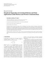
Table 3: Empirical time complexities of basic, outdegree, BFS, feedback vertex set, and FVS + outdegree algorithms.
K 12345678910
Basic 1.27
n
1.39
n
1.46
n
1.53
n
1.57
n

1.60
n
1.63
n
1.67
n
1.69
n
1.70
n
Outdegree 1.14
n
1.23
n
1.30
n
1.37
n
1.42
n
1.47
n
1.51
n
1.54
n
1.56
n
1.59
n

BFS 1.09
n
1.16
n
1.24
n
1.31
n
1.37
n
1.42
n
1.45
n
1.49
n
1.52
n
1.53
n
Feedback 1.10
n
1.28
n
1.39
n
1.47
n
1.53
n

1.56
n
1.60
n
1.64
n
1.66
n
1.68
n
FVS + Outdegree 1.05
n
1.13
n
1.21
n
1.29
n
1.35
n
1.41
n
1.46
n
1.49
n
1.52
n
1.55
n

1
1.1
1.2
1.3
1.4
1.5
1.6
1.7
Base of the time complexity (a of a
n
)
12345678910
Indegree K
Basic
Outdegree
BFS
Feedback
FVS + outdegree
Figure 2: Base of the empirical time complexity (a
n
’s a value) of the
proposed algorithms for finding singleton attractors.
2.4 GHz CPUs and 4 GB RAM running under the Linux (ver-
sion 2.6.9) operating system, where the gcc compiler (version
3.4.5) was used with optimization option -O3.
Tab le 3 shows the empirical time complexity of each pro-
posed method for each K. We used a tool for GNUPLOT to fit
the function b
· a
n

to the experimental results. The tool uses
the nonlinear least-squares (NLLS) Marquardt-Levenberg al-
gorithm. Figure 2 is a graphical representation of the result
of Ta ble 3. It is seen that the FVS + Outdegree method is the
fastest in most cases.
Figure 3 is an example to show the average number of
iterations with respect to the number of genes for K
= 2.
Figure 4 shows the average computation time with respect to
the number of genes when K
= 2, where similar results were
obtained for other values of K.
The time complexities estimated from the results of com-
putational experiments are a little different from those ob-
tained by theoretical analysis. However, this is reasonable
since, in our theoretical analysis, we assumed that the num-
ber of genes is very large, we made some approximations,
and there were also small numerical errors in computing the
maximum values of g(s).
1
10
100
1000
10000
The number of iterations
2 3 4 5 6 7 8 9 10 11 12 13 14 15 16 17 18 19 20
The number of nodes
Basic O(1.39
n
)

Outdegree O(1.23
n
)
BFS O(1.16
n
)
Feedback O(1.28
n
)
FVS + outdegree O(1.13
n
)
Figure 3: Number of iterations done by the proposed algorithms
for K
= 2.
3.3.2. Experiments on scale-free networks
It is known that many real biological networks have the scale-
free property (i.e., the degree distribution approximately fol-
lows a power-law) [28]. Furthermore, it is observed that in
gene regulatory networks, the outdegree distribution follows
a power-law and the indeg ree distribution follows a Poisson
distribution [29]. Thus, we examined networks with scale
free topology.
We generated scale-free networks with a power-law out-
degree dist ribution (
∝ k
−2
) and a Poisson indegree distribu-
tion (with the average indegree 2) as follows. We first choose
the number of outputs for each gene from a power-law dis-

tribution. That is, gene v
i
has L
i
outputs where all the L
i
are
drawn from a power-law distribution. Then, we choose the L
i
outputs of each gene v
i
randomly with uniform probability
from n genes. Once each gene has been assigned with a set of
outputs, the inputs of all genes are fully determined because
v
j
is an input of v
i
if v
i
is an output of v
j
. Since L
i
output
genes are chosen randomly for each gene v
i
, the indegree dis-
tribution should follow a Poisson distribution.
Figure 5 compares the outdegree-based algorithm, the

BFS-based algorithm and the FVS + Outdegree algorithm for
scale-free networks generated as above and for random net-
works with constant indegree 2, where the average CPU time
Shu-Qin Zhang et al. 9
1e-06
1e-05
1e-04
0.001
0.01
Elapsed time (s)
2 3 4 5 6 7 8 9 10 11 12 13 14 15 16 17 18 19 20
The number of nodes
Basic
Outdegree
BFS
Feedback
FVS + outdegree
Figure 4: Elapsed time (in seconds) by the proposed algorithms for
random networks with K
= 2.
1e-05
1e-04
0.001
0.01
0.1
1
10
100
1000
Elapsed time (s)

40 50 60 70 80 90 100 110 120
The number of nodes
Fix/outdegree
Fix/BFS
Fix/FVS + outdegree
PS/outdegree
PS/BFS
PS/FVS + outdegree
Figure 5: Elapsed time (in seconds) of some of the proposed algo-
rithms for random networks with K
= 2 (Fix) and scale-free net-
works (PS).
was taken over 100 networks for each case and a PC with
Xeon 5160 3 GHz CPUs with 8 GB RAM was used. The result
is interesting and we observed that all algorithms work much
faster for scale-free networks than for random networks. This
result is reasonable because scale-free networks have a much
larger number of high degree nodes than random networks
and thus heuristics based on the outdegree-based ordering
or the BFS-based ordering should work efficiently. The aver-
age case time complexities estimated from this experimen-
tal result are as follows: O(1.19
n
)versusO(1.09
n
) for the
outdegree-based algorithm, O(1.12
n
)versusO(1.09
n

) for the
Input: a Boolean network G(V, F) and a period p
Output: all of the small attractors with period p
Initialize m :
= 1;
Procedure IdentSmallA ttractor(v, m)
if m
= n +1then Output v
1
(t), v
2
(t), , v
n
(t), return;
for b
= 0 to 1 do v
m
(t):= b;
for p

=0 to p−1 do compute v(t+p

+1) from v(t+p

);
if it is found that v
j
(t+p)=v
j
(t)forsome j ≤m then

continue;
else IdentSmallAttractor( v, m +1);
return.
Algorithm 4
BFS-based algorithm, and O(1.12
n
)versusO(1.05
n
) for the
FVS + Outdegree algorithm, where (random) versus (scale-
free) is shown for each case. The average case complexities
for random networks are better than those in Tabl e 3 and are
closer to the theoretical time complexities shown in Ta ble 2.
These results are reasonable because networks with much
larger number of nodes were examined in this case.
It should be noted that Devloo et al. proposed constraint
programming based methods for finding steady-states in
some kinds of biological networks [20]. Their methods use a
backtracking technique, which is very close to our proposed
recursive algorithms, and may also be applied to Boolean net-
works. Their methods were applied to networks up to several
thousand nodes with indegree
= outdegree = 2. Since differ-
ent types of networks were used, our proposed methods can-
not be directly compared with their methods. Their methods
include various heuristics and may be more useful i n practice
than our proposed methods. However, no theoretical analy-
sis was performed on the computational complexity of their
methods.
4. FINDING SMALL ATTRACTORS

In this sec tion, we modify the gene-ordering-based algo-
rithms presented in Section 2 to find cyclic attractors with
short periods. We also perform a theoretical analysis and
computational experiments.
4.1. Modifications of algorithms
The basic idea of our modifications is very simple. Instead
of checking whether or not v
i
(t +1)= v
i
(t)holds,wecheck
whether or not v
i
(t + p) = v
i
(t) holds. The pseudocode of the
modified basic recursive algorithm is given in Algorithm 4.
This procedure computes v(t + p) from the truth assign-
ments on the first m genes of v(t). Values of some genes of
v(t + p) may not be determined because these genes may also
depend on the last (n
− m)genesofv(t). If either v
j
(t + p) =
v
j
(t) holds or the value of v
j
(t + p) is not determined for
each j

= 1, , m, the algorithm will continue to the next
10 EURASIP Journal on Bioinformatics and Systems Biology
recursive step. As in Section 2, we can combine this algorithm
with the outdegree-based ordering and the BFS-based order-
ing.
In these algorithms, it is assumed that the period p is
given in advance. However, the algorithms can be modified
for identifying all cyclic attractors with period at most P.For
that purpose, we simply need to execute the algorithms for
each of p
= 1, 2, , P. Though this method does not seem to
be practical, its theoretical time complexity is still better than
O(2
n
) for small P. Suppose that the average case time com-
plexity for p is O(T
p
(n)). Then, this simple method would
take O(

P
p
=1
T
p
(n)) ≤ O(P · T
P
(n)) time, which is stil l faster
than O(2
n

)ifT
P
(n) = o(2
n
)andP is bounded by some poly-
nomial of n.
4.2. Theoretical analysis
Before giving the experimental results, we perform a theoret-
ical analysis on the modified basic recursive algorithm.
Suppose that Boolean networks with maximum indegree
K aregivenuniformlyatrandom.Thentheaveragecasetime
complexity of the modified basic recursive algorithm for pe riod
1 to 5 and K
= 1 to K = 10 is given in Ta bl e 4 .
Theoretical analysis
Let the period of the attr actor be p. We assume w.l.o.g. as
before that the indegree of all genes is K.AsinSection 2.2,
we consider the first m genes among all n genes. Given the
states of all m genes at time t, we need to know the states of all
these genes at time t + p. The probability that v
i
(t) = v
i
(t + p)
holds for each i
≤ m is approximated by:
P

v
i

(t) = v
i
(t + p)

=
0.5 ·

m
n

K
·

m
n

K
2
···

m
n

K
p
,
(30)
where (m/n)
K
means that the K input genes to gene v

i
at time
t + p
− 1 are among the first m genes, (m/n)
K
2
means that at
time t + p
− 2 the input genes to the K input genes to gene v
i
are also in the first m genes, and so on.
Then, the probability that the algorithm examines some
specific truth assignment on m genes is approximately given
by

1 − P

v
i
(t) = v
i
(t + p)

m
=

1 − 0.5 ·

m
n


K
·

m
n

K
2
···

m
n

K
p

m
.
(31)
Therefore, the number of total recursive calls executed for
these m genes is
f (m)
= 2
m
·

1 − P

v

i
(t) = v
i
(t + p)

m
= 2
m
·

1 − 0.5 ·

m
n

K
·

m
n

K
2
···

m
n

K
p


m
.
(32)
As in Section 2.2, we can compute the maximum value of
f (m).TheresultsaregiveninTabl e 4.
1
1.1
1.2
1.3
1.4
1.5
1.6
1.7
1.8
1.9
2
Base of the time complexity (a of a
n
)
12345678910
Indegree K
Basic
Outdegree
BFS
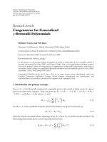
Figure 6: Base of the empirical time complexity (a
n
’s a value) of the
proposed algorithms for finding cyclic attractors with period 2.
1.1

1.2
1.3
1.4
1.5
1.6
1.7
1.8
1.9
2
Base of the time complexity (a of a
n
)
12345678910
Indegree K
Basic
Outdegree
BFS
Figure 7: Base of the empirical time complexity (a
n
’s a value) of the
proposed algorithms for finding cyclic attractors with period 3.
4.3. Computational experiments
Computational experiments were also performed to exam-
ine the time complexity of the algorithms for finding small
attractors. The environment and parameters of the experi-
ments were the same as in Section 3.3.1. Though FVS-based
algorithms can also be modified for small attractors, they are
not efficient for p>1. Therefore, we only examined gene-
ordering-based algorithms.
Figures 6 to 8 show the time complexity of the algorithms

estimated from the results of computational experiments for
p
= 2top = 4andforK = 1toK = 10. When K is com-
paratively small, the outdegree-based ordering method is the
Shu-Qin Zhang et al. 11
Table 4: Theoretical time complexities for the modified basic algorithm for finding small attractors with period p.
K 12345678910
p = 1 1.23
n
1.35
n
1.43
n
1.49
n
1.53
n
1.57
n
1.60
n
1.62
n
1.65
n
1.67
n
p = 2 1.35
n
1.57

n
1.70
n
1.78
n
1.83
n
1.87
n
1.89
n
1.91
n
1.92
n
1.93
n
p = 3 1.43
n
1.72
n
1.86
n
1.92
n
1.95
n
1.97
n
1.97

n
1.98
n
1.99
n
1.99
n
p = 4 1.49
n
1.83
n
1.94
n
1.97
n
1.99
n
1.99
n
1.99
n
1.99
n
1.99
n
1.99
n
p = 5 1.53
n
1.90

n
1.97
n
1.99
n
1.99
n
1.99
n
1.99
n
1.99
n
1.99
n
1.99
n
1.1
1.2
1.3
1.4
1.5
1.6
1.7
1.8
1.9
2
Base of the time complexity (a of a
n
)

12345678910
Indegree K
Basic
Outdegree
BFS
Figure 8: Base of the time complexity (a
n
’s a value) of the proposed
algorithms for finding cyclic attractors with period 4.
most efficient. But when K increases, all the three methods
perform the same, w hich is equivalent to the worst case in
finding the attrac tors, that is O(2
n
). The results obtained
from the numerical experiments for the modified basic re-
cursive algorithm are consistent with the theoretical results
presented in Section 4.2 .
5. HARDNESS RESULT
As mentioned in Section 1, Akutsu et al. [24] and Milano and
Roli [25] showed that finding a singleton attractor (or an at-
tractor with the shortest period) is NP-hard. Those results
justify our proposed algorithms which take exponential time
in the worst case (and even in the average case). However,
the proof is omitted in [24] and the proof in [25]isabit
complicated: Boolean functions assigned in the transformed
Boolean network are much longer than those in the original
satisfiability problem. Here we give a simpler and complete
proof.
Theorem 1. Finding an attractor with the shortest pe riod is
NP-hard.

Proof. We show that deciding whether or not there exists a
singleton attractor is NP-hard, from which the theorem fol-
lows since the singleton attractor is the attractor with the
shortest per iod (if any such period exists).
We use a simple polynomial time reduction from 3SAT
[26] to the singleton attractor problem.
Let x
1
, , x
N
be Boolean var iables (i.e., 0-1 variables).
Let c
1
, , c
L
be a set of clauses over x
1
, , x
N
,whereeach
clause is a logical OR of at most three literals. It should be
noted that a literal is a variable or its negation (logical NOT).
Then, 3SAT is a problem of asking whether or not there exists
an assignment of 0-1 values to x
1
, , x
N
which satisfies all
the clauses (i.e., the values of all clauses are 1).
From an instance of 3SAT, we construct an instance of the

singleton attractor problem. We let the set of vertices (nodes)
V
={v
1
, , v
N+L
},whereeachv
i
for i = 1, , N corre-
sponds to x
i
and each v
N+i
for i = 1, , L corresponds to c
i
.
For each v
i
such that i ≤ N, we make the following assign-
ment:
v
i
(t +1)= v
i
(t). (33)
Suppose that f
i
(x
i
1

, , x
i
3
)isaBooleanfunctionassignedto
c
i
in 3SAT. Then, for each v
N+i
, we assign the following func-
tion:
v
N+i
(t +1)= f
i

v
i
1
(t), v
i
2
(t), v
i
3
(t)

∨
v
N+i
(t). (34)

Figure 9 is an example of reduction from 3SAT to the single-
ton attractor problem.
Here, we show that 3SAT is satisfiable if and only if there
exists a singleton attractor.
Suppose that there exists an assignment of Boolean values
b
1
, , b
N
to x
1
, , x
N
which satisfies all clauses c
1
, , c
L
.
Then, we let
v
i
(0) =
⎧
⎨
⎩
b
i
for i = 1, , N,
1fori
= N +1, , N + L.

(35)
It is straight forward to see that v(0)
= (v
1
(0), , v
N+L
(0)) is
a singleton attractor (i.e., v(0)
= v(1)).
Suppose that there exists a singleton a ttractor. Let v(0)
=
(v
1
(0), , v
N+L
(0)) be the state of the singleton attractor.
Then, v
N+i
(0) must be 1 for all i = 1, , L. Otherwise
(i.e., v
N+i
(0) = 0), v
N+i
(1) would be 1 and it contradicts
the assumption that v(0) is a singleton attractor. Further-
more, f
i
(v
i
1

(0), v
i
2
(0), v
i
3
(0)) = 1 must hold. Otherwise,
v
N+i
(1) would be 0 since the equations v
N+i
(0) = 1and
f
i
(v
i
1
(0), v
i
2
(0), v
i
3
(0)) = 0 hold. This contradicts the as-
sumption that v(0) is a singleton attractor. Therefore, by as-
signing v
i
(0) to x
i
for i = 1, , N, all the clauses are satisfied.

Since the reduction can trivially be done in polynomial
time, we have the theorem.
12 EURASIP Journal on Bioinformatics and Systems Biology
v
1
v
2
v
3
v
4
v
5
v
6
v
7
v
1
v
2
v
3
v
5
v
1
v
3
v

4
v
6
v
2
v
3
v
4
v
7
Figure 9: Example of a reduction from 3SAT to the singleton at-
tractor problem. An instance of 3SAT
{x
1
∨ x
2
∨ x
3
, x
1
∨ x
3
∨ x
4
, x
2
∨
x
3

∨ x
4
} is transformed into this Boolean network.
6. CONCLUSION
In this paper, we have presented fast algorithms for identify-
ing singleton attractors and cyclic attractors with short peri-
ods. The proposed algorithms are much faster than the naive
enumeration-based algorithm. However, the proposed algo-
rithms cannot be applied to random networks with several
hundreds or more genes. Moreover, it may not be faster than
the constraint programming-based algorithms in [20]. How-
ever, the most important point of this work is that the aver-
age case time complexities of the ordering-based algorithms
are analyzed and are shown to be better than O(2
n
). We hope
that our work stimulates further development of faster algo-
rithms and deeper theoretical analysis.
It is interesting that the results of computational experi-
ments suggest that our proposed algorithms are much faster
for scale-free networks than for random networks. However,
we could not yet perform theoretical analysis for scale-free
networks. Thus, theoretical analysis of the average c ase time
complexity for scale-free networks (precisely, networks with
a power-law outdegree distribution and a Poisson indegree
distribution) is left as future work.
Although this paper focused on the Boolean network as a
model of biological networks, the techniques proposed here
may be useful for designing algorithms for finding steady
states in other models and for theoretical analysis of such

algorithms. For instance, Mochizuki performed theoretical
analysis on the number of steady states in some continu-
ous biological networks that are based on nonlinear differ-
ential equations [21]. However, the core part of the analysis
is done in a combinatorial manner and is very close to that
for Boolean networks. Thus, it may be possible to develop
fast algorithms for finding steady states in such continuous
network models. Application and extension of the proposed
techniques to other types of biological networks are impor-
tant future research topics.
Finally, it is interesting to compare the complexities of
four problems for three classes of networks: simulation of
network behavior (almost trivial), identification of attr actors
(this paper), identification of networks [30, 31], and find-
ing control strategies [32] for trees, acyclic graphs, and gen-
eral graphs. These four problems constitute a more com-
plete picture of modeling genetic regulatory networks with
Table 5: Comparison of time complexities for simulation of net-
work behavior, identification of attractors, finding control strate-
gies, and identification of networks. P means that the problem can
be solved in polynomial time.
Tree
Acyclic
graph
General
graph
Simulation of network PPP
Identification of attractor
PPNP-hard
Finding control strategies

P NP-hard NP-hard
Identification of network
NP-hard NP-hard NP-hard
Identification of network
(bounded indegree)
PPP
a Boolean network. Simulation of a Boolean network is a
trivial but important step to analyze the model. Attractors
describe the long run behavior of the Boolean network sys-
tem. Finding a control strategy is to consider how the sys-
tem can be made to evolve desirably. Identification of genetic
regulatory networks is the first step in obtaining the model
from data. Tabl e 5 shows complexities for various problems
with several network structures. Although many works have
been done for these problems, the computational complex-
ity is still an important issue. It is also left as future work to
study how to cope with high computational complexity (e.g.,
NP-hardness) of these problems.
ACKNOWLEDGMENTS
We thank anonymous reviewers for helpful comments. TA
was partially supported by a Grant-in-Aid “Systems Ge-
nomics” from MEXT, Japan and by the Cel l Arr ay Project
from NEDO, Japan. WKC was partially supported by Hung
Hing Ying Physical Research Fund, HKU GRCC Grants nos.
10206647, 10206483, and 10206147. MKN was partially sup-
ported by RGC 7046/03P, 7035/04P, 7035/05P, and HKBU
FRGs. S Q. Zhang and M. Hayashida contributed equally to
this work.
REFERENCES
[1]J.E.Celis,M.Kruhøffer,I.Gromova,etal.,“Geneexpres-

sion profiling: monitoring transcription and tr anslation prod-
ucts using DNA microarrays and proteomics,” FEBS Letters,
vol. 480, no. 1, pp. 2–16, 2000.
[2] T. R. Hughes, M. Mao, A. R. Jones, et al., “Expression profil-
ing using microarrays fabricated by an ink-jet oligonucleotide
synthesizer,” Nature Biotechnology, vol. 19, no. 4, pp. 342–347,
2001.
[3] R. J. Lipshutz, S. P. A. Fodor, T. R. Gingeras, and D. J. Lock-
hart, “High density synthetic oligonucleotide arrays,” Nature
Genetics, vol. 21, supplement 1, pp. 20–24, 1999.
[4] D. J. Lockhart and E. A. Winzeler, “Genomics, gene expres-
sion and DNA arrays,” Nature, vol. 405, no. 6788, pp. 827–836,
2000.
[5] H. D. Jong, “Modeling and simulation of genetic regulatory
systems: a literature review,” Journal of Computational Biology,
vol. 9, no. 1, pp. 67–103, 2002.
Shu-Qin Zhang et al. 13
[6] K.GlassandS.A.Kauffman, “The logical analysis of continu-
ous, nonlinear biochemical control networks,” Journal of The-
oretical Biology, vol. 39, no. 1, pp. 103–129, 1973.
[7] S. A. Kauffman, “Metabolic stability and epigenesis in ran-
domly constructed genetic nets,” Journal of Theoretical Biology,
vol. 22, no. 3, pp. 437–467, 1969.
[8] S.A.Kauffman, “Homeostasis and differentiation in random
genetic control networks,” Nature, vol. 224, no. 215, pp. 177–
178, 1969.
[9] S.A.Kauffman, “The large scale structure and dynamics of ge-
netic control circuits: an ensemble approach,” Journal of The-
oretical Biology, vol. 44, no. 1, pp. 167–190, 1974.
[10] S. Huang, “Gene expression profiling, genetic networks, and

cellular states: an integrating concept for tumorigenesis and
drug discovery,” Journal of Molecular Medicine, vol. 77, no. 6,
pp. 469–480, 1999.
[11] S. A. Kauffman, The Origins of Order: Self-Organization and
Selection in Evolution, Oxford University Press, New York, NY,
USA, 1993.
[12] R. Somogyi and C. Sniegoski, “Modeling the complexity of ge-
netic networks: understanding multigenic and pleiotropic reg-
ulation,” Complexity, vol. 1, no. 6, pp. 45–63, 1996.
[13] I. Shmulevich and W. Zhang, “Binary analysis and
optimization-based normalization of gene expression
data,” Bioinformatics, vol. 18, no. 4, pp. 555–565, 2002.
[14] D. Thieffry,A.M.Huerta,E.P
´
erez-Rueda, and J. Collado-
Vides, “From specific gene regulation to genomic networks:
a global analysis of transcriptional regulation in Escherichia
coli,” BioEssays, vol. 20, no. 5, pp. 433–440, 1998.
[15] S. Huang, “Cell state dynamics and tumorigenesis in
Boolean regulatory networks,” InterJournal Genetics, MS: 416,
/>[16] B. Drossel, “Number of attractors in random Boolean net-
works,” Physical Review E, vol. 72, no. 1, Article ID 016110,
5 pages, 2005.
[17] B. Drossel, T. Mihaljev, and F. Greil, “Number and length of at-
tractors in a critical Kauffman model with connectivity one,”
Physical Rev i ew Letters, vol. 94, no. 8, Article ID 088701, 4
pages, 2005.
[18] B. Samuelsson and C. Troein, “Superpolynomial growth in the
number of attractors in Kauffman networks,” Physical Rev iew
Letters, vol. 90, no. 9, Article ID 098701, 4 pages, 2003.

[19] J. E. S. Socolar and S. A. Kauffman, “Scaling in ordered and
critical random Boolean networks,” Physical Review Letters,
vol. 90, no. 6, Article ID 068702, 4 pages, 2003.
[20] V. Devloo, P. Hansen, and M. Labb
´
e, “Identification of all
steady states in large networks by logical analysis,” Bulletin of
Mathematical Biology, vol. 65, no. 6, pp. 1025–1051, 2003.
[21] A. Mochizuki, “An analytical study of the number of steady
states in gene regulatory networks,” Journal of Theoretical Bi-
ology, vol. 236, no. 3, pp. 291–310, 2005.
[22] R. Pal, I. Ivanov, A. Datta, M. L. Bittner, and E. R. Dougherty,
“Generating Boolean networks with a prescribed attractor
structure,” Bioinformatics, vol. 21, no. 21, pp. 4021–4025,
2005.
[23]X.Zhou,X.Wang,R.Pal,I.Ivanov,M.Bittner,andE.R.
Dougher ty, “A Bayesian connectivity-based approach to con-
structing probabilistic gene regulatory networks,” Bioinfor-
matics, vol. 20, no. 17, pp. 2918–2927, 2004.
[24] T. Akutsu, S. Kuhara, O. Maruyama, and S. Miyano, “A system
for identifying genetic networks from gene expression patterns
produced by gene disruptions and overexpressions,” Genome
Informatics, vol. 9, pp. 151–160, 1998.
[25] M. Milano and A. Roli, “Solving the s atisfiability problem
through B oolean networks,” in Proceedings of the 6th Congress
of the Italian Association for Artificial Intelligence on Advances
in Artificial Intelligence, vol. 1792 of Lecture Notes in Artifi-
cial Intelligence, pp. 72–83, Springer, Bologna, Italy, September
1999.
[26] M. R. Garey and D. S. Johnson, Computers and Intractability: A

Guide to the Theory of NP-Completeness, W.H. Freeman, New
York, NY, USA, 1979.
[27] G. Even, J. Naor, B. Schieber, and M. Sudan, “Approximating
minimum feedback sets and multicuts in directed graphs,” Al-
gorithmica, vol. 20, no. 2, pp. 151–174, 1998.
[28] A L. Barab
´
asi and R. Albert, “Emergence of scaling in random
networks,” Science, vol. 286, no. 5439, pp. 509–512, 1999.
[29] N. Guelzim, S. Bottani, P. Bourgine, and F. K
´
ep
`
es, “Topologi-
cal and causal structure of the yeast transcriptional regulatory
network,” Nature Genetics, vol. 31, no. 1, pp. 60–63, 2002.
[30] T. Akutsu, S. Miyano, and S. Kuhara, “Identification of genetic
networks from a small number of gene expression patterns un-
der the Boolean network model,” in Proceedings of the 4th Pa-
cific Symposium on Biocomputing (PSB ’99), vol. 4, pp. 17–28,
Big Island of Hawaii, Hawaii, USA, January 1999.
[31] T. Akutsu, S. Kuhara, O. Maruyama, and S. Miyano, “Iden-
tification of genetic networks by strategic gene disruptions
and gene overexpressions under a B oolean model,” Theoreti-
cal Computer Science, vol. 298, no. 1, pp. 235–251, 2003.
[32] T. Akutsu, M. Hayashida, W K. Ching, and M. K. Ng, “Con-
trol of Boolean networks: hardness results and algorithms
for tree structured networks,” Journal of Theoretical Biology,
vol. 244, no. 4, pp. 670–679, 2007.