Báo cáo hóa học: " Research Article Detection-Guided Fast Affine Projection Channel Estimator for Speech Applications" potx

Hindawi Publishing Corporation
EURASIP Journal on Audio, Speech, and Music Processing
Volume 2007, Article ID 71495, 13 pages
doi:10.1155/2007/71495
Research Article
Detection-Guided Fast Affine Projection Channel Estimator for
Speech Applications
Yan Wu Jennifer,
1
John Homer,
2
Geert Rombouts,
3
and Marc Moonen
3
1
Canberra Research Laboratory, National ICT Australia and Research School of Information Science and Engineering,
The Australian National University, Canberra ACT 2612, Australia
2
School of Information Technology and Electrical Engineering, The University of Queensland, Brisbane QLD 4072, Australia
3
Departement Elektrotechniek, Katholieke Universiteit Leuven, ESAT/SCD, Kasteelpark Arenberg 10, 30001 Heverlee, Belgium
Received 9 July 2006; Revised 16 November 2006; Accepted 18 February 2007
Recommended by Kutluyil Dogancay
In various adaptive estimation applications, such as acoustic echo cancellation within teleconferencing systems, the input signal is
a highly correlated speech. This, in general, leads to extremely slow convergence of the NLMS adaptive FIR estimator. As a result,
for such applications, the affine projection algorithm (APA) or the low-complexity version, the fast affine projection (FAP) algo-
rithm, is commonly employed instead of the NLMS algorithm. In such applications, the signal propagation channel may have a
relatively low-dimensional impulse response structure, that is, the number m of active or significant taps within the (discrete-time
modelled) channel impulse response is much less than the overall tap length n of the channel impulse response. For such cases, we
investigate the inclusion of an active-parameter detection-guided concept within the fast affine projection FIR channel estimator.

Simulation results indicate that the proposed detection-guided fast affine projection channel estimator has improved convergence
speed and has lead to better steady-state perfor mance than the standard fast affine projection channel estimator, especially in the
important case of highly correlated speech input signals.
Copyright © 2007 Yan Wu Jennifer et al. This is an open access article distributed under the Creative Commons Attribution
License, which permits unrestricted use, dist ribution, and reproduction in any medium, provided the original work is properly
cited.
1. INTRODUCTION
For many adaptive estimation applications, such as acous-
tic echo cancellation within teleconferencing systems, the in-
put signal is highly correlated speech. For such applications,
the standard normalized least-mean square (NLMS) adaptive
FIR estimator suffers from extremely slow convergence. The
use of the affine projection algorithm (APA) [1] is considered
as a modification to the standard NLMS estimators to greatly
reduce this weakness. The built-in prewhitening properties
of the APA greatly accelerate the convergence speed especially
with highly correlated input signals. However, this comes
with a significant increase in the computational cost. The
lower complexity version of the APA, the fast affine pro-
jection (FAP) algorithm, which is functionally equivalent to
APA, was introduced in [2].
The fast affine projection algorithm (FAP) is now, per-
haps, the most commonly implemented adaptive algorithm
for high correlation input signal applications.
For the above-mentioned applications, the sig nal prop-
agation channels being estimated may have a “low dimen-
sional” parametric representation [3–5]. For example, the
impulse responses of many acoustic echo paths and com-
munication channels have a “small” number m of “active”
(nonzero response) “taps” in comparison with the overall

tap length n of the adaptive FIR estimator. Conventionally,
estimation of such low-dimensional channels is conducted
using a standard FIR filter with the nor malized least-mean
square (NLMS) adaptive algorithm (or the unnormalized
LMS equivalent). In these approaches, each and every FIR
filter tap is NLMS-adapted during each time interval, which
leads to relatively slow convergence r a tes and/or relatively
poor steady-state performance. An alternative approach pro-
posed by Homer et al. [6–8]istodetectandNLMSadapt
only the active or significant filter taps. The hypothesis is that
this can lead to improved convergence rates and/or steady-
state performance.
Motivated by this, we propose the incorporation of an
activity detection technique within the fast affine projec-
tion FIR channel estimator. Simulation results of the new ly
proposed detection-guided fast affine projection channel
2 EURASIP Journal on Audio, Speech, and Music Processing
estimator demonstra te faster convergence and better steady-
state error performance over the standard FAP FIR channel
estimator, especially in the important case of highly corre-
lated input signals such as speech. These features make this
newly proposed detection-guided FAP channel estimator a
good candidate for adaptive channel estimation applications
such as acoustic echo cancellation, where the input signal is
highly correlated speech and the channel impulse response is
often “long” but “low dimensional.”
The remainder of the paper is set out as follows. In Sec-
tion 2 we provide a description of the adaptive system we
consider throughout the paper as well as the affine projec-
tion algorithm (APA) [1] and the fast affine projection algo-

rithm (FAP) [2]. Section 3 begins with a brief overview of the
previous proposed detection-guided NLMS FIR estimators
of [6–8]. We then propose our detection-guided fast affine
projection FIR channel estimator. Simulation conditions are
presented in Section 4, followed by the simulation results in
Section 5. The simulation results include a comparison of our
newly proposed estimator with the standard NLMS chan-
nel estimator, the earlier proposed detection-guided NLMS
channel estimator [8], the standard APA channel estimator
[1] as well as the standard FAP channel estimator [2]in3
different input correlation level cases.
2. SYSTEM DESCRIPTION
2.1. Adaptive estimator
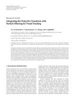
We consider the adaptive FIR channel estimation system of
Figure 1. The following assumptions are made:
(1) al l the signals are sampled: at sample instant k, u(k)
is the signal input to the unknown channel and the
channel estimator; additive noise v(k) occurs within
the unknown channel;
(2) the unknown channel is linear and is adequately mod-
elled by a discrete-time FIR filter Θ
= [θ
0
, θ
1
, , θ
n
]
T
with a maximum delay of n sample intervals;

(3) the additive noise signal is zero mean and uncorrelated
with the input signal;
(4) the FIR-modeled unknown channel, Θ[z
−1
]issparsely
active:
Θ

z
−1

= θ
t
1
z
−t
1
+ θ
t
2
z
−t
2
+ ···+ θ
t
m
z
−t
m
,(1)

where m
 n,and0≤ t
1
<t
2
< ···t
m
≤ n.
At sample instant k,anactive tap is defined as a tap cor-
responding to one of the m indices
{t
a
}
m
a
=1
of (1). Each of the
remaining taps is defined as an inactive tap.
The observed output from the unknown channel is
y(k)
= Θ
T
U(k)+v(k), (2)
where U
(k) = [u(k), u(k − 1), , u(k − n)]
T
.
u(k)
Channel
v(k)

y(k)
+
−
Adaptive estimator
y(k)
e(k)
Figure 1: Adaptive channel estimator.
The standard adaptive NLMS estimator equation, as em-
ployed to provide an estimate

θ of the unknown channel
impulse response vector Θ, is as follows [9]:

θ(k +1)=

θ(k)+
μ
U
T
(k)U(k)+δ
U
(k)

y(k) − y(k)

,
(3)
where
y(k) =


θ
T
(k)U(k)andwhereδ is a small positive reg-
ularization constant.
Note: the standard initial channel estimate

θ(0) is the all-
zero vector.
For stable 1st-order mean behavior, the step size μ should
satisfy 0 <μ
≤ 2. In practice, however, to attain higher-order
stable behavior, the step size is chosen to satisfy 0 <μ
 2.
For the standard discrete NLMS a daptive FIR estimator,
every coefficient

θ
i
(k)[i = 0, 1, , n]isadaptedateachsam-
ple interval. However, this approach leads to slow conver-
gence rates when the required FIR filter tap length n is “large”
[6]. In [6–8], it is shown that if only the active or significant
channel taps are NLMS estimated then the convergence rate
of the NLMS estimator may be greatly enhanced, particularly
when m
 n.
2.2. Affine projection algorithm
The affine projection algorithm (APA) is considered as a gen-
eralisation of the normalized least-mean-square (NLMS) al-
gorithm [2]. Alternatively, the APA can be viewed as an in-

between solution to the NLMS and R LS algorithms in terms
of computational complexity and convergence rate [10]. The
NLMS algorithm updates the estimator taps/weights on the
basis of a single-input vector, which can be viewed as a one-
dimensional affine projection [11]. In APA, the projections
are made in multiple dimensions. The convergence rate of
the estimator’s tap weight vector greatly increases with an in-
crease in the projection dimension. This is due to the built-in
decorrelation properties of the APA.
To describe the affine projection algorithm (APA) [1], the
following notations are defined:
Yan Wu Jennifer et al. 3
(a) N:affine projection order;
(b) n + 1: length of the adaptive channel estimator
excitation signal matrix of size (n+1)
×N;
(c) U(k): U(k)
= [U(k), U(k − 1), ,
U
(k − (N − 1))], where
U
(k) = [u(k), u(k − 1), , u(k − n)]
T
;
(d) U
T
(k)U(k): covariance matrix;
(e) Θ: the channel FIR tap weight vector, where
Θ
= [θ

0
, θ
1
, , θ
n
]
T
;
(f)

θ(k): the adaptive estimator FIR tap
weight vector at sample instant k where

θ(k) = [

θ
0
(k),

θ
1
(k), ,

θ
n
(k)]
T
;
(g)


θ(0): initial channel estimate with the al l-zero
vector;
(h) e
(k): the channel estimation signal error vector
of length N;
(i) ε
(k): N-length normalized residual estimation
error vector;
(j) y( k): system output;
(k) v(k): the additive system noise;
(l) δ: regularization parameter;
(m) μ: step size par ameter.
The affine projection algorithm can be described by the
following equations (see Figure 1).
The system output y(k) involves the channel impulse re-
sponse to the excitation/input and the additive system noise
v(k) and is given by (2).
The channel estimation signal error vector e
(k)iscalcu-
lated as
e
(k) = Y (k) − U(k)
T

θ(k − 1), (4)
where Y (k)
= [y(k), y(k − 1), , y(k − N +1)]
T
.
The normalized residual channel estimation error vector

ε
(k), is calculated in the following way:
ε
(k) =

U(k)
T
− U(k)+δI

−1
· e(k), (5)
where I
= N × N identity matrix.
The APA channel estimation vector is updated in the fol-
lowing way:

θ(k +1)=

θ(k)+μU(k)ε(k). (6)
A regularization term δ times the identity matrix is added
to the covariance matrix within (5) to prevent the insta-
bility problem of creating a singular matrix inverse when
[
U(k)
T
U(k)
] has eigenvalues close to zero. A well behaved
inverse will be provided if δ is large enough.
From the above equations, it is obvious that the relations
(4), (5), (6) reduce to the standard NLMS algorithm if N

= 1.
Hence, the affine projection algorithm (APA) is a generaliza-
tion of the NLMS algorithm.
2.3. Fast affine projection algorithm
The complexity of the APA is about 2(n +1)N +7N
2
,which
is generally much larger than the complexity of the NLMS
algorithm, 2(n + 1). Motivated by this, a fast version of the
APA was derived in [2]. Here, instead of calculating the error
vector from the whole covariance matrix, the FAP only cal-
culates the first element of the N-element error vector, where
an approximation is made for the second to the last compo-
nents of the error vector e
(k)as(1− μ) times the previously
computed error [12, 13]:
e
(k +1)=

e(k +1)
(1
− μ)e(k)

,(7)
where the N
− 1lengthe(k) consists of the N − 1upperele-
ments of the vector e
(k).
Note: (7) is an exact formula for the APA if and only if
δ

= 0.
The second complexity reduction is achieved by only
adding a weighted version of the last column of U(k)toup-
date the tap weight vector. Hence there are just (n +1)mul-
tiplications as opposed to N
× (n + 1) multiplications for the
APA update of (6). Here, an alternate tap weight vector

θ
1
(k)
is introduced.
Note: the subscript 1 denotes the new calculation meth-
od.

θ
1
(k +1)=

θ
1
(k) − μU(k − N +2)E
N−1
(k + 1), (8)
where
E
N−1
(k +1)=
N−1


j=0
ε
j
(k − N +2+j)
= ε
N−1
(k +1)+ε
N−2
(k)+···+ ε
0
(k − N +2)
(9)
is the (N
− 1)th element in the vector
E
(k +1)=
⎡
⎢
⎢
⎢
⎢
⎣
ε
0
(k +1)
ε
1
(k +1)+ε
0
(k)

.
.
.
ε
N−1
(k +1)+ε
N−2
(k)+···+ ε
0
(k − N +2)
⎤
⎥
⎥
⎥
⎥
⎦
.
(10)
Alternatively, E
(k +1)canbewrittenas
E
(k +1)=

0
E(k)

+ ε(k + 1), (11)
where
E(k)isanN − 1 length vector consisting of
the upper most N

− 1 elements of E(k)andε(k +
1)
= [ε
N−1
(k +1),ε
N−2
(k +1)+···+ ε
0
(k +1)]
T
as calcu-
lated via (5).
Hence, it can be shown that the relationship between the
new update method and the old update method of APA can
be viewed as

θ(k) =

θ
1
(k)+μU(k)E(k), (12)
where
U(k) consists of the N − 1 leftmost columns of U(k).
4 EURASIP Journal on Audio, Speech, and Music Processing
Anewefficient method to calculate e(k) using

θ
1
(k)
rather than


θ(k) is also derived:
r
xx
(k +1)= r
xx
(k)+u(k +1)α(k +1)− u(k − n)α(k − n),
(13)
where
α(k +1)=

u(k), u(k − 1), ,u(k − N +2)

T
(14)
e
1
(k +1)= y(k +1)− U(k +1)
T

θ
1
(k) (15)
e(k +1)
= e
1
(k +1)− μr
t
xx
(k +1)E(k). (16)

(Further details can be found in [2].)
The following is a summary of the FAP algorithm:
(1)
r
xx
(k+1) = r
xx
(k)+u(k+1)α(k+1)−u(k−n)α(k−n),
(2) e
1
(k +1)= y(k +1)− U(k +1)
T

θ
1
(k),
(3) e(k +1)
= e
1
(k +1)− μr
t
xx
(k +1)E(k),
(4) e
(k +1)=

e(k+1)
(1
−μ)e(k)


,
(5) ε
(k +1)= [U(k +1)
T
U(k +1)+δI]
−1
e(k +1),
(6) E
(k +1)=

0
E(k)

+ ε(k +1),
(7)

θ
1
(k +1)=

θ
1
(k) − μU(k − N +2)E
N−1
(k +1).
The above formulae are in general only approximately
equivalent to the APA; they are exactly equal to the APA if
the regularization δ is zero. Steps (2) and (7) of the FAP al-
gorithm are each of complexity (n + 1) MPSI (multiplica-
tions per symbol interval). Step (1) is of complexity 2N MPSI

and steps (3), (4), (6) are each of complexity N MPSI. Step
(5), when implemented in the Levinson-Dubin method, re-
quires 7N
2
MPSI [2]. Thus, the complexity of FAP is roughly
2(n +1)+7N
2
+5N. For many applications like echo cancel-
lation, the filter length (n + 1) is always much larger than the
required affine projection order N, which makes FAP’s com-
plexity comparable to that of NLMS. Furthermore, the FAP
only requires slightly more memory than the NLMS.
3. DETECTION-GUIDED ESTIMATION
3.1. Least-squares activity detection criteria review
The original least-squares-based detection criterion for iden-
tifying active FIR channel taps for white input signal condi-
tions [6] is as follows.
The tap index j is defined to be detected as a member of
the active tap set
{t
a
}
m
a
=1
at sample instant k if
X
j
(k) >T
(k)

, (17)
where
X
j
(k) =


k
i
=1

y(i)u(i − j)

2


k
i
=1
u
2
(i − j)
,
T(k)
=
2log(k)
k
k

i=1

y
2
(i).
(18)
However, the original least-square-based detection criterion
suffers from tap coupling problems when colored or corre-
lated input signals are applied. In particular, the input cor-
relation causes X
j
(k) to depend not only on θ
j
but also the
neighboring taps.
The following three modifications to the above activity
detection criterion were pr oposed in [7, 8] for providing en-
hanced performance for applications involving nonwhite in-
put signals.
Modification 1. Replace X
j
(k)by

X
j
(k) =


k
i=1

y(i) − y(i)+


θ
j
(i)u(i − j)

u(i − j)

2

k
i
=1
u
2
(i − j)
.
(19)
The additional term
−y(i)+θ
j
(i)u(i− j) in the numerator of

X
j
(k) is used to reduce the coupling between the neighboring
taps [7, 8].
Modification 2. Replace T(k)by

T(k) =
2log(k)

k
k

i=1

y(i) − y(i)

2
. (20)
This modification is based on the realization that for inactive
taps, the numerator term of

X
j
(k) is approximately
N
j
(k) ≈

k

i=1

y(i)− y(i)

u(i− j)

2
, j = inactive tap index.
(21)

Combining this with the LS theory on which the original ac-
tivity criterion (17) is based suggests the following modifica-
tion [8].
Modification 3. Apply an exponential forgetting operator
W
k
(i) = (1 − γ)
k−i
,0<γ 1 within the summation terms
of the activity cr iterion [8].
Modification 2 is theoretically correct only if Θ
−

θ(k)is
not time varying. Clearly this is not the case. Modification 3
is included to reduce the effect of Θ
−

θ(k) being time varying.
Importantly, the inclusion of Modification 3 also improves
the applicability of the detection-guided estimator to time-
varying systems. (Note that the result of Modification 3 is
denoted with superscript W in the next sect ion.)
3.2. Enhanced detection-guided NLMS FIR
channel estimator
The enhanced time-varying detection-guided NLMS estima-
tion proposed in [8] is as follows.
For each tap index j and at each sample interval:
(1) label the tap index j to be a member of the active
parameter set

{t
a
}
m
a
=1
at sample instant k if

X
w
j
(k) >

T
w
(k), (22)
Yan Wu Jennifer et al. 5
where

X
w
j
(k)=


k
i=1
W
k
(i)


y(i) − y(i)+

θ
j
(i)u(i − j)

u(i − j)

2

k
i=1
W
k
(i)u
2
(i − j)
,
(23)

T
w
(k) =
2log

L
w
(k)


L
w
(k)
k

i=1
W
k
(i)

y(i) − y(i)

2
, (24)
L
w
(k) =
k

i=1
W
k
(i), (25)
and where W
k
(i) is the exponentially decay operator:
W
k
(i) = (1 − γ)
k−i

0 <γ 1; (26)
(2) update the NLMS weight for each detected active tap
index t
a
:

θ
t
a
(k +1)=

θ
t
a
(k)+
μ

t
a
u

k − t
a

2
+ ε
u

k − t
a


e(k),
(27)
where

t
a
= summation over all detected active-parameter
indices;
(3) reset the NLMS weight to zero for each identified in-
active tap index.
Note that (23)–(25) can be implemented in the following
recursive form:
N
j
(k) = (1 − γ)N
j
(k − 1)
+

y(k) − y(k)+

θ
j
(k)u(k − j)

u(k − j),
D
j
(k) = (1 − γ)D

j
(k − 1) + u
2
(k − j),
q(k)
= (1 − γ) q(k − 1) +

y(k) − y(k)

2
,
L
w
(k) = (1 − γ)L
w
(k − 1) + 1,

X
w
j
(k) =
N
2
j
(k)
D
j
(k)
,
(28)


T
w
(k) =
2q(k)log

L
w
(k)

L
w
(k)
.
(29)
Note, as suggested in [8], that a threshold scaling constant η
may be introduced on the right-hand side of (24)or(29). If
η>1, the system may avoid the incorrect detection of “non-
active” taps. This, however, may come with an initial delay in
detecting the smallest of the active taps, leading to an initial
additional error increase. If η<1, it may improve the de-
tectibility of “weak” active taps. However, it has the risk of
incorrectly including inactive taps within the active tap set,
resulting in reduced convergence rates.
3.3. Proposed detection-guided FAP FIR
channel estimator
The enhanced detection-guided FAP estimation is derived as
follows.
The tap index j is detected as being a member of the ac-
tive parameter set

{t
a
}
m
a
=1
at sample instant k if

X
W
j
(k) >

T
W
(k), (30)
where

X
W
j
(k) =


k
i=1
W
k
(i)


e
1
(i)+

θ
1 j
(i)u(i − j)

u(i − j)

2

k
i
=1
W
k
(i)u
2
(i − j)
,
(31)

T
w
(k) =
2log

L
w

(k)

L
w
(k)
k

i=1
W
k
(i)

e
1
(i)

2
, (32)
L
w
(k) =
k

i=1
W
k
(i), (33)
and where W
k
(i) is the exponentially decay operator

W
k
(i) = (1 − γ)
k−i
0 <γ 1 (34)
and

θ
1 j
(i) is the jth element of

θ
1
(i)asdefinedin(8), (11),
and e
1
(i)isasdefinedin(15).
We propose to apply this active detection criterion to
the fast affine projection algorithm. This involves creating an
(n +1)
× (n + 1) diagonal activity matrix B(k), where the jth
diagonal element B
j
(k) = 1 if the jth tap index is detected
as being active at sample instant k, otherwise B
j
(k) = 0. This
matrix is then applied within the FAP algorithm as follows.
Replace (5)with
ε

d
(k) =

B(k)U(k)

T

B(k)U(K)

+ δI

−1
e(k). (35)
Replace (11)with
E
d
(k) =

0
E
d
(k − 1)

+ ε
d
(k). (36)
Replace (8)with

θ
d

(k) = B(k)

θ
d
(k − 1) − μB(k)U(k − N +1)E
d,N −1
(k),
(37)
where
E
d,N −1
(k) =
N−1

j=0
ε
d
,
j
(k − N +1+j) (38)
and E
d, j
(k) is the jth element of ε
d
(k).
As with the detection-guided NLMS algorithm, a thresh-
old scaling constant η may be introduced on the right-hand
side of (32)basedondifferent conditions. The effectiveness
of this scaling constant is considered in the simulations.
3.4. Computational complexity

Theproposedsystemrequires4(n +1)+4MPSItoper-
form the detection tasks required in the recursive equiva-
lent of (30)–(33). By including the sparse diagonal matrix
B(k)in(37), the system only needs to include m multipli-
cations rather than (n + 1) multiplications for (15)and(8).
Thus, the proposed detection-guided FAP channel estimator
requires 2m +7N
2
+5N +4(n + 1) + 4 MPSI while the com-
plexity of FAP is 2(n +1)+7N
2
+5N MPSI. Hence, for suf-
ficiently long, low-dimensional active channels n
 m ≥ 1,
n
 N, the computational cost of the proposed detection-
guided FAP channel estimator is essentially twice that of the
FAP and of the standard NLMS estimators.
6 EURASIP Journal on Audio, Speech, and Music Processing
−0.5
−0.4
−0.3
−0.2
−0.1
0
0.1
0.2
0.3
0.4
0.5

Amplitude
0 50 100 150 200 250 300
Tap index
(a)
−0.5
−0.4
−0.3
−0.2
−0.1
0
0.1
0.2
0.3
0.4
Amplitude
0 50 100 150 200 250 300
Tap index
(b)
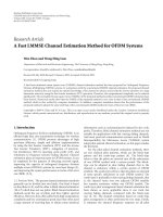
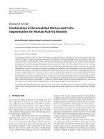
Figure 2: channel impulse response showing sparse structure: (a) is derived from the measured impulse response shown in (b) via the
technique of the appendix.
4. SIMULATIONS
Simulations were carried out to investigate the performance
of the following channel e stimators when different input sig-
nals with different correlation levels are applied.
(A) Standard NLMS channel estimator.
(B) Active-parameter detection-guided NLMS channel es-
timator (as presented in Section 3.2).
(C) APA channel estimator with N
= 10.
(D) FAP channel estimator with N

= 10.
(E) Active-parameter detection-guided FAP channel esti-
mator with N
= 10 (without threshold scaling).
(F) Active-parameter detection-guided FAP channel esti-
mator with N
= 10, with threshold scaling constant.
(G) FAP channel estimator with N
= 14. In this case, it has
almost the same computational complexity
1
as that
of the active-parameter detection-guided FAP channel
estimator with N
= 10.
Simulation conditions are the following.
(a) The channel impulse response considered, as given in
Figure 2(a), was based on a real acoustic echo chan-
nel measurement made by CSIRO Radiophysics, Syd-
ney, Australia. The impulse response of Figure 2(a)
was derived from a measured acoustic echo path im-
pulse response, Figure 2(b), by applying the technique
based on the Dohono thresholding principle [14], as
presented in the appendix. This technique essentially
removes the effects of estimation/measurement noise.
The measured impulse response of Figure 2(b) was ob-
1
The complexity is calculated based on the discussion in Section 3.4.The
computational complexity of the active-parameter detection-guided FAP
channel estimator with N

= 10 is 1980 MPSI, which is slightly lower than
the complexity of standard FAP with N
= 14 of 2044 MPSI.
tained from a room approximately 5 m × 10 m × 3m.
The noise thresholded impulse response of Figure 2(a)
consists of m
= 11 active taps and a total tap length of
n
= 300.
The channel response used in the simulations is an ex-
ample of a room acoustic impulse response which dis-
plays a sparse-like structure. Note, whether or not a
room acoustic impulse response is sparse-like depends
on the room configuration (size, placement of fur-
niture, wall/floor coverings, microphone and speaker
positioning). Nevertheless, a significant proportion of
room acoustic impulse responses are, to varying de-
grees, sparse-like.
(b) Adaptive step size μ
= 0.005.
(c) Regularization parameter δ
= 0.1
(d) Initial channel estimate

θ(0) is the all-zero vector.
(e) Noise signal v(k)
= zero mean Gaussian process with
variance of either 0.01 (Simulations 1 to 3)or0.05
(Simulation 4).
(f) The squared channel estimator error

θ −

θ
2
is plot-
ted to compare the convergence rate. All plots are the
average of 10 similar simulations.
(g) For the simulations of the detection-guided NLMS
channel estimator and the detection-guided FAP chan-
nel estimator, the forgetting parameter γ
= 0.001.
Simulation 1. Lowly correlated coloured input signal u(k)
described by the model u(k)
= w(k)/[1−0.1z
−1
], where w(k)
is a discrete white Gaussian process with zero mean and unit
variance.
Simulation 2. Highly correlated input signal u(k)described
by the model u(k)
= w(k)/[1 − 0.9z
−1
], where w(k)isa
discrete white Gaussian process with zero mean and unit
variance.
Yan Wu Jennifer et al. 7
Simulation 3. Tenth-order AR-modelled speech input signal.
Simulation 4. Tenth-order AR-modelled speech input signal
under noisy conditions. That is, with higher noise variance
= 0.05.

In all four simulations, two detection-guided scaling con-
stants were employed: η
= 1 (i.e., no scaling) and η = 4.
5. RESULT AND ANALYSIS
Simulation 1 (lowly correlated input signal case). The results
of the simulations for channel estimators (a) to (g) with μ
=
0.005 are shown in Figure 3.
(a) Channel estimators (b) to (f) show faster convergence
than the standard NLMS channel estimator (a).
(b) The detection-guided NLMS estimator (b) provides
faster convergence rate than the APA channel estima-
tor (c) with N
= 10 and the FAP channel estimator (d)
with N
= 10. It is clear that the APA channel estimator
(c) with N
= 10 and FAP channel estimator (d) with
N
= 10 still have not reached steady state at the 20000
sample mark.
(c) The detection-guided FAP channel estimators with
N
= 10 (e), (f) show a better convergence rate than
channel estimators (b), (c), and (d).
(d) Detection-guided FAP estimator (e) and detection-
guided FAP estimator with threshold scaling constant
η
= 4 (f) both can detect all the active taps and almost
have the same performance.

(e) With almost the same computational cost, detection-
guided FAP estimator (e) significantly outperforms
standard FAP estimator with N
= 14 in terms of con-
vergence rate.
Simulation 2 (highly correlated input signal case). The re-
sults of the simulations for channel estimators (a) to (g) with
μ
= 0.005 are shown in Figure 4.
(a) The ac tive-parameter detection-guided NLMS chan-
nel estimator (b) does not provide suitably enhanced
improved convergence speed over the standard NLMS
channel estimator (a). This is due to the incorrect de-
tection of many of the inactive taps with the highly cor-
related input signals.
(b) The APA channel estimator with N
= 10 (c) and
the FAP channel estimator with N
= 10 (d) show
significantly improved convergence over (a) and (b).
This is due to the autocorrelation matrix inverse
[U(k)
T
U(k)+δI]
−1
in (5) essentially prewhitening the
highly colored input signal.
(c) The detection-guided FAP channel estimators with
N
= 10 (e), (f) show better convergence rates than the

standard APA channel estimator with N
= 10 (c) and
the standard FAP channel estimator with N
= 10 (d).
In addition, the detection-guided FAP estimators (e),
(f) appear to provide better steady-state error perfor-
mance.
(d) The detection-guided FAP channel estimator (e) with-
out threshold scaling detects extra “nonactive” taps. In
the simulation, it detects 32 active taps, which are 21 in
excess of the true number. This leads to slower conver-
gence rate. In comparison, the detection-guided FAP
channel estimator (f) with threshold scaling η
= 4, it
shows the ability to detect the correct number of active
taps, however, this comes with a relative initial error
increase.
(e) The detection-guided FAP channel estimator (e) with
N
= 10 provides noticeably better convergence rate
performance than the standard FAP channel e stimator
(d) with N
= 14 in terms of the convergence rate and
the steady-state error.
Simulation 3 (highly correlated speech input signal case).
The results of the simulations for channel estimators (a) to
(g) with μ
= 0.005 are shown in Figure 5. The trends shown
here are similar to those of Simulations 1 and 2, although
here the convergence rate and steady-state benefits provided

by detection guiding are further accentuated.
(a) When the speech input signal is applied, the active
parameter detection-guided NLMS channel estimator
(b) suffers from very slow convergence, similar to that
of the standard NLMS channel estimator (a). This is
due to the incorrect detection of many of the inactive
taps.
(b) The detection-guided FAP channel estimators (e) and
(f) significantly outperform channel estimators (c)
and (d) in terms of convergence speed. The results
also indicate that the newly proposed detection-guided
FAP estimators may have better steady state error per-
formance than the standard APA and FAP estimators.
(c) For detection FAP estimator (e) and detection FAP
estimator with threshold scaling constant η
= 4(f),
the trends are similar to those observed for Simula-
tion 2: detection FAP estimator (e) detects extra 23
active taps, resulting in reduced convergence rate and
there is an initial error increase occurring in detection
FAP estimator with threshold scaling constant η
= 4
(f).
(d) Again, with the same computational cost, the detec-
tion-guided FAP channel estimator (e) with N
= 10
shows a faster convergence rate and reduced steady
state error relative to standard FAP channel estimator
(d) with N
= 14.

Simulation 4 (highly correlated speech input signal case with
higher noise variance). The results of the simulations for
channel estimators (a) to (g) with μ
= 0.005 are shown in
Figure 6, which confirm the similar good performance of our
newly proposed channel estimator under noisy conditions.
The detection FAP estimator with threshold scaling constant
η
= 4 (f) performs noticeably better than the detection esti-
mator FAP without threshold scaling (e) due to the ability to
detect the correct number of active taps.
8 EURASIP Journal on Audio, Speech, and Music Processing
10
1
10
0
10
−1
10
−2
10
−3
10
−4
Channel estimation error
00.20.40.60.811.21.41.61.82
×10
4
Sample time
(a)

10
1
10
0
10
−1
10
−2
10
−3
10
−4
Channel estimation error
00.20.40.60.811.21.41.61.82
×10
4
Sample time
(b)
10
1
10
0
10
−1
10
−2
10
−3
10
−4

Channel estimation error
00.20.40.60.811.21.41.61.82
×10
4
Sample time
(c)
10
1
10
0
10
−1
10
−2
10
−3
10
−4
Channel estimation error
00.20.40.60.811.21.41.61.82
×10
4
Sample time
(d)
10
1
10
0
10
−1

10
−2
10
−3
10
−4
Channel estimation error
00.20.40.60.811.21.41.61.82
×10
4
Sample time
(e)
10
1
10
0
10
−1
10
−2
10
−3
10
−4
Channel estimation error
00.20.40.60.811.21.41.61.82
×10
4
Sample time
(f)

10
1
10
0
10
−1
10
−2
10
−3
10
−4
Channel estimation error
00.20.40.60.811.21.41.61.82
×10
4
Sample time
(g)
Figure 3: Comparison of convergence rates for lowly correlated input signal.
Yan Wu Jennifer et al. 9
10
1
10
0
10
−1
10
−2
10
−3

10
−4
Channel estimation error
00.20.40.60.811.21.41.61.82
×10
4
Sample time
(a)
10
1
10
0
10
−1
10
−2
10
−3
10
−4
Channel estimation error
00.20.40.60.811.21.41.61.82
×10
4
Sample time
(b)
10
1
10
0

10
−1
10
−2
10
−3
10
−4
Channel estimation error
00.20.40.60.811.21.41.61.82
×10
4
Sample time
(c)
10
1
10
0
10
−1
10
−2
10
−3
10
−4
Channel estimation error
00.20.40.60.811.21.41.61.82
×10
4

Sample time
(d)
10
1
10
0
10
−1
10
−2
10
−3
10
−4
Channel estimation error
00.20.40.60.811.21.41.61.82
×10
4
Sample time
(e)
10
1
10
0
10
−1
10
−2
10
−3

10
−4
Channel estimation error
00.20.40.60.811.21.41.61.82
×10
4
Sample time
(f)
10
1
10
0
10
−1
10
−2
10
−3
10
−4
Channel estimation error
00.20.40.60.811.21.41.61.82
×10
4
Sample time
(g)
Figure 4: Comparison of convergence rates for highly correlated input signal.
10 EURASIP Journal on Audio, Speech, and Music Processing
10
1

10
0
10
−1
10
−2
10
−3
10
−4
Channel estimation error
00.20.40.60.811.21.41.61.82
×10
4
Sample time
(a)
10
1
10
0
10
−1
10
−2
10
−3
10
−4
Channel estimation error
00.20.40.60.811.21.41.61.82

×10
4
Sample time
(b)
10
1
10
0
10
−1
10
−2
10
−3
10
−4
Channel estimation error
00.20.40.60.811.21.41.61.82
×10
4
Sample time
(c)
10
1
10
0
10
−1
10
−2

10
−3
10
−4
Channel estimation error
00.20.40.60.811.21.41.61.82
×10
4
Sample time
(d)
10
1
10
0
10
−1
10
−2
10
−3
10
−4
Channel estimation error
00.20.40.60.811.21.41.61.82
×10
4
Sample time
(e)
10
1

10
0
10
−1
10
−2
10
−3
10
−4
Channel estimation error
00.20.40.60.811.21.41.61.82
×10
4
Sample time
(f)
10
1
10
0
10
−1
10
−2
10
−3
10
−4
Channel estimation error
00.20.40.60.811.21.41.61.82

×10
4
Sample time
(g)
Figure 5: Comparison of convergence rates for speech input signal.
Yan Wu Jennifer et al. 11
10
1
10
0
10
−1
10
−2
10
−3
10
−4
Channel estimation error
00.20.40.60.811.21.41.61.82
×10
4
Sample time
(a)
10
1
10
0
10
−1

10
−2
10
−3
10
−4
Channel estimation error
00.20.40.60.811.21.41.61.82
×10
4
Sample time
(b)
10
1
10
0
10
−1
10
−2
10
−3
10
−4
Channel estimation error
00.20.40.60.811.21.41.61.82
×10
4
Sample time
(c)

10
1
10
0
10
−1
10
−2
10
−3
10
−4
Channel estimation error
00.20.40.60.811.21.41.61.82
×10
4
Sample time
(d)
10
1
10
0
10
−1
10
−2
10
−3
10
−4

Channel estimation error
00.20.40.60.811.21.41.61.82
×10
4
Sample time
(e)
10
1
10
0
10
−1
10
−2
10
−3
10
−4
Channel estimation error
00.20.40.60.811.21.41.61.82
×10
4
Sample time
(f)
10
1
10
0
10
−1

10
−2
10
−3
10
−4
Channel estimation error
00.20.40.60.811.21.41.61.82
×10
4
Sample time
(g)
Figure 6: Comparison of convergence rates for speech input signal under noisy conditions.
12 EURASIP Journal on Audio, Speech, and Music Processing
6. CONCLUSION
For many adaptive estimation applications, such as acous-
tic echo cancellation within teleconferencing systems, the in-
put signal is speech or highly correlated. In such applications,
the standard NLMS channel estimator suffers from extremely
slow convergence. To remove this weakness, the affine pro-
jection algorithm (APA) or the related computationally ef-
ficient fast affine projection (FAP) algorithm is commonly
employed instead of the NLMS algorithm. Due to the signal
propagation channels in such applications, sometimes hav-
ing low dimensional or sparsely active impulse responses,
we considered the incorporation of active-parameter de-
tection with the FAP channel estimator. This newly pro-
posed detection-guided FAP channel estimator is character-
ized with improved convergence speed and perhaps also bet-
ter steady-state error performance as compared to the stan-

dard FAP estimator. The similar good performance is also
achieved under noisy conditions. Additionally, simulations
confirm these advantages of the proposed channel estima-
tor under essentially the same computational cost. These fea-
tures make this newly proposed channel estimator a good
candidate for the adaptive estimation speech applications
such as the acoustic echo cancellation problem.
APPENDICES
A. SPARSE CHANNEL IMPULSE RESPONSE
ESTIMATION: REMOVING MEASUREMENT
NOISE EFFECTS
In this appendix, a procedure for removing the measure-
ments noise effect from the estimated time domain channel
impulse response is presented. This procedure may be viewed
as an offline scheme for active-tap detection of sparse chan-
nels and assumes that the true impulse response has a suffi-
ciently large number of zero taps. Its applicability is restricted
to channels which have a sparse structure.
In general, the presence of measurement noise or distur-
bance causes the tap coefficient estimate of each of the zero
taps of the sparse channel to be nonzero. If we assume the es-
timate was obtained with a white input, then the discussion
of Section 3 (more details can be found in [ 15]) suggests that
asymptotically (at least for LS, LMS estimates) the zero-tap
estimates have a zero mean i.i.d Gaussian distribution:


θ
i


∼ N

0, σ
2

, i.i.d, where θ
i
= 0. (A.1)
Under the validity of (A.1), we use the following results from
the work of Donoho cited in [15], to develop a procedure for
removing the effects of the noise, or, equivalently, for deter-
mining which taps are zero.
B. RESULT
Let
{

θ
i
} ∼ N(0,σ
2
), i.i.d. Define the eve nt A
M
={sup
i≤M
|z
i
|
≤
σ


2logM}, Then ,Prob(A
M
) → 1asM →∞.
A priori knowledge of the indices i of the zero taps is re-
quired in order to use the threshold σ

2logM to determine
which taps are zero. By applying the foll owing iterative pro-
cedure, this requirement is avoided for sparse channels.
Algorithm 1. (1) Initially, include the indices of all n tap esti-
mates
{

θ
i
} in the set S of zero taps and set M = n.
(2) Determine rms value σ
S
of the estimates of the taps in
Set S.
(3) Determine the indices i of those taps for which the
estimates coefficients satisfy



θ
i


≤

σ
S

2logM. (B.1)
(4) Repeat steps (2) and (3) a g iven number of times or, alter-
natively, until the difference in σ
S
from one iteration to the
next has decreased to a given value.
ACKNOWLEDGMENT
The authors would like to acknowledge CSIRO Rdiophysics,
Sydney for providing the measurement data of the simula-
tion channel.
REFERENCES
[1] K. Ozeki and T. Umeda, “An adaptive filtering algorithm using
an orthogonal projection to an affine subspace and its prop-
erties,” Electronics & Communications in Japan,vol.67,no.5,
pp. 19–27, 1984.
[2]S.L.GayandS.Tavathia,“Thefastaffine projection algo-
rithm,” in Proceedings of the 20th International Conference on
Acoustics, Speech, and Signal Processing (ICASSP ’95), vol. 5,
pp. 3023–3026, Detroit, Mich, USA, May 1995.
[3] J. R. Casar-Corredera and J. Alcazar-Fernandez, “An acous-
tic echo canceller for teleconference systems,” in Proceedings of
IEEE International Conference on Acoustics, Speech and Signal
Processing (ICASSP ’86), vol. 11, pp. 1317–1320, Tokyo, Japan,
April 1986.
[4] A. Gilloire and J. Zurcher, “Achieving the control of the acous-
tic echo in audio terminals,” in Proceedings of European Signal
Processing Conference (EUSIPCO ’88), pp. 491–494, Grenoble,

France, September 1988.
[5] S. Makino and S. Shimada, “Echo control in telecommuni-
caitons,” Journal of the Acoustic Society of Japan,vol.11,no.6,
pp. 309–316, 1990.
[6] J. Homer, I. Mareels, R. R. Bitmead, B. Wahlberg, and A.
Gustafsson, “LMS estimation via structural detection,” IEEE
Transactions on Signal Processing, vol. 46, no. 10, pp. 2651–
2663, 1998.
[7] J. Homer, “Detection guided NLMS estimation of sparsely
parametrized channels,” IEEE Transactions on Circuits and Sys-
tems II, vol. 47, no. 12, pp. 1437–1442, 2000.
[8] J. Homer, I. Mareels, and C. Hoang, “Enhanced detection-
guided NLMS estimation of sparse FIR-modeled signal chan-
nels,” IEEE Transactions on Circuits and Systems I, vol. 53, no. 8,
pp. 1783–1791, 2006.
[9] S. Haykin, Adaptive Filter Theory, Prentice Hall Information
and System Science Series, Prentice-Hall, Upper Saddle River,
NJ, USA, 3rd edition, 1996.
[10] M. Bouchard, “Multichannel affine and fast affine projection
algorithms for active noise control and acoustic equalization
systems,” IEEE Transactions on Speech and Audio Processing,
vol. 11, no. 1, pp. 54–60, 2003.
Yan Wu Jennifer et al. 13
[11] S. G. Sankaran and A. A. Beex, “Convergence behavior of
affine projection algorithms,” IEEE Transactions on Signal Pro-
cessing, vol. 48, no. 4, pp. 1086–1096, 2000.
[12] G. Rombouts and M. Moonen, “A sparse block exact affine
projection algorithm,” IEEE Transactions on Speech and Audio
Processing, vol. 10, no. 2, pp. 100–108, 2002.
[13] G. Rombouts and M. Moonen, “A fast exact frequency do-

main implementation of the exponentially windowed affine
projection algorithm,” in Proceedings of IEEE Adaptive Systems
for Signal Processing, Communications, and Control Symposium
(AS-SPCC ’00), pp. 342–346, Lake Louise, Alta., Canada, Oc-
tober 2000.
[14] M. R. Leadbetter, G. Lindgren, and H. Rootzen, Extremes and
Related Properties of Random Sequences and Processes, Springer ,
New York, NY, USA, 1982.
[15] H. Cramer and M. R. Leadbetter, Stationary and Related
Stochastic Srocesses: Sample Function Properties and Their Ap-
plications, John Wiley & Sons, New York, NY, USA, 1967.