Báo cáo hóa học: " Research Article Linear Predictive Detection for Power Line Communications Impaired by Colored Noise" pdf

Hindawi Publishing Corporation
EURASIP Journal on Advances in Signal Processing
Volume 2007, Article ID 32818, 12 pages
doi:10.1155/2007/32818

Research Article
Linear Predictive Detection for Power Line Communications
Impaired by Colored Noise
Riccardo Pighi and Riccardo Raheli
Dipartimento di Ingegneria dell’Informazione, Universit` di Parma, Viale G. P. Usberti 181A, 43100 Parma, Italy
a
Received 10 November 2006; Revised 21 March 2007; Accepted 13 May 2007
Recommended by Lutz Lampe
Robust detection algorithms capable of mitigating the effects of colored noise are of primary interest in communication systems
operating on power line channels. In this paper, we present a sequence detection scheme based on linear prediction to be applied
in single-carrier power line communications impaired by colored noise. The presence of colored noise and the need for statistical
sufficiency requires the design of an optimal front-end stage, whereas the need for a low-complexity solution suggests a more practical suboptimal front-end. The performance of receivers employing both optimal and suboptimal front-ends has been assessed by
means of minimum mean square prediction error (MMSPE) analysis and bit-error rate (BER) simulations. We show that the proposed optimal solution improves the BER performance with respect to conventional systems and makes the receiver more robust
against colored noise. As case studies, we investigate the performance of the proposed receivers in a low-voltage (LV) power line
channel limited by colored background noise and in a high-voltage (HV) power line channel limited by corona noise.
Copyright © 2007 R. Pighi and R. Raheli. This is an open access article distributed under the Creative Commons Attribution
License, which permits unrestricted use, distribution, and reproduction in any medium, provided the original work is properly
cited.

1.

INTRODUCTION

In the last years, there has been a growing interest towards
the possibility of exploiting existing power lines as effective
transmission means [1, 2]. Low-voltage (LV) and mediumvoltage (MV) power lines, below 1 kV and from 1 to 36 kV,

respectively, are appealing because they provide a potentially convenient and inexpensive communication medium
for control signaling and data communication. The structure
of the distribution grid is also appropriate for internet access
[3], and the existing lines can be used as backbone for local
area networks or wide area networks, as a solution to the “last
mile” access problem [4]. Even though power lines are an attractive solution for data transmission, a reliable high-speed
communication is a great challenge due to the nature of the
medium.
Communication systems over power lines have to deal
with a very harsh environment [2]. Since the power grid
was originally designed for electrical energy delivery rather
than for data transmission, the power line medium has several less than ideal properties as a communication channel
and, as a consequence, calls for communication techniques
able to cope effectively with this hostile environment. The
transmission medium of the power grid is characterized by

a time-varying attenuation [5] and frequency selectivity [6],
with possibly deep spectral notches, depending also on the
location. Any transmission scheme applied to power lines
has to cope with these impairments, including the intrinsic dependence of the channel model on the network topology and connected loads, the presence of high-level interference signals due to noisy loads, and the presence of colored noise. Moreover, the channel conditions can change because of connections and disconnections of inductive or capacitive loads. Finally, reflections from impedance mismatch
at points where equipments are connected or from nonterminated points can result in multipath [7–9] and various
types of noise [10].
High-voltage (HV) power lines, typically operating at or
above 64 kV, can also be used for communication purposes,
for example, in scenarios not covered by wireless or wired
telecommunication infrastructures.
In low- or medium-voltage power grids, several noise
sources can be found, such as, for example [11], (i) nonstationary colored thermal noise with power spectral density decreasing as the frequency increases, (ii) periodic asynchronous impulse noise related to switching operations of
power supplies, (iii) periodic synchronous impulse noise
mainly caused by switching actions of rectifier diodes, and

2

EURASIP Journal on Advances in Signal Processing

(iv) asynchronous impulse noise [12]. On the other hand,
the HV power line channel is also limited by disturbances
produced by events outside the transmission channel such
as, for example, atmospheric phenomena, lightning [13], or
disturbances originating within the system such as network
switching [10], impulse noise [14–17], and corona phenomena [18–20].
In power line communications, single-carrier modulations based on quadrature amplitude modulation (QAM) or
other modulation formats may be adopted for their simplicity. However, in broadband applications strong colored noise
sources can severely limit the performance of single-carrier
systems and demand for adequate signal processing schemes.
In this paper, we propose a single-carrier PLC scheme
based on linear prediction and multidimensional coding,
which exhibits good improvements, in terms of signal-tonoise ratio (SNR) necessary to achieve a given bit-error rate
(BER), with respect to state-of-the-art solutions. The principle of linear predictive detectors proposed for fading channels [21–24] is a valuable and general technique that can be
used every time a communication system has to cope with
colored noise [25], provided that a correct statistical information on the noise is available at the receiver. First, we will
introduce the linear predictive detection scheme considering
a general model for the colored noise process. As case studies,
we will also analyze the performance of the proposed receiver
considering colored background noise for LV power lines and
corona noise [19, 20] for HV power lines.
Moreover, in order to reduce the computational load
of the linear predictive receiver, we apply reduced-state sequence detection techniques [26–29] such as “trellis folding by set partitioning” [30] and per-survivor processing
(PSP) [29], and demonstrate the robustness of the proposed

scheme in terms of BER and complexity with respect to standard solutions.
This paper expands upon preliminary work reported in
[31]. With respect to [31], this paper complements the analysis comparing the BER performance of the optimal and suboptimal solutions in the presence of frequency selective LV
and HV power line channels. In particular, main contributions of the article are the following:
(1) to demonstrate and compare the performance, in
terms of SNR, of suboptimal and optimal front ends;
(2) for a given front end, to quantify the SNR improvements achievable by the linear predictive approach;
(3) to address the complexity of the proposed solution
by means of state reduction techniques such as trellis
folding by set partitioning and per-survivor processing;
(4) to extend the linear prediction algorithm to a multidimensional TCM code;
(5) to demonstrate that the linear predictive detection is
an advanced signal processing technique which may
be effectively applied to power line communications
in order to increase the system robustness to colored
noise.
The paper outline is as follows. In Section 2, we present
the reduced-state multidimensional linear prediction re-

ceiver based on an optimal front end or a suboptimal practical approximation. In Section 3, we describe how linear prediction can be applied to a multidimensional observable. In
Sections 4 and 5, we introduce, respectively, the channel and
the colored noise models for an LV and HV power line scenarios. In Section 6, numerical results are presented. Finally,
Section 7 concludes the paper.
2.

LINEAR PREDICTION RECEIVER

Single-carrier transmission may be attractive from a complexity point of view. However, since the power line channel
is affected by severe intersymbol interference (ISI) and colored noise, powerful detection and equalization techniques
are necessary. Practical implementation of these schemes

may also require reduced state approaches.
2.1.

Optimal detector

Let us consider the transmission scheme depicted in Figure 1
in terms of its lowpass equivalent. We adopt a transmission
system based on a four-dimensional trellis coded modulation scheme (4D-TCM) [32], which is a suitable choice to
achieve high spectral efficiency and, at the same time, a good
coding gain. We assume a square-root raised cosine shaping
filter with frequency response P( f ) and a power line channel with frequency response H( f ), which will be detailed in
Sections 4 and 5. The presence of colored noise η(t) with
power spectral density (PSD) given by Sη ( f ), and the need
for statistical sufficiency yield a detector front end based on a
whitening filter, with frequency response 1/ Sη ( f ), and a filter matched to the overall channel response Q∗ ( f )/ Sη ( f ),
where Q( f ) = P( f )H( f ), namely, a standard matched filter
for colored noise [33]. The signal at the output of this filter is sampled with period equal to the signaling interval T.
The frequency selectivity of the power line channel may be
dealt with by an equalizer which limits the ISI. This equalizer can be used to reduce the amount of ISI and, as a consequence, the trellis complexity of the following sequence detector based on a Viterbi processor. As extreme cases, the
equalizer may be omitted, relegating the task of dealing with
ISI to the detector, or it can be very complex in order to substantially eliminate the ISI. The following derivation is general enough to encompass, as special cases, these extreme scenarios, as well as intermediate ones. After the equalizer, we
use a sequence detection Viterbi processor to search an extended trellis diagram accounting for the encoder memory,
the residual ISI and the channel memory induced by colored
noise. This detector uses linear prediction to deal with the
colored noise at its input.
As a consequence, considering the system model in
Figure 1, the discrete-time observable at the input of the
Viterbi processor can be expressed as
L

ri =

fn ci−n +ni ,
n=0
si (cii−L )

(1)


R. Pighi and R. Raheli

{ak }

3

4D-TCM
encoder

ck

P( f )

H( f )

PLC channel

1
Sη ( f )

+

Q∗ ( f )

t = iT
EQ

Sη ( f )

ri

Viterbi
proc.

{ak }

η(t)
Whitening & matched filter

Figure 1: Simplified system model with optimum receiver for colored noise.

where1 fi = gi ⊗ di denotes the overall impulse response of
the system, gi = g(t)|t=iT = p(t) ⊗ h(t) ⊗ m(−t)|t=iT is the impulse response up to the output of the sampling device with
p(t) = F −1 {P( f )}, F −1 being the inverse Fourier transform operator, h(t) = F −1 {H( f )}, m(t) = F −1 {M( f )} and
M( f ) = Q∗ ( f )/S( f ), di is the impulse response of the equalizer, si (cii−L ) is the noiseless signal component affected by the
residual ISI of length L at the output of the equalizer, {ci } is
the code sequence with symbols belonging to a QAM constellation, and {ni } is a sequence of colored noise samples
with PSD Sn (ej2π f T ). Note that the noise at the output of the
matched filter Q∗ ( f )/ Sη ( f ) is colored with a different PSD
with respect to that associated to η(t). Moreover, the presence
of the equalizer changes also the spectral density of the noise

at the input of the Viterbi processor. Finally, we assume that
the colored noise can be modeled as a process with Gaussian
statistics.
We now derive the optimal branch metric for a singlecarrier communication scheme to be used in a sequence detection Viterbi algorithm. Collecting the samples (1) at the
output of the colored noise channel into a suitable complex
vector r, we can formulate the maximum a posteriori probability (MAP) sequence detection strategy as
a = arg max p(r | a)P {a},
a

(2)

where p(r | a) is the conditional probability density function (PDF) of the vector r, given the data vector a, and P {a}
is the a priori probability of the information symbols. Since
the trellis encoder can be described as a time-invariant finite
state machine, it is possible to define a sequence of 4D states
{μ0 , μ1 , . . . } over which the encoder evolves and define a deterministic state transition law, function of the 4D information symbol ak , which describes the evolution of the system,
that is, μk = f (μk−1 , ak−1 ). Note that each state μk belongs
to a set of finite cardinality. As a consequence, the evolution
of the finite state machine model of the 4D-TCM encoder
can be described through a trellis diagram, in which there
are a fixed number of exiting branches from each state: this
number will depend on the number of subsets in which the
constellation is partitioned [34].
The 4D-TCM code symbol Ck (ak , μk ) = (c2k−1 (ak , μk ),
c2k (ak , μk )), with 2D components belonging to a QAM constellation, is a function of the encoder state μk and the information symbol ak at the input of the encoder. Note that
1

The operator ⊗ denotes convolution in continuous or discrete time.

c2k−1 (ak , μk ) and c2k (ak , μk ) are, respectively, the first and

second two-dimensional (2D) symbols transmitted over the
channel during the four-dimensional time interval. Under
these assumptions, we can express the 4D discrete-time observable as Rk = (r2k−1 , r2k ), where the 2D components are
defined according to (1).
Assuming causality and finite memory [35], applying the
chain factorization rule to the conditional PDF and taking
into account the multidimensional structure of the TCM
code, we can rewrite (2) as
K −1

a = arg max
a

k=0
K −1

arg max
a

k
k
p Rk | R0−1 , a0 P ak

k=0

p r2k | r2k−1−ν , ak , ζk
2k−2

(3)

· p r2k−1 | r2k−2−ν , ak , ζk P ak ,
2k−2

where K is the length of the transmission and rk2 is a shortk1
hand notation for a vector collecting 2D signal observations
from time epoch k1 to k2 . In the last step of (3), in order to
limit the memory of the receiver, we have assumed Markovianity of order ν in the conditional observation sequence.
Moreover we define a system state accounting for the 4DTCM coder state μk , the order of Markovianity ν, and the
residual ISI span L as
ζk = μk , Ck−1 , Ck−2 , Ck−3 , . . . , Ck−(L+ν)/2
= μk , c2k−1 , c2k−2 , . . . , c2k−ν−L .

(4)

The assumed Markovianity results in an approximation
whose quality increases with the order ν.
Since we assume that the colored noise process has a
Gaussian distribution, the observation is conditionally Gaussian, given the data. The application of the chain factorization rule allows us to factor the conditional PDF in (3) as
a product of two complex conditional Gaussian PDFs, completely defined by the conditional means
r2k = E r2k | r2k−1−ν ; ak , ζk ,
2k−2
r2k−1 = E r2k−1 | r2k−2−ν ; ak , ζk ,
2k−2

(5)

and the conditional variances
σr22k = E r2k − r2k

2

| r2k−1−ν ; ak , ζk ,
2k−2

σr22k−1 = E r2k−1 − r2k−1

2

| r2k−2−ν ; ak , ζk .
2k−2

(6)


4

EURASIP Journal on Advances in Signal Processing

These conditional means r2k and r2k−1 can be interpreted as
perhypothesis linear predictive estimates of r2k and r2k−1 , respectively; likewise, the conditional variances σr22k and σr22k−1
are interpretable as the relevant minimum mean square prediction errors (MMSPEs) [36]. Note that, for a given value
of ν, the number of prediction coefficients changes with respect to the number of past samples defined in the conditioning event, that is, r2k−1 is evaluated using the last ν 2D
observables, whereas r2k is evaluated using the last ν + 1 2D
observables. The solution of a Wiener-Hopf matrix equation
for linear prediction based on a 4D observable will be presented in Section 3.
The detection strategy (2), the factorization (3), and linear prediction allow us to derive the branch metrics to be
used for joint sequence detection and decoding in a Viterbi
algorithm. Taking the logarithm, assuming that the information symbols are independent and identically distributed
and discarding irrelevant terms, we can express the metric of
branch (ak , ζk ) as

The branch metric can be obtained by defining a “pseudo
state” [30]
ζk ωk =

μk , Ck−1 ωk , . . . , Ck−Q ωk ,
Q+1 elements

˘
˘
Ck−Q−1 ωk , . . . , Ck−Q−P ωk

λk ak , ζk ∝

where Ck−1 (ωk ), . . . , Ck−Q (ωk ) are Q code symbols compatible with state ωk to be found in the survivor history of state ωk , and P are code symbols chosen by
a per-survivor processing (PSP) technique [29], that is,
˘
˘
Ck−Q−1 (ωk ), . . . , Ck−Q−P (ωk ) are the P 4D-TCM code symbols associated with the survivor of ωk . The branch metric
λk (Ik (1), ωk ) in the reduced-state trellis can be defined in
terms of the pseudostate (12) according to

i=0

Ck ∈Ik (1)

ln p r2k−i | r2k−1−iν ; ak , ζk ,
2k−2−

(7)

where the symbol ∝ denotes a monotonic relation with respect to the variable of interest (i.e., the data sequence). The
detection strategy (2) can be now formalized as
K −1

a = arg min
a

λk ak , ζk ,

(8)

k=0

where the branch metrics are expressed as
1

λk ak , ζk =
i=0

r2k−i − r2k−i
σr22k−i

2

+ ln σr22k−i .

(9)

Finally, the state complexity of a linear predictive receiver

can be limited by means of state-reduction techniques [26–
29]. Let S = Sc M (ν+L)/2 denote the state complexity of the
proposed receiver, where Sc is the number of states of the 4DTCM encoder, M is the cardinality of the 2D constellation,
and Q < (ν + L)/2 + 1 denotes the memory parameter taken
into account in the definition of a “reduced” trellis state
ωk = μk , Ik−1 (1), Ik−2 (2), . . . , Ik−Q (Q)

(10)

in which, for i = 1, . . . , Q, Ik−i (i) ∈ Ω(i) are subsets of the
code constellation and Ω(i) are partitions of the code constellation.2 Defining Ji = card{Ω(i)}, i = 1, . . . , Q as the cardinality of the partition Ω(i), the number of reduced-states
in the trellis diagram can be expressed as [26, 28]
Q

S = Sc
i=1

2

Ji
.
2

Ck−i ∈ Ω(i) are 4D-coded symbols compatible with the given state.

(11)

,

P code symbols

λk Ik (1), ωk = min λk ak , ζk ωk
1

(12)

(13)

assuming that the pseudo state ζk (ωk ) is compatible with ωk ,
that is, Ck−i ∈ Ik−i (i).
As already noted in Section 2.1, we point out the fact
that the formulation of the reduced-state linear predictive
approach detailed in this article is general and its validity is
independent from the ISI-removing capacity of the equalizer.
In particular, if the equalizer is ideal, L should be set to zero; if
a realistic equalizer is used, some residual ISI may be present
and can be duly accounted for by a proper selection of L.
Finally, if the equalizer is absent, it is still possible to encompass the ISI using a joint sequence detection and decoding
approach. In conclusion, the proposed approach may be applied to every kind of equalization scheme. In the absence of
explicit knowledge of the amount of residual ISI, it is possible to select a sufficiently large value for L. However, since
the parameter L affects the complexity of the Viterbi processor, the selected value should be kept as small as possible in
order to limit the implementation cost.
2.2.

Suboptimal detector

Since the optimal front end may be quite complex from
a practical point of view, requiring adaptivity and highcomputational load during the filtering process, in Figure 2, a
suboptimal, more practical alternative is also presented. Instead of performing the whitening operation in the analog
front-end stage, we propose a linear predictive receiver in

which signal processing, necessary for coping with the colored noise, is entirely done in a digital fashion, that is, modifying the branch metric of a Viterbi processor. The shaping and receiver filter can be both selected with square-root
raised cosine frequency response, so that noise samples are
white when the overall noise process is white. Since the signal processing associated to the suboptimal front end is different from the processing done by the optimal front end, the
PSD of the colored noise at the input of the Viterbi processor is different. Moreover, we still assume that the equalizer


R. Pighi and R. Raheli

5
t = iT

{ak }

4D-TCM
encoder

ck

P( f )

+

H( f )

P∗ ( f )

EQ

ri

Viterbi
proc.

{ak }

η(t)
PLC channel

Figure 2: Simplified system model with a suboptimal implementation of the front-end filter.

may leave some residual ISI into the signal at the input of the
Viterbi processor: under this assumption, the discrete time
observable ri may be defined as in (1), with a different impulse response fi and noise spectrum.
The proposed suboptimal front end may be used to
upgrade a PLC system, originally not designed for a scenario limited by colored noise, by simply modifying the
Viterbi processor while leaving unchanged the, possibly analog, front-end stage. As previously outlined, the Viterbi processor enables sequence detection and decoding, searching
an extended trellis diagram including the residual ISI and the
code memory, using a branch metric defined as in (9) and
possibly state-reduction techniques as presented in (12) and
(13).
Finally, note that the proposed suboptimal solution with
linear prediction may be an effective approach for communication systems which have to deal with time-varying channel conditions, simplifying the adaptivity of the receiver. In
particular, it is possible to recursively adapt the values of the
prediction coefficients by applying standard techniques, like
those based on stochastic gradient algorithms [36].
3.

MULTIDIMENSIONAL LINEAR PREDICTION

In this section, we describe how linear prediction can be applied to a 4D observation vector collecting Rk and how to

obtain an estimate of the colored noise samples at the output of the matched filter. We start defining a cost function J
which represents the conditional mean square error between
the colored noise samples and a possible set of estimates of
the noise process.
It is possible to express the cost function as3
J(P) = E

{Rk−i − Sk−i (Ck−i−L/2 )}ν/2 are related to the data [36], that is,
i
k−i

the per-survivor past samples of colored noise, to be used to
perform linear prediction.
The cost function (14) can be expressed explicitly as

ν/2

−
i=1

p1,i r2k−1−i − s2k−1−i c2k−1−ii−L
2k−1−

r2k − s2k c2k−L
2k

+
ν

−

i=0

2

p2,i r2k−1−i − s2k−1−i c2k−1−ii−L
2k−1−

| ak , ζk ,

i

| ak , ζk .

(15)
Since the cost function is a sum of two positive functions of
disjoint sets of variables, that is, J(P) = J1 (p1 ) + J2 (p2 ) with
p1 and p2 , respectively, the prediction vectors for the first and
second 2D observable, the minimization can be performed
separately on each function. In the following, we show how
to obtain the prediction coefficients for the first 2D component of the 4D observable (i.e., { p1,i }). Defining data vectors
d2k−2−ν = r2k−2−ν − s2k−2−ν c2k−2−ν−L
2k−2
2k−2
2k−2
2k−2

T

(16)

collecting ν per-survivor noise samples at the input of the
Viterbi processor, we can express the cost function as4
J1 p1 = E

d2k−1 − pT · d2k−2−ν
1
2k−2
· d2k−1 − pT · d2k−2−ν
1
2k−2

2

Pi Rk−i − Sk−i Ck−ii−L/2
k−

2

ν

Rk − Sk Ck−L/2
k
−

r2k−1 − s2k−1 c2k−1−L
2k−1

J(P) = E

H

| ak , ζk .

(17)

Taking the gradient with respect to the prediction vector
p1 we are now able to formulate the Wiener-Hopf equation
as

(14)
where P is a matrix collecting all prediction coefficients,
Sk (Ck−L/2 ) is the noiseless 4D signal component affected by
k
ISI and · 2 is the Euclidean norm. The quantity Rk −
Sk (Ck−L/2 ) represents the colored noise sample we wish to
k
predict on the correct trellis path. Similarly, the quantities
3

For notational simplicity, we omit the dependence of the code symbol on
the state ζk and input symbols ak , that is, Ck is used in place of Ck (ak , ζk ).

Rν · p1 = qν ,

(18)

where the system matrix, with dimension ν × ν, is defined as
Rν = E d2k−2−ν · d2k−2−ν
2k−2
2k−2

4

H

| ak , ζk

(19)

Superscripts T and H denote transpose and Hermitian transpose operators, respectively.


6

EURASIP Journal on Advances in Signal Processing

and the vector of ν known terms is
qν = E d2k−1 d2k−2−ν | ak , ζk .
2k−2

(20)

We remark that the per-survivor noise samples d2k−2−ν
2k−2
are not available at the detector: they must be evaluated
through the observation of the output of the front end and
a reconstruction of noiseless signal components associated
with the survivor path leading to state ζk .
The linear system defined in (18) can now be solved using
Cholesky factorization [36], obtaining the prediction coefficient vector

−
p1 = Rν 1 · qν .

(21)

As to the second 2D observable, the prediction coefficients
{ p2,i } and the cost function J2 (p2 ) can be determined in a
similar manner, noting that in the evaluation of the estimate
E{r2k | r2k−1−ν ; ak , ζk } we can also use the observable at time
2k−2
2k − 1 from the most recent previous 2D observable.
Finally, rewriting the cost functions J1 (p1 ) and J2 (p2 ) as
explicit functions of the predictor vectors p1 and p2 , respectively, we can express the minimum mean square prediction
errors as
2
J1 p1 = σn − pT · qν
1
2
J2 p2 = σn − pT · qν+1 ,
2

(22)

2
where σn is the colored noise power at the input of the Viterbi
processor.

4.

4.2.

LV power line channels have a tree-like topology with
branches formed by additional wires connected to the main
path, having different length and different load impedence.
The channel exhibits notches due to reflections caused by
impedence mismatches. Several approaches for modeling the
transfer function of LV power lines can be found in the literature. Probably, the most widely known model for the channel frequency response Hc ( f ) of LV and MV PLC channels is
the multipath model proposed by Philipps [7] and Zimmermann and Dostert [8]. Following this model, the frequency
response of the channel may be expressed, in the frequency
range from 500 kHz to 20 MHz, as6
N

LOW- AND MEDIUM-VOLTAGE
POWER LINE CHANNEL

gi e−(a0 +a1 f

k )d

i

e−j2π f di /v p ,

(24)

i=1

Besides frequency selectivity, the dominant channel disturbances occurring in power line channels in the frequency
range between a few hundred kHz and 20 MHz are colored background noise, narrowband interference and impulse noise. Some measurements at high frequencies have
been reported in [37, 38]. In this work, we represent the colored PSD using a simple three-parameter model presented in

[39], that is,5
Sηc ( f ) = a + b · | f |c

Channel model

Hc ( f ) =

4.1. Colored noise model

dBm
Hz

(23)

with a = −145, b = 53.23 and c = −0.337. Despite the fact
that a realistic PSD may present some variations with respect
to the PSD predicted by (23), this simple model allows us
to capture the main characteristic of the colored background
noise, that is, the fact that the PSD decreases as the frequency
increases.
Note that (23) defines a power spectrum whose frequency components are over the entire frequency domain,
5

that is, its bandwidth is generally greater than that used by the
transmission system. In our simulation, we derive an equivalent complex lowpass filtered version of the colored background noise process within the bandwidth of the considered
signaling scheme. The filter used for the generation of colored noise is a finite impulse response (FIR) complex filter
with coefficients obtained using Cholesky factorization [36]
applied to the complex lowpass filtered colored noise power
spectrum.
Finally, it should be pointed out that the noise in power

lines may be modeled as nonstationary [40]. In this work, we
assume that the changes in the noise PSD are slow enough to
allow a correct estimation of the prediction coefficients.

Note that Sη ( f ) in Figures 1 and 2 is the lowpass equivalent PSD of Sηc ( f )
with respect to the carrier frequency.

where N is the number of relevant propagation paths, a0
and a1 are link attenuation parameters, k is an exponent
with typical values ranging from 0.5 to 1, gi is the weighting factor for path i, di is the length of the ith path, and v p
is the phase velocity. In this work we consider a PLC channel
modeled by (24) with parameters [8] a0 = 0, a1 = 8.10−6 ,
k = 0.5, N = 4, {gi }4=1 = {0.4, −0.4, −0.8, −1.5}, and
i
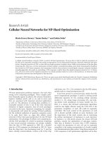
{di }4=1 = {150, 188, 264, 397}. In Figure 3 the LV power line
i
channel amplitude response based on these parameter values
along with an idealized spectrum used by the systems considered in our simulations are shown.
5.
5.1.

HIGH-VOLTAGE POWER LINE CHANNEL
Corona noise model

The PLC channel may consist of one or more conductors, depending on the considered coupling scheme, that is, phase-to
ground or phase to phase [41]. Corona noise is a common
noise source for HV transmission lines, since it is permanent
and its intensity depends on (i) the service voltage, (ii) the
geometric configuration of the power line, (iii) the type of
6

Note that H( f ) in Figures 1 and 2 is the lowpass equivalent of Hc ( f ) with
respect to the carrier frequency.


R. Pighi and R. Raheli

7
Table 1: Values of the digital filter coefficients {v }4=1 in (25) for
various service voltages.

0

Frequency response (dB)

−10

v1

Voltage [kV]
225
380
750
1050

−20
−30
−40

−1.225

−1.298
−1.302
−1.292

v2
1.052
1.109
1.041
1.080

v3
−0.603
−0.625
−0.611
−0.647

v4
0.217
0.210
0.207
0.224

−50
−60

10
Signal spectrum

9

−70
−80

8
2500

5000

7500 10000 12500 15000 17500 20000

7

Figure 3: Frequency response of the simulated LV power line channel and the transmission spectrum used by the considered singlecarrier PLC system.

|V( f )|2

Frequency (kHz)

6
5
4
3
2

conductors involved in the line and (iv) the atmospheric conditions.
Corona noise is caused by partial discharges on insulators and in air surrounding electrical conductors of power
lines [42]. When HV power lines are in operation, the voltage
originates a strong electric field in the vicinity of the conductor. This electric field accelerates free electrons present in the
air nearby conductors: these electrons collide with molecules
of the air, generating a free electron and positive ion couple.

This process continues forming an avalanche phenomenon
called “corona discharge.” The motion of positive and negative charges induces a current both in the conductors and
ground [18].
The induced current appears like a train of current
pulses, with random pulse amplitude variations and random
interarrival intervals. The injected current due to corona
noise on one conductor can be modeled by a current
source [18, 42]: according to Shockley-Ramo theorem [41],
a corona discharge induces current in all conductors, that is,
each conductor of the power line channel is connected to the
ground by a current source.
A few corona noise models are present in the literature
[13, 18–20]: in this article, the model proposed in [19, 20] is
considered. Corona noise, as a random signal, is characterized equivalently through its autocorrelation function or its
power spectrum. To this purpose, the corona noise spectrum
is generated by a method that takes into account the generation phenomena of corona currents injected in the conductors and the propagation along the line [43, 44]. This spectrum is utilized to synthesize an autoregressive (AR) digital
filter [36], whose output is described by the expression

1
0

100

200

300 400

500

600

700

800

900 1000

Frequency (kHz)
225 kV line
380 kV line

750 kV line
1050 kV line

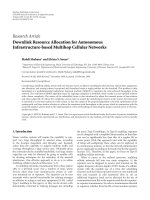
Figure 4: Corona noise power spectrum, shown in terms of the frequency response V ( f ) of the AR filter in (25).

modeling the corona noise process. The synthesis of the digital filter essentially calls for the identification of the coefficients {v }N=1 and can be done using a procedure based on
the maximum entropy method proposed in [45] or on the
minimization of the difference between estimated and measured power spectra.
Table 1 shows, for N = 4, a complete set of coefficients
modeling the corona noise for different voltage lines with
carrier couplings of lateral phase-to-ground type [20].
Note that, as already outlined, (25) defines a corona
power spectrum whose frequency components are over the
entire frequency domain, that is, its bandwidth is generally
greater than that used by the transmission system. As a consequence, we derive an equivalent lowpass-filtered complex
version of the corona noise process within the bandwidth
of the considered signaling scheme. In Figure 4, the corona
noise power spectrum obtained with the model presented in
(25) with coefficients shown in Table 1 is also presented in

terms of the power frequency response |V ( f )|2 of the AR
digital filter.

N

nk =

v nk − + w k ,

(25)

=1

where {wk } is a sequence of independent zero-mean Gaussian random variables and {v }N=1 is the set of coefficients

5.2.

Channel model

In this section, we describe the model used for an HV power
line channel. Since the transfer function of HV power lines


8

EURASIP Journal on Advances in Signal Processing
0

−1.2

−10

−1.6
−2
−2.4

−30

MMSPE (dB)

Frequency response (dB)

−20

−40
−50
−60
−70

−3.2
−3.6
−4
−4.4

Optimal front end

−5.2

Signal spectrum

−5.6

−90

−6

0

50

100

150

200

250

300

350

400 450

0

500

Figure 5: Frequency response of the considered 225 kV power line
channel and the transmission spectrum used by the single-carrier

PLC system.

exhibits a strong dependence on the operating atmospheric
conditions and on the different kind of loads connected to
the line, a universally accepted model for the impulse response of the channel has still not been formulated. As a consequence, in this work we have used a simple HV channel
model as similar as possible to a realistic scenario, including the most important limiting characteristics, that is, frequency selectivity and high attenuation.
Figure 5 shows the transfer function Hc ( f ) used in our
simulation to model a 225 kV channel along with an idealized spectrum used by the systems considered in our simulations. Note that, due to the lowpass frequency response of the
coupling devices and regulatory standards, the transmission
bandwidth for HV power line communications is limited to
a range from 100 to 500 kHz.
NUMERICAL RESULTS

In this section, we provide the numerical results obtained applying the proposed reduced-state linear predictive solutions
to two different scenarios. First, we compare the performance
of a single-carrier transmission system operating on an LV
power line channel affected by colored background noise using the optimal and suboptimal front ends. Then we consider the performance of a single-carrier transmission system
working on an HV power line channel impaired by corona
noise, using either the optimal or the suboptimal front end.
The SNR is defined at the input of the receiver as Eb /N0 ,
where Eb is the received energy per information bit and N0 is
defined as the average equivalent white noise intensity which
yields the total noise power in the transmission bandwidth B
at the input of the receiver
N0 =

1
B

B

Sη ( f )df .

1

2

3

4

5

6

7

8

9

10

Prediction order ν

Frequency (kHz)

6.

Eb /N0 = 20 dB

64 QAM
Background noise

Suboptimal front end

−4.8

−80

−100

−2.8

(26)

Cost function J1 (p1 )
Cost function J2 (p2 )

Figure 6: MMSPEs, normalized to the power of the signal si (cii−L ),
as a function of the prediction order ν, assuming a 64 QAM constellation, signaling frequency fs = 2.4 MHz, and carrier frequency
fc = 6 MHz.

Since the main focus of this paper is on linear predictive detection for colored noise, we assume that the equalizer
shown in Figures 1 and 2 is an ideal zero-forcing equalizer
able to completely remove the ISI introduced by the channel
(L = 0). As a consequence, the discrete-time signal at the input of the Viterbi processor can be modeled according to (1)
with L = 0.
Finally, note that the stationarity assumption for the
channel and noise is acceptable for LV PLC because the signaling frequency fs is much larger than the main frequency.
As to HV PLC, the main source of colored noise, that is, the

corona noise, presents a quasistationary nature with a rate
of change that is orders of magnitude lower than the signaling frequency fs , that is, its variation is very slow compared
with the signaling period used by the PLC system. As a consequence, the assumption of stationarity for the corona noise
is also very reasonable.
6.1.

Low-voltage channel: MMSPE analysis

Let us consider first a single-carrier PLC system operating
on an LV power line with frequency response defined as in
Section 4.2. We adopt a transmission system based on an 8state 4D-TCM code applied to a 64 QAM constellation, a
square root raised cosine pulse as shaping filter with a rolloff factor α equal to 0.3, a signaling and carrier frequencies
equal to, respectively, fs = 2.4 MHz and fc = 6 MHz.
In Figure 6, the performance of the linear predictor is assessed in terms of MMSPEs versus the prediction order ν for
a fixed Eb /N0 of 20 dB. In this figure the MMSPE has been
normalized to the power of the useful signal si (cii−L ). The colored background noise process is generated according to the
model presented in Section 4.1. We show the cost function


R. Pighi and R. Raheli

9
−4.2

100

−4.4

Suboptimal front end

10−1

−4.6

MMSPE (dB)

Bit error rate

−4.8

Optimal front end

10−2
10−3
10−4

Suboptimal front end

−5
−5.2
−5.4

Eb /N0 = 20 dB
16 QAM
Corona noise

−5.6
−5.8

Optimal front end

−6
−6.2

10−5

−6.4

10−6

2

4

6

8

10

12 14 16
Eb /N0 (dB)

18

20

22

−6.6

24

Optimal front end, ν = 0
Optimal front end, ν = 2
Optimal front end, ν = 8
Suboptimal front end, ν = 0
Suboptimal front end, ν = 2
Suboptimal front end, ν = 8

Figure 7: Performance of the proposed receivers for 4D-TCM 64
QAM and various values of prediction order, obtained with an 8state 4D-TCM code applied to a 64 QAM constellation, signaling
frequency fs = 2.4 MHz and carrier frequency fc = 6 MHz. The LV
power line channel is modeled as in Section 4.2.

J1 (p1 ) related to the estimate of the first 2D observable and
the cost function J2 (p2 ) related to the second 2D observable.
Note that the prediction order ν is expressed in terms of signaling intervals, that is, ν = 2 means that two 2D observables are needed for the computation of r2k−1 and three 2D
observables are used for the computation of r2k . The continuous lines in Figure 6 show the normalized MMSPE performance achievable using the optimal front end, while the
dashed lines present the MMSPE gain obtained using the
suboptimal front end. Assuming a prediction order ν = 8,
the MMSPE gain shown in Figure 6 is 1.8 dB for the optimal
receiver and 2.4 dB for the suboptimal receiver.
6.2. Low-voltage channel: BER analysis
Continuous lines (curves with labels “optimal front end”)
and dashed line (curves with labels “suboptimal front end”)
in Figure 7 show, respectively, the BER performance, in the
presence of colored noise, of a single-carrier PLC system employing the proposed optimal and suboptimal front ends. We
assume that the communication system is based on the same
parameters used in the derivation of the MMSPE analysis

described in Section 6.1. The 4D-TCM code rate allows an
achievable bit rate equal to 13.2 Mbit/s. The PLC system operates over an LV power line channel with frequency response
defined as in Section 4.2.
In Figure 7, the BER performance of this PLC system
without linear prediction and the improvements, in terms
of Eb /N0 , obtainable using the linear predictive receiver with

0

1

2

3

4

5

6

7

8

9

10

Prediction order ν

Cost function J1 (p1 )
Cost function J2 (p2 )

Figure 8: MMSPEs, normalized to the power of the signal si (cii−L ),
as a function of the prediction order ν, assuming a 64 QAM constellation, signaling frequency fs = 64 kHz, and carrier frequency
fc = 340 kHz.

both types of front ends are also shown. The BER curves in
Figure 7 were obtained using different values of the prediction order ν, a reduced state defined as ωk = (μk , Ik−1 (1)),
that is, Q = 1 with J1 = 8, and extracting the past ν 2D
code symbols using PSP (P equal to half the prediction order
ν). The curves obtained without linear prediction (“optimal
front end, ν = 0” and “suboptimal front end, ν = 0” curves)
show the performance of a single-carrier system which operates with a trellis complexity of S = Sc = 8. The used set
of state reduction parameters allows the Viterbi processor to
search a trellis diagram, according to (11), with a reduced
number of states equal to S = 32. Note that the achievable
SNR gains associated to the optimal and suboptimal receiver
front ends are in good agreement with the numerical MMSPE analysis presented in Figure 6.
From Figure 7 one can also observe that, for a given prediction order ν, the gain, in terms of Eb /N0 at BER value of
10−6 , achievable using a receiver based on the optimal frontend is approximately 4 dB with respect to the suboptimal solution.
6.3.

High-voltage channel: MMSPE analysis

We also consider a PLC system working on an HV power
line. The channel is modeled as described in Section 5.2. The
corona noise process is generated according to the model for
a 225 kV line in Table 1 with carrier frequency centered at
fc = 340 kHz. The communication system employs a 4DTCM code applied to a 16 QAM constellation, a roll-off factor α = 0.2, and a signaling frequency fs = 64 kHz.

In Figure 8 the performance of the linear predictor is assessed in terms of normalized MMSPEs versus the prediction
order ν for a fixed Eb /N0 of 12 dB. The continuous lines in


10

EURASIP Journal on Advances in Signal Processing
100
Suboptimal front end

10−1

Bit error rate

10−2

Optimal front end

10−3
10−4

7.

10−5
10−6

For a target BER of 10−6 , the Eb /N0 gain exhibited by the
system employing the optimal front end and linear prediction (ν = 2), with respect to a single-carrier PLC system
without linear prediction (ν = 0), is approximately 1 dB. As
to the suboptimal solution, the Eb /N0 gain is about 0.5 dB.

Moreover, the optimal receiver outperforms the suboptimal
one with an SNR gain, at BER of 10−6 , equal approximately
to 3 dB.

2

3

4

5

6

7

8

9 10 11 12 13 14 15 16 17
Eb /N0 (dB)

Optimal front end, ν = 0
Optimal front end, ν = 2
Suboptimal front end, ν = 0
Suboptimal front end, ν = 2

Figure 9: Performance of the proposed receivers for 4D-TCM 16
QAM and different prediction order, obtained with an 8-state 4DTCM code applied to a 16 QAM constellation, signaling frequency
fs = 64 kHz, and carrier frequency fc = 340 kHz. The HV power
line channel is modeled as in Section 5.2.

Figure 8 show the MMSPE performance achievable using the
optimal front-end, while the dashed lines present the MMSPE gain obtained using the suboptimal front end. The gain
shown in Figure 8 is, for the optimal receiver, approximately
1 dB, while for the suboptimal receiver, it is about 0.4 dB.
These results can be interpreted noting that the length of the
corona noise correlation sequence is shorter than that of the
background colored noise used in the LV system: as a consequence, the linear predictive approach operates on a less
significant characterization of the noise, allowing to achieve
low MMSPE gains with respect to those previously derived
in the LV system, that is, compared with the MMSPE gain
presented in Figure 6.
6.4. High-voltage channel: BER analysis
The system considered in the previous section has also been
assessed in terms of BER performance. In Figure 9, continuous lines show the BER performance, in the presence of
corona noise, for the same PLC system used in Section 6.3
to obtain the MMSPE analysis, corresponding to a bit rate
equal to 224 kbit/s.
The BER curves in Figure 9 with linear prediction were
obtained using a reduced state defined as ωk = μk , that is,
including only the state of the TCM coder (Q = 0), and
extracting the past ν/2 4D-TCM code symbols using a PSP
approach (P equal to half the prediction order ν). This set
of state parameters allows one to implement a Viterbi algorithm, according to (11), with a number of reduced states
equal to S = 8, that is, a trellis complexity equal to that associated with a receiver operating without linear prediction.

CONCLUSIONS

In this paper, receivers with optimal and suboptimal front
ends based on linear prediction and reduced-state sequence

detection applied to single-carrier PLC system operating on
channels impaired by colored Gaussian noise have been presented. The optimal branch metric to be used in a sequence
detection Viterbi algorithm has been derived, along with an
extension of linear prediction to a multidimensional observable. As case studies, the proposed receiver was shown to be
effectively applicable to an LV PLC channel limited by colored background noise and an HV PLC channel limited by
corona noise. Numerical results, assessed by means of MMSPE analysis and BER simulations, have confirmed that the
proposed solutions may be able to improve the Eb /N0 performance of a conventional single-carrier PLC system by approximately 1.5 dB for the LV optimal receiver limited by colored noise and 1.0 dB for the HV optimal detector impaired
by corona noise.
ACKNOWLEDGMENT
Part of this work was presented at the IEEE International
Symposium on Power Line Communications, ISPLC’06, Orlando, Florida, USA, March 2006.
REFERENCES
[1] H. C. Ferreira, H. M. Grove, O. Hooijen, and A. J. H. Vinck,
“Power line communications: an overview,” in Proceedings of
the 4th IEEE AFRICON Conference, vol. 2, pp. 558–563, Stellenbosch, South Africa, September 1996.
[2] E. Biglieri, “Coding and modulation for a horrible channel,”
IEEE Communications Magazine, vol. 41, no. 5, pp. 92–98,
2003.
[3] S. Galli, A. Scaglione, and K. Dostert, “Broadband is power:
internet access through the power line network,” IEEE Communications Magazine, vol. 41, no. 5, pp. 82–83, 2003.
[4] W. Liu, H. Widmer, and P. Raffin, “Broadband PLC access systems and field deployment in European power line networks,”
IEEE Communications Magazine, vol. 41, no. 5, pp. 114–118,
2003.
[5] S. Barmada, A. Musolino, and M. Raugi, “Innovative model
for time-varying power line communication channel response
evaluation,” IEEE Journal on Selected Areas in Communications,
vol. 24, no. 7, pp. 1317–1326, 2006.
[6] S. Galli and T. C. Banwell, “A deterministic frequency-domain
model for the indoor power line transfer function,” IEEE Journal on Selected Areas in Communications, vol. 24, no. 7, pp.
1304–1316, 2006.

R. Pighi and R. Raheli
[7] H. Philipps, “Modelling of power line communication channels,” in Proceedings of the 3rd International Symposium on
Power-Line Communications and Its Applications (ISPLC ’99),
pp. 14–21, Lancaster, UK, March-April 1999.
[8] M. Zimmermann and K. Dostert, “A multipath model for the
power line channel,” IEEE Transactions on Communications,
vol. 50, no. 4, pp. 553–559, 2002.
[9] P. Amirshahi and M. Kavehrad, “High-frequency characteristics of overhead multiconductor power lines for broadband
communications,” IEEE Journal on Selected Areas in Communications, vol. 24, no. 7, pp. 1292–1303, 2006.
[10] H. Meng, Y. L. Guan, and S. Chen, “Modeling and analysis of
noise effects on broadband power line communications,” IEEE
Transactions on Power Delivery, vol. 20, no. 2, part 1, pp. 630
637, 2005.
[11] M. Gă tz, M. Rapp, and K. Dostert, “Power line channel charo
acteristics and their effect on communication system design,”
IEEE Communications Magazine, vol. 42, no. 4, pp. 78–86,
2004.
[12] V. Degardin, M. Lienard, A. Zeddam, F. Gauthier, and P.
Degauque, “Classification and characterization of impulsive
noise on indoor power line used for data communications,”
IEEE Transactions on Consumer Electronics, vol. 48, no. 4, pp.
913–918, 2002.
[13] A. Mujˇ i´ , N. Suljanovi´ , M. Zajc, and J. F. Tasiˇ , “Power line
cc
c
c
noise model appropriate for investigation if channel coding
methods,” in Proceedings of the International Conference on

Computer as a Tool (EUROCON ’03), vol. 1, pp. 299–303,
Ljubljana, Slovenia, September 2003.
[14] D. Middleton, “Statistical-physical models of electromagnetic
interference,” IEEE Transactions on Electromagnetic Compatibility, vol. 19, no. 3, part 1, pp. 106–127, 1977.
[15] D. Middleton, “Procedures for determining the parameters of
the first-order canonical models of class A and class B electromagnetic interference,” IEEE Transactions on Electromagnetic
Compatibility, vol. 21, no. 3, pp. 190–208, 1979.
[16] M. Ghosh, “Analysis of the effect of impulse noise on multicarrier and single carrier QAM systems,” IEEE Transactions on
Communications, vol. 44, no. 2, pp. 145–147, 1996.
[17] M. Zimmermann and K. Dostert, “Analysis and modeling of
impulsive noise in broad-band power line communications,”
IEEE Transactions on Electromagnetic Compatibility, vol. 44,
no. 1, pp. 249–258, 2002.
[18] N. Suljanovi´ , A. Mujˇ i´ , M. Zajc, and J. F. Tasiˇ , “Compuc
cc
c
tation of high-frequency and time characteristics of corona
noise on HV power line,” IEEE Transactions on Power Delivery, vol. 20, no. 1, pp. 71–79, 2005.
[19] P. Burrascano, S. Cristina, and M. D’Amore, “Performance
evaluation of digital signal transmission channels on coronating power lines,” in Proceedings of IEEE International Symposium on Circuits and Systems (ISCAS ’88), vol. 1, pp. 365–368,
Espoo, Finland, June 1988.
[20] P. Burrascano, S. Cristina, and M. D’Amore, “Digital generator
of corona noise on power line carrier channels,” IEEE Transactions on Power Delivery, vol. 3, no. 3, pp. 850–856, 1988.
[21] J. H. Lodge and M. L. Moher, “Maximum likelihood sequence estimation of CPM signals transmitted over Rayleigh
flat-fading channels,” IEEE Transactions on Communications,
vol. 38, no. 6, pp. 787–794, 1990.
[22] D. Makrakis, P. T. Mathiopoulos, and D. P. Bouras, “Optimal
decoding of coded PSK and QAM signals in correlated fast fading channels and AWGN: a combined envelope, multiple differential and coherent detection approach,” IEEE Transactions
on Communications, vol. 42, no. 1, pp. 63–75, 1994.

11
[23] X. Yu and S. Pasupathy, “Innovations-based MLSE for
Rayleigh fading channels,” IEEE Transactions on Communications, vol. 43, no. 2–4, pp. 1534–1544, 1995.
[24] G. M. Vitetta and D. P. Taylor, “Maximum likelihood decoding
of uncoded and coded PSK signal sequences transmitted over
Rayleigh flat-fading channels,” IEEE Transactions on Communications, vol. 43, no. 11, pp. 2750–2758, 1995.
[25] E. Eleftheriou and W. Hirt, “Improving performance of
PRML/EPRML through noise prediction,” IEEE Transactions
on Magnetics, vol. 32, no. 5, part 1, pp. 3968–3970, 1996.
[26] M. V. Eyuboglu and S. U. H. Qureshi, “Reduced-state sequence
estimation with set partitioning and decision feedback,” IEEE
Transactions on Communications, vol. 36, no. 1, pp. 13–20,
1988.
[27] A. Duel-Hallen and C. Heegard, “Delayed decision-feedback
sequence estimation,” IEEE Transactions on Communications,
vol. 37, no. 5, pp. 428–436, 1989.
[28] P. R. Chevillat and E. Eleftheriou, “Decoding of trellis-encoded
signals in the presence of intersymbol interference and noise,”
IEEE Transactions on Communications, vol. 37, no. 7, pp. 669–
676, 1989.
[29] R. Raheli, A. Polydoros, and C.-K. Tzou, “Per-survivor processing: a general approach to MLSE in uncertain environments,” IEEE Transactions on Communications, vol. 43, no. 2–
4, pp. 354–364, 1995.
[30] G. Ferrari, G. Colavolpe, and R. Raheli, Detection Algorithms
for Wireless Communications, with Applications to Wired and
Storage Systems, John Wiley & Sons, London, UK, 2004.
[31] R. Pighi and R. Raheli, “Linear predictive detection for power
line communications impaired by colored noise,” in Proceedings of IEEE International Symposium on Power Line Communications and Its Applications (ISPLC ’06), pp. 337–342, Orlando,
Fla, USA, March 2006.
[32] L.-F. Wei, “Trellis-coded modulation with multidimensional
constellations,” IEEE Transactions on Information Theory,

vol. 33, no. 4, pp. 483–501, 1987.
[33] M. K. Simon, S. M. Hinedi, and W. C. Lindsey, Digital Communication Techniques: Signal Design and Detection, Prentice
Hall-PTR, Englewood Cliffs, NJ, USA, 1994.
[34] G. Ungerboeck, “Channel coding with multilevel/phase signals,” IEEE Transactions on Information Theory, vol. 28, no. 1,
pp. 55–67, 1982.
[35] G. Ferrari, G. Colavolpe, and R. Raheli, “A unified framework
for finite-memory detection,” IEEE Journal on Selected Areas in
Communications, vol. 23, no. 9, pp. 1697–1706, 2005.
[36] S. Haykin, Adaptive Filter Theory, Prentice-Hall, Englewood
Cliffs, NJ, USA, 4th edition, 2001.
[37] H. Philipps, “Performance measurements of power line channels at high frequencies,” in Proceedings of the International
Symposium on Power-Line Communications and Its Applications (ISPLC ’98), pp. 229–237, Tokyo, Japan, March 1998.
[38] A. A. Smith Jr., “Power line noise survey,” IEEE Transactions on
Electromagnetic Compatibility, vol. 14, no. 1, pp. 31–32, 1972.
[39] T. Esmailian, F. R. Kschischang, and P. G. Gulak, “Characteristics of in-building power lines at high frequencies and their
channel capacity,” in Proceedings of the International Symposium on Power-Line Communications and Its Applications (ISPLC ’00), pp. 52–59, Limerick, Ireland, April 2000.
[40] M. Katayama, T. Yamazato, and H. Okada, “A mathematical model of noise in narrowband power line communication
systems,” IEEE Journal on Selected Areas in Communications,
vol. 24, no. 7, pp. 1267–1276, 2006.
[41] P. S. Maruvada, Corona Performance on High-Voltage Transmission Lines, Research Studies Press, Baldock, UK, 2000.


12
[42] N. Suljanovi´ , A. Mujˇ i´ , M. Zajc, and J. F. Tasiˇ , “Corona
c
cc
c
noise characteristics in high voltage PLC channel,” in Proceedings of the IEEE International Conference on Industrial Technology (ICIT ’03), vol. 2, pp. 1036–1039, Maribor, Slovenia,
December 2003.
[43] S. Cristina and M. D’Amore, “Analytical method for calculating corona noise on HVAC power line carrier communication

channels,” IEEE Transactions on Power Apparatus and Systems,
vol. 104, no. 5, pp. 1017–1024, 1985.
[44] P. Burrascano, S. Cristina, and M. D’Amore, “Digital generator
of corona noise on power line carrier channels,” in IEEE Power
Systems Conference and Exposition (PSCE ’87), San Francisco,
Calif, USA, July 1987.
[45] J. P. Burg, “Maximum entropy spectral analysis,” in Proceedings of the 37th Meeting of the Society of Exploration Geophysicists, pp. 34–41, Oklahoma City, Okla, USA, 1967.
Riccardo Pighi was born in Piacenza, Italy,
in November 1976. He received his Dr.-Ing.
degree (Laurea) in telecommunication engineering and his Ph.D. degree in information technology from the University of
Parma, Parma, Italy, in 2002 and 2006, respectively. He currently holds a postdoctorate position at the University of Parma.
Since 2003, he has been involved in the
project of a multicarrier system for power
line communication (PLC) in collaboration with Selta S.p.A.,
Cadeo (PC), Italy. His main research interests are in the area of
digital communication system design, adaptive and multirate signal processing, storage systems, information theory, and power line
communications.
Riccardo Raheli received the Dr.-Ing. degree (Laurea) in electrical engineering
(summa cum laude) from the University
of Pisa, Italy, in 1983, the M.S. degree in
electrical and computer engineering from
the University of Massachusetts, Amherst,
Mass, USA, in 1986, and the Ph.D. degree
(Perfezionamento) in electrical engineering
(summa cum laude) from the Scuola Superiore S. Anna, Pisa, Italy, in 1987. From
1986 to 1988, he was with Siemens Telecomunicazioni, Milan, Italy.
From 1988 to 1991, he was a Research Professor at the Scuola Superiore S. Anna, Pisa, Italy. In 1990, he was a Visiting Assistant
Professor at the University of Southern California, Los Angeles,
USA. Since 1991, he has been with the University of Parma, Italy,
where he is currently a Professor of communications engineering.

He served on the Editorial Board of the IEEE Transactions on Communications as an Editor for Detection, Equalization, and Coding from 1999 to 2003. He also served as a Guest Editor of the
IEEE Journal on Selected Areas in Communications, Special Issue
on Differential and Noncoherent Wireless Communications, published in September 2005. Since 2003, he has been on the Editorial
Board of the European Transactions on Telecommunications as an
Editor for Communication Theory.

EURASIP Journal on Advances in Signal Processing