Báo cáo hóa học: " Research Article Cellular Neural Networks for NP-Hard Optimization" potx

Hindawi Publishing Corporation
EURASIP Journal on Advances in Signal Processing
Volume 2009, Article ID 646975, 7 pages
doi:10.1155/2009/646975
Research Article
Cellular Neural Networks for NP-Hard Optimization
M
´
aria Ercsey-Ravasz,
1
Tam
´
as Roska,
2, 3
and Zolt
´
an N
´
eda
4
1
Department of Physics, University of Notre Dame, Notre Dame, IN 46556, USA
2
Faculty of Information Technology, P
´
eter P
´
azmany Catholic Univer sity, 1083 Budapest, Hungary
3
Computer and Automation Research Institute, Hungarian Academy of Sciences (MTA-SZTAKI), 1111 Budapest, Hungary
4

Faculty of Physics, Babes¸-Bolyai University, 400084 Cluj-Napoca, Romania
Correspondence should be addressed to M
´
aria Ercsey-Ravasz,
Received 24 September 2008; Accepted 26 November 2008
Recommended by David Lopez Vilarino
A cellular neural/nonlinear network (CNN) is used for NP-hard optimization. We prove that a CNN in which the parameters of
all cells can be separately controlled is the analog correspondent of a two-dimensional Ising-type (Edwards-Anderson) spin-glass
system. Using the properties of CNN, we show that one single operation (template) always yields a local minimum of the spin-glass
energy function. This way, a very fast optimization method, similar to simulated annealing, can be built. Estimating the simulation
time needed on CNN-based computers, and comparing it with the time needed on normal digital computers using the simulated
annealing algorithm, the results are astonishing. CNN computers could be faster than digital computers already at 10
× 10 lattice
sizes. The local control of the template parameters was already partially realized on some of the hardwares, we think this study
could further motivate their development in this direction.
Copyright © 2009 M
´
aria Ercsey-Ravasz et al. This is an open access article distributed under the Creative Commons Attribution
License, which permits unrestricted use, distribution, and reproduction in any medium, provided the original work is properly
cited.
1. Introduction
NP-hard optimization problems represent a key task when
testing novel computing paradigms. These complex prob-
lems frequently appear in physics, life sciences, biometrics,
logistics, database search, and so on, and in most cases
they are associated with important practical applications
as well [1]. The deficiency of solving these problems in a
reasonable amount of time is one of the most important
limitation of digital computers, thus all novel paradigms
are tested in this sense. Quantum computing, for example,

is theoretically well suited for solving NP-hard problems,
but the technical realization of quantum computers seems
to be quite hard. Here, we argue that cellular neural
networks (CNNs) show good perspectives for fast NP-hard
optimization. The advantage of cellular wave computing [2],
and the CNN paradigm [3], relative to quantum computing
is that several practical realizations are already available.
After the idea of CNN appeared in 1988 [4], a detailed
plan for a CNN computer was developed in 1993 [5]. Since
then the chips had a fast developing trend [6, 7] and the
latest—already commercialized—version is the Q-Eye chip
with lattice size 176
× 144, included in the Eye-RIS system,
mainly used as a visual microprocessor [8].
It has been proved in several previous studies that this
novel computational paradigm is useful in solving partial
differential equations [9, 10], studying cellular automata
models [11, 12], doing image processing [13], and mak-
ing Monte Carlo simulations on lattice models [14, 15].
Here, it is shown that NP-hard optimization algorithms
could be also highly effective using the CNN-UM, if the
parameters (templates) of each cell could be separately
controlled. The local control of the parameters of each
cell is already partially realized on some hardwares and
the importance of this study consists also in motivating
the further development of hardwares in such direction.
In Section 2, we will shortly present the chosen NP-hard
problem, namely, the optimization of spin-glass systems.
After that, in Section 3, we prove that a CNN computer,
on which the parameters of each cell can be separately

controlled, is the analog correspondent of a locally coupled
two-dimensional spin-glass system. Using these properties of
CNN computers, a fast optimization algorithm can be thus
2 EURASIP Journal on Advances in Signal Processing
developed, presented in Section 4.InSection 5,wemakea
rough estimation of the speed of the algorithm, based on the
properties of existing hardwares.
2. Spin-Glass Systems
The NP-hard problem we chose to solve using a locally
variant CNN is a two-dimensional Ising-type (Edwards-
Anderson) spin-glass system [16, 17]. A spin glass is a
disordered material exhibiting high magnetic frustration.
The typical origin of this frustration is the simultane-
ous presence of competing interactions and disorder. The
Edwards-Anderson model places the interacting Ising-type
spins (which can have two possible states σ
i,j
=±1) on a
square lattice. They interact through an exchange interaction
with their neighbors. The strength of the interaction is char-
acterized by the J
i,j;k,l
coupling constants, separately defined
for each connection. The typical frustration characteristic
for spin glasses appears, when the coupling constants can
take both positive (favoring the spins to align in the same
direction) and negative values (favoring the spins to align in
opposite directions).
The energy function of the system is the following:
H

=−

i,j;k,l
J
i,j;k,l
σ
i,j
σ
k,l
,(1)
i, j;k, l representing neighbors, J
i,j;k,l
is the coupling
constant between the spins with coordinates (i, j)and
(k, l). If external magnetic field is also added, then the
energy is
H
=−

i,j;k,l
J
i,j;k,l
σ
i,j
σ
k,l
−

i,j
B

i,j
σ
i,j
,(2)
where B
i,j
is the strength of the external magnetic field at the
lattice site with coordinates (i, j).
The energy landscape of spin-glasses is very complicated,
there are many local minima, and finding the ground state
is in most of the cases an NP-hard problem. The exceptions
are the systems defined on planar graphs, for example, the
two-dimensional lattice on which spins are only connected to
their 4 nearest neighbors. This can be solved in polynomial
time [18]. However, any two-dimensional graph or lattice
structure, in which crossing bonds exist, is a nonplanar graph
and the problem is already NP-hard (for details see [19]).
In this paper, we concentrate on the two dimensional case
in which connections with 8 neighbors (nearest and next-
nearest neighbors) exist.
Besides its importance in condensed matter physics,
spin-glass theory has in the time acquired a strongly inter-
disciplinary character, with applications to neural network
theory [20], computer science [1], theoretical biology [21],
econophysics [22], and so on. It has also been shown that
using spin-glass models as error-correcting codes, their cost-
performance is excellent [23].
3. The Analogy between CNN and
Spin-Glass Systems
Here, we present a locally variant CNN, which is the analog

correspondent of a spin-glass type system. All the local
energy minimums of the two systems coincide, the only
difference is that in CNN the state variables of the cells are
continuous values between
−1 and 1, not discrete values, ±1,
like in the Ising-type spin systems.
We consider a two-dimensional CNN, where the tem-
plates (parameters of the state equation in the Chua-
Ya n g m o d e l [ 4]) can be locally controlled. The feedback
matrix, A, is considered symmetric A(i, j; k, l)
= A(k, l; i, j),
A(i, j; i, j)
= 1forall(i, j), and the elements are bounded
A(i, j; k, l)
∈ [−1, 1]((i, j)and(k, l) denote two neighboring
cells). Matrix B, which controls the effect of the input array,
will be taken simply as B(i, j; i, j)
= b and B(i, j; k, l) = 0,
{i, j}
/
={k, l}. The parameter z is chosen as z = 0, so finally
our template is defined by
{A, b} alone. The state-equation
of the system writes as
dx
i,j
(t)
dt
=−x
i,j

(t)+

k,l∈N(i,j)
A
i,j;k,l
y
k,l
(t)+bu
i,j
,(3)
where x
i,j
is the state value, y
i,j
is the output, and u
i,j
is the
input of the cell (i, j) with neighborhood N(i, j)(8neighbors
and itself).
In their work Chua and Yang [4]definedtheLyapunov
function for the CNN, which behaves like the “energy”
(Hamiltonian) of the system. For the standard CNN model,
this function was defined as follows:
E(t)
=−
1
2

(i,j)


(k,l)
A
i,j;k,l
y
i,j
(t)y
k,l
(t)+
1
2

(i,j)
y
i,j
(t)
2
−

(i,j)

(k,l)
B
i,j;k,l
y
i,j
(t)u
k,l
−

(i,j)

z
i,j
y
i,j
(t).
(4)
Inserting the template parameters defined above, this func-
tion can be written simply as
E(t)
=−

i,j;k,l
A
i,j;k,l
y
i,j
y
k,l
−b

i,j
y
i,j
u
i,j
. (5)
Note that taking all A
i,j;i,j
= 1 the second term of (4)
disappears, and in (5)

i, j; k, l denotes pairs of neighbors
((i, j)
/
=(k, l)), each pair taken only once in the sum. y
i,j
denotes the output value of each cell and u
i,j
stands for an
arbitrary input image.
By choosing the parameter b
= 0, the energy of this
special CNN is similar with the energy of the spin-glass
system shown in (1). The difference is that Ising spins are
defined as
±1,whileherewehavecontinuousvaluesbetween
[
−1, 1]. When b
/
=0 the Lyapunov function has a similar
form to (2), the input image takes the role of the external
magnetic field, and parameter b can globally influence the
strength of this external field.
The A(i, j; k, l) parameters take the role of the J
i,j;k,l
coupling constants, and they can be positive and negative as
well. In the following, we will be especially interested in the
EURASIP Journal on Advances in Signal Processing 3
case when the A(i, j; k, l) couplings lead to a frustration and
the quenched disorder in the system is similar with that of
spin-glass systems [16, 17].

For showing the analogy between this CNN and spin-
glass system, we will use three important properties of the
CNN. The first two concerns the Lyapunov function defined
by Chua and Yang [4].
(1) It is always a monotone decreasing function in time,
dE/dt
≤ 0, so starting from an initial condition E can
only decrease during the dynamics of the CNN.
(2) The final steady state is a local minimum of the
energy dE/dt
= 0.
We shortly prove this theorem for the energy function
defined in our system. Making the derivative of the energy
function, one gets
dE
dt
=−

i,j;k,l
A
i,j;k,l

dy
i,j
dx
i,j
dx
i,j
dt
y

k,l
+ y
i,j
dy
k,l
dx
k,l
dx
k,l
dt

−
b

i,j
dy
i,j
dx
i,j
dx
i,j
dt
u
i,j
=−

i,j

k,l
dy

i,j
dx
i,j
dx
i,j
dt
A
i,j;k,l
y
k,l
−b

i,j
dy
i,j
dx
i,j
dx
i,j
dt
u
i,j
=−

i,j

k,l
dy
i,j
dx

i,j
dx
i,j
dt

A
i,j;k,l
y
k,l
+ b∗u
i,j

=−

i,j

k,l
dy
i,j
dx
i,j

dx
i,j
dt

2
≤ 0.
(6)
Note that the symmetry property of the A template was used

A(i, j; k, l)
= A(k, l; i, j). From the properties of the output
function defined as y
i,j
= (1/2)(|x
i,j
+1|−|x
i,j
− 1|) in the
Chua-Yang model [4], we know that
dy
i,j
dx
i,j
≥ 1. (7)
This way follows that dE/dt
≤ 0 and in the final steady
state when dx
i,j
/dt = 0, the energy also reaches a minimum
dE/dt
= 0.
In addition to these, our CNN has also another impor-
tant property. Due to the fact that A is symmetric and all
self-interaction parameters are A(i, j; i, j)
= 1, the output
values of the cells in a final steady state will be either 1 or
−1, so the local minima achieved by the CNN is an Ising-
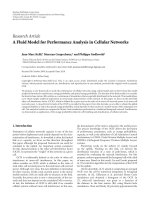
like configuration. This can be understood by analyzing the
driving-point (DP) plot of the system. The derivative of the

state value is plotted in function of the state value in Figure 1.
The state equation of a cell can be divided in two parts, one
depending on the state value of the cell, g(x
i,j
(t)), and the
other part depending only on the neighbors:
dx
i,j
(t)
dt
= g

x
i,j
(t)

+ w(t), (8)
dx
ij
/dt
A(i, j; i, j)
= 1
x
ij
1−1
w
Figure 1:TheDPplotofacell.Thederivativeofthestatevalueis
presentedinfunctionofthestatevalue,forw(t)
= 0 (continuous
line) and w(t) > 0 (dashed line).

where
g

x
i,j
(t)

=−
x
i,j
(t)+A(i, j; i, j)∗f

x
i,j
(t)

,
w(t)
=

k,l
/
=i,j
A
i,j;k,l
y
k,l
(t)+bu
i,j
.

(9)
Becausewehaveacoupledtemplateinwhichw(t)changes
in time, also the DP plot of the system changes in function
of w(t)(inFigure 1 the case of w(t)
= 0 is plotted with a
continuous line, and w(t) > 0 is represented with dashed
line). We cannot predict the exact final steady state of the
cell, but we can see that the equilibrium points cannot be
in the (
−1, 1) region, so the output of the cell will be always
±1. The single exceptions will be the cells (spins) with 0 local
energy, in which case w(t)
= 0. It can happen that these cells
do not achieve a
±1 output (although on real hardwares, in
presence of real noise this is hardly probable), but the state of
these does not affect the energy of the Ising configuration. So
we can just randomly choose between
−1and 1. The result
given by the CNN is similar to finding more than one state at
the same time.
We can conclude thus, that starting from any initial
condition, the final steady state of the CNN template will
be always a local minimum of the spin-glass type Ising
spin system with local connections defined by matrix A.
The fact that one single operation is needed for finding a
local minimum of the energy gives us hope to develop fast
optimization algorithms.
4. The Optimization Algorithm
As already emphasized, the complex frustrated case (locally

coupled spin-glass-type system), where the A coupling
parameters generate a nontrivial quenched disorder will be
considered here. The minimum energy configuration of such
systems is searched by an algorithm which is similar to the
well-known simulated annealing method [24].
The noise is included with random input images (u
i,j
values in (5)) acting as an external locally variable magnetic
field. The strength of this field is governed through parameter
4 EURASIP Journal on Advances in Signal Processing
Start
Read connection matrix: A
i
= 1
b
= b
0
Generate initial condition, a random
binary image: X
Generate input U: random binary
image with 1/2 probability
UX
Run CNN template:
{A, b}
b =b − Δb
Y
X
= Y
Ye s
b>0?

Save Y, calculate the energy
No
No
i
= n?
i
= i +1
Ye s
End
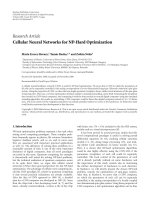
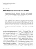
Figure 2: Flowchart of the optimization algorithm using n number
of cooling processes.
b. Whenever b is different from zero, our CNN template
minimizes the energy with form (5).Thefirstpartofit
being the energy of the considered spin-glass-type model
and the second part an additional term, which gets minimal
when the state of the system is equal to the input image (the
external magnetic field). If b is large, the result will be the
input image itself, if b
= 0 the result is a local minimum
of the pure Ising-type system. For values in between, our
result is a “compromise” between the two cases. Slowly
decreasing the value of b will result in a process similar with
simulated annealing, where the temperature of the system is
consecutively lowered. First, big fluctuations of the energy
are allowed, and by decreasing this we slowly drive the system
to a low-energy state. Since the method is a stochastic one, we
can, of course, never be totally sure that the global minimum
will be achieved, but good approximations can be achieved.
The algorithm is as follows (see Figure 2).
(1) One starts from a random initial condition x,andb

=
5 (with this value the result of the template is almost
exactly the same as the input image).
(2) A binary random input image u is generated with 1/2
probability of black (1) pixels.
(3) Using the x initial state and the u input image, the
CNN template is applied.
(4) The value of b is decreased with steps Δb.
(5) Steps 2–4 are repeated until b
= 0isreached.
The results of the previous step (minimization) are
considered always as the initial state for the next step.
(6) When reaching b
= 0, the image (Ising spin
configuration) is saved and the energy is calculated.
In the classical-simulated annealing algorithm, several
thousands of steps for a single temperature are needed. Here,
at each noise value one single CNN template is applied. The
settling time of the template may vary (it is usually longer in
the beginning and gets very fast at the end of the algorithm),
but given the fact that after each step noise is introduced, it
is acceptable to set a constant running time for our template
(usually 5 times the time constant of the CNN dynamics).
Similarly, with choosing the cooling rate in simulated
annealing, choosing the value of Δb is also a delicate prob-
lem. A proper value providing an acceptable compromise
between the quality of the results and speed of the algorithm
has to be found. For each system size, one can find an optimal
value of Δb, but as one would expect this is rapidly decreasing
by increasing the system size. It is much more effective, both

for performance (meaning the probability of finding the real
global optimum) and speed to choose a constant Δb
= 0.05
step and repeat the whole cooling process several times. As
a result, several different final states will be obtained, and
we have a higher probability to get the right global minima
between these. On the flowchart, the number of cooling
processes is denoted with n (Figure 2).
For testing the efficiency of the algorithm, one needs to
measure the number of steps necessary for finding the right
global minima. To do this, one has to previously know the
global minima. In case of small systems with L
= 5, 6 this
can be obtained by a quick exhaustive search in the phase
space. For bigger systems, the classical-simulated annealing
algorithm was used. The temperature was decreased with a
rate of 0.99 (T
final
/T
ini
) and 1000 Monte Carlo steps were
performed for each temperature.
In the present work, spin-glass systems with A(i, j; k, l)
=
±
1, local connections were studied. The P probability
of the positive bonds was varied (influencing the amount
of frustration in the system), and local interactions with
the 8 Moore neighbors were considered. For several P
densities of the positive links and various system sizes, we

calculated the average number of steps needed for finding the
energy minimum. As naturally is expected for the nontrivial
frustrated cases, the number of simulation steps needed
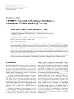
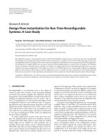
exponentially increases with the system size. As an example,
the P
= .4 case is shown in Figure 3(a). As observable in the
figure, we could made estimates for relatively small system
sizes only (L<12). The reason for this is that we had to
simulate also the CNN operations, and for large lattices a
huge system of partial differential equations had to be solved.
This process gets quite slow for bigger lattices.
The needed average number of steps to reach the
estimated energy minima depends also on the P probability
EURASIP Journal on Advances in Signal Processing 5
4 5 6 7 8 9 10 11 12
L
100
1000
Number of steps
n = c
∗
exp(aL), c = 5.982, a = 0.501
(a)
00.20.40.60.81
p
0
50
100
150
200

250
Number of steps
(b)
Figure 3: (a) The number of steps needed to find the optimal energy as a function of the lattice size L. The density of positive connections is
fixed to P
= .4, and the parameter Δb = 0.05 is used. (b) For a system with size L = 7, the number of steps needed for getting the presumed
global minima is plotted as a function of the probability of positive connections p.
4681012
L
0.001
0.01
0.1
1
10
Time (s)
CNN
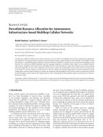
SA
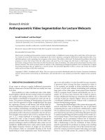
Figure 4: (a) Time needed to reach the minimum energy as a
function of the lattice size L. Circles are for estimates on CNN
computers and squares are simulated annealing results on 3.4 GHz
Pentium 4. Results are averaged on 10 000 different configurations
with P
= .4 probability of positive bonds. For the CNN algorithm,
Δb
= 0.05 was chosen. For simulated annealing, the initial
temperature was T
0
= 0.9, final temperature T
f
= 0.2, and the

decreasing rate of the temperature was fixed as 0.99.
of the positive connections in the system. In Figure 3(b),we
illustrate this for a system with size L
= 7. To obtain this data
for each P-value, 5000 different systems were analyzed. As
observable in Figure 3(b), the system is almost equally hard
to solve for all P-values in the rage of P
∈ (0, .6).
On real hardwares, one has to think about the fact
that noise appears also in the template values, and it may
introduce small asymmetries (A(i, j; k, l)
= A(k, l; i, j)will
be only approximative). We also tested this case in our
simulations. For P
= .4 density of the positive connections
and for 7
× 7 lattice size, 1000 systems were analyzed,
introducing a relatively large 10% noise on the template
values. Results show no significant difference, the average
value of the number of steps needed was 264.0, while in
the symmetric case, for the same system size this average
was 265.8. Given the fact that our algorithm is similar to
simulated annealing, and noise is introduced in the system
at each step, these small asymmetries may only increase the
noise, but have no significant effect.
5. Speed Estimation
Finally, let us have some thoughts about the estimated speed
of such an optimization algorithm. On the CNN chips
nowadays available, only parameter z can be locally varied,
parameters A and B are 3

×3 matrices, uniformly applied for
all cells [6]. The reason for no local control of A and B seems
to be more due to the lack of motivations. It is technically
possible, of course, that the control unit and template
memories of the CNN-UM would be more complicated. This
modification would not change too much the properties of
the hardwares. Introducing the connection parameters (the
template) in the local memories of the chip would take a
longer time, but in the specific problem considered here the
6 EURASIP Journal on Advances in Signal Processing
connection parameters have to be introduced only once for
each problem, so this would not effect in a detectable manner
the speed of calculations.
Based on our previous experience with the ACE16K
chip (with sizes 128
× 128) [14, 15], we can make a rough
estimation of the speed for the presented optimization
algorithm. This chip with its parallel architecture solves one
template in a very short time—of the order of microseconds.
For each step in the algorithm, one also needs to generate a
random binary image. This process is already 4 times faster
on the ACE16K chip than on a 3.4 GHz Pentium 4 computer
and needs around 100 microseconds (see [14]). It is also
helpful for the speed that in the present algorithm it is not
needed to save information at each step, only once at the
end of each cooling process. Saving an image takes roughly 1
millisecond on the ACE16K, but this is done only once after
several thousands of simulation steps. Making thus a rough
estimate for our algorithm, a chip with similar properties like
the ACE16K should be able to compute between 1000–5000

steps in one second, independently of the lattice size. Using the
lower estimation value (1000 steps /second) and following up
the number of steps needed in case of P
= .4, the estimated
average time for solving one problem is plotted as a function
of the lattice size in Figure 4 (circles).
Comparing this with the speed of simulated annealing
(SA) performed on a 3.4 GHz Pentium 4 (squares in
Figure 4), the results for larger lattice sizes are clearly in favor
of the CNN chips. For testing the speed of simulated anneal-
ing, we used the following parameters: initial temperature
T
0
= 0.9, final temperature T
f
= 0.2, decreasing rate of the
temperature 0.99. Results were averaged for 10 000 different
bond distributions. The necessary number of Monte Carlo
steps was always carefully measured by performing many
different simulations, using different number of Monte Carlo
steps, and comparing the obtained results. From Figure 4,
it results that the estimated time needed for the presented
algorithm on a CNN chip would be smaller than simulated
annealing already at 10
×10 lattice sizes.
Spin-glass-like systems have many applications in which
global minimum is not crucial to be exactly found, the
minimization is needed only with a margin of error. In
such cases, the number of requested steps will decrease
drastically. As an example in such sense, it has been shown

that using spin-glass models as error-correcting codes, their
cost performance is excellent [23], and usually the system is
not even in the spin-glass phase. In this manner, by using the
CNN chip, finding acceptable results could be very fast, even
on big lattices.
6. Conclusion
A cellular neural network with locally variable parameters
was used for finding the optimal state of locally coupled, two-
dimensional, Ising-type spin-glass systems. By simulating the
proposed optimization algorithm for a CNN chip, where all
connections can be locally controlled, very good perspectives
for solving such NP hard problems were predicted. CNN
computers could be faster than digital computers already
at a 10
× 10 lattice size. Chips with 2 layers of cells
were also produced (CACE1k [25]) and increasing the
number of layers is expected in the near future. This way,
achieving local control could further extend the number of
possible applications. On two layers, it is possible to map
already a spin system with any connection matrix (even
globally coupled spins) and similar stochastic optimization
algorithms could be developed, and also other important
NP-hard problems (e.g., K-SAT) may become treatable.
Acknowledgments
This work is supported by a Hungarian ONR Grant no.
(N00014-07-1-0350) and a Romanian Consiliul National al
Cercetarii Stiintifice din Invatamantul Superior (CNCSIS)
no.1571 research Grant (Contract 84/2007).
References
[1] H. Nishimori, Statistical Physics of Spin Glasses and Informa-

tion Processing: An Introduction, Clarendon Press, Oxford, UK,
2001.
[2] T. Roska, “Computational and computer complexity of ana-
logic cellular wave computers,” in Proceedings of the 7th IEEE
International Workshop on Cellular Neural Networks and Their
Applications (CNNA ’02), pp. 323–338, Frankfurt, Germany,
July 2002.
[3] L. O. Chua and T. Roska, “The CNN paradigm,” IEEE
Transactions on Circuits and Systems I, vol. 40, no. 3, pp. 147–
156, 1993.
[4] L. O. Chua and L. Yang, “Cellular neural networks: theory,”
IEEE Transactions on Circuits and Systems, vol. 35, no. 10, pp.
1257–1272, 1988.
[5] T. Roska and L. O. Chua, “The CNN universal machine: an
analogic array computer,” IEEE Transactions on Circuits and
Systems II, vol. 40, no. 3, pp. 163–173, 1993.
[6] A. Rodr
´
ıguez-V
´
azquez, G. Li
˜
n
´
an-Cembrano, L. Carranza, et
al., “ACE16k: the third generation of mixed-signal SIMD-
CNN ACE chips toward VSoCs,” IEEE Transactions on Circuits
and Systems I, vol. 51, no. 5, pp. 851–863, 2004.
[7]
´

A. Zar
´
andy and C. Rekeczky, “Bi-i: a standalone ultra high
speed cellular vision system,” IEEE Circuits and Systems
Magazine, vol. 5, no. 2, pp. 36–45, 2005.
[8] .
[9]T.Roska,L.O.Chua,D.Wolf,T.Kozek,R.Tetzlaff,andF.
Puffer, “Simulating nonlinear waves and partial differential
equations via CNN—part I: basic techniques,” IEEE Transac-
tions on Circuits and Systems I, vol. 42, no. 10, pp. 807–815,
1995.
[10] T. Kozek, L. O. Chua, T. Roska, et al., “Simulating nonlinear
waves and partial differential equations via CNN—part II:
typical examples,” IEEE Transactions on Circuits and Systems
I, vol. 42, no. 10, pp. 816–820, 1995.
[11] J. M. Cruz and L. O. Chua, “Application of cellular neural
networks to model population dynamics,” IEEE Transactions
on Circuits and Systems I, vol. 42, no. 10, pp. 715–720, 1995.
[12] K. R. Crounse, T. Yang, and L. O. Chua, “Pseudo-random
sequence generation using the CNN universal machine with
applications to cryptography,” in Proceedings of the 4th IEEE
International Workshop on Cellular Neural Networks and Their
Applications (CNNA ’96), pp. 433–438, Seville, Spain, June
1996.
EURASIP Journal on Advances in Signal Processing 7
[13] K. R. Crounse and L. O. Chua, “Methods for image processing
and pattern formation in Cellular Neural Networks: a tuto-
rial,” IEEE Transactions on Circuits and Systems I, vol. 42, no.
10, pp. 583–601, 1995.
[14] M. Ercsey-Ravasz, T. Roska, and Z. N

´
eda, “Perspectives for
Monte Carlo simulations on the CNN universal machine,”
International Journal of Modern Physics C,vol.17,no.6,pp.
909–922, 2006.
[15] M. Ercsey-Ravasz, T. Roska, and Z. N
´
eda, “Stochastic sim-
ulations on the cellular wave computers,” European Physical
Journal B, vol. 51, no. 3, pp. 407–411, 2006.
[16] S. F. Edwards and P. W. Anderson, “Theory of spin glasses,”
Journal of Physics F, vol. 5, no. 5, pp. 965–974, 1975.
[17] D. Sherrington and S. Kirkpatrick, “Solvable model of a spin-
glass,” Physical Review Letters, vol. 35, no. 26, pp. 1792–1796,
1975.
[18] F. Barahona, “On the computational complexity of Ising spin
glass models,” Journal of Physics A, vol. 15, no. 10, pp. 3241–
3253, 1982.
[19] S. Istrail, “Statistical mechanics, three-dimensionality and NP-
completeness. I. Universality of intractability for the partition
function of the Ising model across non-planar lattices,” in
Proceedings of the 32nd Annual ACM Symposium on Theory of
Computing (STOC ’00), pp. 87–96, Portland, Ore, USA, May
2000.
[20] M. Mezard, G. Parisi, and M. A. Virasoro, Spin Glass Theory
and Beyond, World Scientific, Singapore, 1987.
[21] G. Rowe, Theoretical Models in Biology: The Origin of Life, the
Immune System, and the Brain, Clarendon Press, Oxford, UK,
1997.
[22] R. N. Mantegna and H. E. Stanley, An Introduction to Econo-

physics: Correlations and Complexit y in Finance, Cambridge
University Press, Cambridge, UK, 2000.
[23] N. Sourlas, “Spin-glass models as error-correcting codes,”
Nature, vol. 339, no. 6227, pp. 693–695, 1989.
[24] S. Kirkpatrick, C. D. Gelatt Jr., and M. P. Vecchi, “Optimiza-
tion by simulated annealing,” Science, vol. 220, no. 4598, pp.
671–680, 1983.
[25] T. Roska and
´
A. Rodr
´
ıguez-V
´
azquez, “Toward visual micro-
processors,” Proceedings of the IEEE, vol. 90, no. 7, pp. 1244–
1257, 2002.