Báo cáo hóa học: " Research Article Wavelet Transform for Processing Power Quality Disturbances" pptx

Hindawi Publishing Corporation
EURASIP Journal on Advances in Signal Processing
Volume 2007, Article ID 47695, 20 pages
doi:10.1155/2007/47695
Research Article
Wavelet Transform for Processing Power Quality Disturbances
S. Chen and H. Y. Zhu
School of Elect rical and Electronic Eng ineering, Nanyang Technolog i cal University, 50 Nanyang Avenue, Singapore 639798
Received 29 April 2006; Revised 25 January 2007; Accepted 17 February 2007
Recommended by Irene Y. H. Gu
The emergence of power quality as a topical issue in power systems in the 1990s largely coincides with the huge advancements
achieved in the computing technology and information theory. This unsurprisingly has spurred the development of more so-
phisticated instruments for measuring power quality distur bances and the use of new methods in processing and analyzing the
measurements. Fourier theory was the core of many traditional techniques and it is still widely used today. However, it is increas-
ingly being replaced by newer approaches notably wavelet transform and especially in the post-event processing of the time-varying
phenomena. This paper reviews the use of wavelet transform approach in processing power quality data. The strengths, limitations,
and challenges in employing the methods are discussed with consideration of the needs and expectations when analyzing power
quality disturbances. Several examples are given and discussions are made on the various design issues and considerations, which
would be useful to those contemplating adopting wavelet transform in power quality applications. A new approach of combining
wavelet transform and rank correlation is introduced as an alternative method for identifying capacitor-switching transients.
Copyright © 2007 S. Chen and H. Y. Zhu. This is an open access article distributed under the Creative Commons Attribution
License, which permits unrestricted use, distribution, and reproduction in any medium, provided the original work is properly
cited.
1. INTRODUCTION
Power quality is an umbrella terminology covering a mul-
titude of voltage disturbances and distortions in power sys-
tems [1, 2]. It is often taken as synonymous to voltage qual-
ity as electr ical equipment is generally designed to operate
on voltage supply of certain “quality.” However, “quality” is
a subjective matter as it depends very much on the individ-
ual requirements and circumstances. Voltage that is consid-

ered good for operating water heater may not be adequate
for powering computers. In essence, power quality is a com-
patibility issue between the supply systems and loads [3].
As long as both can coexist without causing any ill effects
on each other, the quality can be regarded as good or ade-
quate. Hence, the scope of power quality is often extended
to include imperfections in the design of supply system such
as unbalanced transmission/distribution lines, poor connec-
tions, and inapt groundings.
Nonetheless, the majority of disruptions recognized as
power quality problems involve electromagnetic phenomena
that cause the supply voltage to deviate from its ideal char-
acteristics of constant frequency (50/60 Hz), constant volt-
age m agnitude (nominal values), and completely sinusoidal
[1]. These phenomena can be divided into two broad cat-
egories of time-varying and steady-state (or intermittent)
events. The former group comprises voltage transients, dips,
swells, and interruptions. They normally occur for a brief
period of time (several milliseconds), but are often severe
enough to cause wide-ranging disruptions to many electrical
loads. Voltage dips lasting 5-6 cycles are known to cause pro-
grammable logic controller (PLC) in factories to malfunc-
tion. The latter group includes voltage unbalances, harmonic
and interharmonic distortions, voltage fluctuation, notch-
ing, and noise. These steady-state (or semi-steady-state) phe-
nomena would act subtly over a certain period of time be-
fore disruption occurs or intolerable condition surfaces. Har-
monic voltage causes additional stress on equipment insu-
lation, shortening their useful life. The eventual insulation
breakdown often occurs after the equipment is being sub-

jected to the distort ion over extended period of time.
Signal processing is generally called upon when there is
a need to extract specific information from the raw data,
which typically in power systems are the voltage and cur-
rent waveforms. The objectives of collecting data through
measurements or simulations largely dictate which signal
processing technique is to be utilized [4]. In power quality
context, an evaluation often involves several phases that can
be broadly divided into problem identification, classification
2 EURASIP Journal on Advances in Signal Processing
and character isation, followed by solution assessment and
design. Further processing may be necessary if the results
are to be presented in some special way. Designer of power
conditioner would need to know the worst-case distur-
bance/distortion levels with much detailed, and both the
magnitude and phase angle are equally important for the
conditioner operation. On the other hand, a facility manager
evaluating the overall quality level would prefer an overview
of the measurements incorporating some statistical sum-
maries. In such cases, magnitude would probably be suffi-
cient. Regulator monitoring customers’ compliance to limits
would need the data processed and the results presented ac-
cording to the methods stipulated in the regulation, standard
or contract. Althoug h one can argue that similar techniques
can be applied in all scenarios, but the degree of processing
or summarization is often different, largely affected by the
length of the evaluation period.
With the advancement in measurement technology, an
increasing volume of data is being g a thered and it needs
to be analyzed. It is highly desirable if the analysis is auto-

mated. Signal processing is therefore called upon for identi-
fication, classification and characterization. The techniques
used vary, depending on the characteristics of the phenom-
ena. As power systems use AC (alternating current), the RMS
(root-mean-square) quantity is the most commonly used
measure for voltage magnitude. Although it is meant for
periodic waveform, it is often taken as a rough estimate of
the nonperiodic or time-varying voltage variations. Voltage
dips, swells, and interruptions are often characterized and
classified using this quantity. When more explicit informa-
tion is needed, such as evaluating disturbance propagation,
time-frequency decomposition methods are necessary. Dis-
crete Fourier transform (DFT) is a convenient way of visual-
izing stationary a nd periodic signal from its frequency con-
tent viewpoint. It is also applied to nonstationary signals but
with added windowing to focus on cer tain per iod of time.
This is called short time Fourier transform (STFT), allowing
some tracing of the magnitude variations. Harmonic distor-
tions are typically handled in this manner but the constraint
placed on the frequency resolution makes it difficult to ex-
tend STFT to the analysis of interharmonics.
Fast voltage transients require the peak magnitudes and
rise times to be determined accurately. For oscillatory tran-
sient, its predominant frequency needs to be derived before
computing its magnitude. DFT is often used even though
these waveforms are not periodic and last for less than one
fundamental cycle since it is often necessary to determine
their spectra content. Estimation techniques such as Kalman
filtering are also called upon when there are uncertainties
in the data. For other analyses that consider the effect of

sensitive loads such as flickering of incandescent lamp due
to voltage fluctuation, the data processing needs to mimic
the behavior of lamp responses, human visual and psy-
chological perception. Finally, after identification, classifica-
tion, and characterization, the relevant information needs
to be stored for future reference. Although the signal pro-
cessing undertaken in these steps can be taken as some
form of compression, further processing and threshold op-
eration is often car ried out to reduce the amount of data
stored.
Wavelet transform (WT) is increasingly being proposed
for the above processing in place of Fourier-based tech-
niques. The primary reason for advocating WT is that it does
not need to assume that the signal is stationar y or periodic,
not even within the analysis window. This makes it highly
suitable for tracing changes in signal including fast changes
in high-frequency components. WT is a time-scale decom-
position technique and is generalized as a form of time-
“frequency band” analysis method. It not only traces sig-
nal changes across the time plane, but it also breaks signal
up across the frequency plane. In discrete wavelet t ransform
(DWT), signal is broken into multiple frequency bands, in-
stead of a discrete number of frequency components as in
DFT. With this character, WT is more appropriate if one is
unsure of the exact frequency. Fortunately, most analyses do
not require the exact frequency since a lumped quantity (fre-
quency band) is sufficient to achieve their purposes. How-
ever, with power system engineering heavily entrenched in
Fourier’s techniques, it remains questionable if wavelet tech-
niques are applicable and useful for the representation and

analysis of voltage disturbances encountered in power sys-
tems [5].
This paper reviews the wavelet t ransform as a signal
processing tool for processing power-quality-related distur-
bance waveforms. Section 2 provides a succinct introduction
of WT and dwells into the properties of its basis functions.
It explains the flexibilities and options inherent in the WT
procedure, and demonstrates how they can be employed in
power quality analysis. The challenges as well as opportu-
nities presented by this new signal processing technique are
traded side-by-side with respect to the requirements in ana-
lyzing power quality data. In Section 3,someexemplaryuses
of WT in power quality studies are presented. This is fol-
lowed by Section 4 detailing various important factors that
must be considered when contemplating wavelet approach
in power quality applications. Section 5 describes a new ap-
proach of combining rank correlation with WT for identify-
ing the capacitor-switching event. The conclusions and rec-
ommendations are given on which power quality phenom-
ena WT i s suitable for use and vice versa.
2. WAVELET ANALYSIS
Wavelet analysis is a technique for carving up function or
data into multiple components corresponding to different
frequency bands. This allows one to study each component
separately. The main idea existed since the early 1800s when
Joseph Fourier first discovered that signals could be repre-
sented as superposed sine and cosine waves, forming the ba-
sis for the infamous Fourier analysis. From the beginning of
1990s, it began to be utilized in science and engineering, and
has been known to be particularly useful for analyzing sig-

nals that can be described as aperiodic, noisy, intermittent,
or transient [6]. With these traits, it is widely used in many
applications including data compression, earthquake pre-
diction, and mathematical a pplications such as computing
S.ChenandH.Y.Zhu 3
numerical solutions for partial differential equations [7]. In
recent years, it is increasingly being used in many power
system applications including power quality measurement
and assessment [8].
Wavelet analysis is a form of time-frequency technique as
it evaluates signal simultaneously in the time and frequency
domains. It uses wavelets, “small waves,” which are functions
with limited energy and zero average,

+∞
−∞
ψ(t)dt = 0. (1)
The functions are typically normalized,
ψ=1 and cen-
tered in the neighborhood of t
= 0. It plays the same role
as the sine and cosine functions in the Fourier analysis. In
wavelet transform, a specific wavelet is first selected as the
basis function commonly referred to a s the mother wavelet.
Dilated (stretched) and translated (shifted in time) versions
of the mother wavelet are then generated. Dilation is denoted
by the scale parameter a while time translation is adjusted
through b [9],
ψ
a,b

(t) =
1
√
a
ψ

t − b
a

,(2)
where a is a positive real number and b is a real number. The
wavelet transform of a signal f (t) at a scale a and time trans-
lation b is the dot product of the signal f (t) and the partic-
ular version of the mother wavelet, ψ
a,b
(t). It is computed by
circular convolution of the signal with the wavelet function
W

f (a, b)

=

f , ψ
a,b

=

+∞
−∞

f (t) ·
1
√
a
ψ
∗

t − b
a

dt.
(3)
A contracted version of the mother wavelet would corre-
spond to high frequency and is typically used in temporal
analysis of signals, while a dilated version corresponds to low
frequency and is used for frequency analysis.
With wavelet functions, only information of scale a<1
corresponding to high frequencies is obtained. In order to
obtain the low-frequency information necessary for full rep-
resentation of the original signal f (t), it is necessary to deter-
mine the wavelet coefficients for scale a>1. This is achieved
by introducing a scaling function φ(t) which is an aggre-
gation of the mother wavelets ψ(t) at scales greater than 1.
The scaling function can also be scaled and translated as the
wavelet function,
φ
a,b
(t) =
1
√

a
φ

t − b
a

. (4)
With scaling function, the low-frequency approximation of
f (t) at a scale a is the dot product of the signal and the par-
ticular scaling function [9], and can be computed by circular
convolution
L

f (a, b)

=

f , φ
a,b

=

+∞
−∞
f (t)
1
√
a
φ
∗


t − b
a

dt. (5)
Implementation of these two transforms (3)and(5)canbe
done smoothly in continuous wavelet transform (CWT) or
discretely in discrete wavelet transform (DWT). The details
are descr ibed in Appendix A.
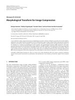
2.1. Multiresolution analysis
One important trait of wavelet transform is that its nonuni-
form time and frequency spreads across the frequency plane.
They vary with scale a but in the opposite manner, with
the time spread being directly proportional to a while fre-
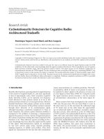
quency spread to 1/a.Thiseffect is best illustrated by the
time-frequency boxes as shown in Figure 1 for short time
Fourier transform (STFT) and DWT. In STFT, the time and
frequency resolutions (Δt and Δ f ) are constant as illust rated
by the fixed square boxes over the time-frequency plane.
On the other hand, the resolutions of DWT vary across the
planes. At low frequency when the variation is slow, the time
resolution is coarse while the frequency resolution is fine.
This enables accurate tracking of the frequency while allow-
ing sufficient time for the slow variation to transpire before
analysis. On the contrary, in the high-frequency range, it is
important to pinpoint when the fast changes occur. The time
resolution is therefore small, but the frequency resolution is
compromised. However, it is generally not necessary to know
the exact frequency in this range.
It is to be noted that as the resolutions vary, the area

of the time-frequency boxes remain unchanged. This area is
lower-bound by a limit as stipulated by the Heisenberg un-
certainty principle “the more precisely the position is deter-
mined, the less precisely the momentum is known in this
instant and vice versa.” This principle asserts that one can-
not know the exact time-frequency representation of a sig-
nal (i.e., what spectral components exist at what instants of
time). What one can know is the time interval in which cer-
tain band of frequencies exists, which is a resolution prob-
lem. In DWT, this principle still holds but it is manipulated
to achieve the optimal time and frequency resolutions at dif-
ferent frequency ranges.
This adjustment of the resolutions is inherent in wavelet
transform as the wavelet basis is stretched or compressed
during the transform. A high scale corresponds to a more
“stretched” wavelet having a longer portion of the signal be-
ing compared with it. This would result in the slowly chang-
ing coarser feature of the signal to be determined accurately.
On the contrary, a low scale uses compressed wavelet to sift
out rapidly changing details that correspond to high frequen-
cies. Compressed wavelet provides the necessary precision
time resolution while compromising the frequency resolu-
tion. This a bility to expand function or signal with differ-
ent resolutions is termed as multiresolution analysis, which
forms the cornerstone of many w avelet applications.
Armed with this capability, wavelet tr a nsform is used in
many applications including signal suppression where cer-
tain parts are suppressed to highlight the remaining por-
tion. The highlighted portion can either be low or high fre-
quency. Another popular application is denoising where it is

used to recovering signal from samples corrupted by noise.
This is very effective when the noise energy is concentrated
in different scales from those of the signal. In addition, the
relative scarceness of wavelet representation allows unneces-
sary information to be discarded without compromising the
original intent. This is heavily exploited in data compression
4 EURASIP Journal on Advances in Signal Processing
STFT
f
t
Δt
= N
1
f
s
Δ f =
f
s
N
DWT
f
t
Δt
= a · N
1
f
s
Δ f =
1
a

·
f
s
4
Figure 1: Comparison of time and frequency resolutions ( f
s
: sampling frequency; N: number of sample points per analysis window).
especially in the storage and handling of images. Last but not
least, the localization property of wavelet enables discontinu-
ities or breakdown points to be easily and vividly identified. It
is therefore widely applied for detection of the onset of cer-
tain events and to pin down the exact instant of the occur-
rence. Section 3 describes several power quality applications
that make use of these capabilities.
3. WAVELET APPLICATIONS IN POWER QUALITY
The ability of wavelet transform in segregating a signal into
multiple frequency bands with optimized resolutions makes
it an attractive technique for analyzing power quality wave-
form. It is particularly attractive for studying disturbance or
transient waveform, where it is necessary to examine differ-
ent frequency components separately. This section discusses
several popular uses of wavelet transform in the analysis of
power quality disturbances.
3.1. Characterization of voltage transients
The time and space localization property of wavelet trans-
form makes it highly suitable for analysis of discontinuities
or abrupt changes in signal. In power systems, there are
many voltage transients due to lightning strikes, equipment
switching, load turning-on, and faults. With multiresolution
analysis, the DWT provides a logarithmic coverage of the

frequency spectrum as depic ted in Figure 1.Thishasbeen
shown to be useful in characterizing voltage transients caused
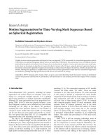
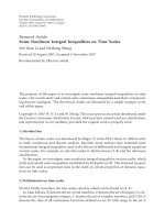
by capacitor switching and faults [10]. Figure 2 shows how
two voltage transient waveforms can be expanded into vari-
ous levels (scales) corresponding to several frequency bands.
In level 1, which is the highest frequency, several short bursts
are observed for capacitor switching. Compared to the two
distinct and separated bursts for fault, this can be used as
the discriminating feature between the events. In addition,
significant ringing is observed at level 4, which may be the
system natural frequency that is significantly affected by the
switched capacitor.
In the above example [10], there is no redundant in-
formation being used in the analysis as only one low-
frequency scale (highest scale) is used alongside the other
high-frequency scales. This corresponds to one approxima-
tion term A
j0
and multiple detail terms D
j
as defined in
Figure 14,where j
0
is the total number of decomposition lev-
els. However, some redundancies may be useful as they may
give more obvious discriminating patterns. In [11], all the
approximation terms A
j
in successive decomposition levels
are also employed alongside the detail terms D

j
to form the
discriminating patterns between fault t ransient and capacitor
switching transient.
Similar wavelet expansion approach is also being pro-
posed for analyzing current drawn by arc furnace [12]. The
wavelet expansion helps to identify which frequency ranges
the disturbance energy is concentrated. The same technique
is also applied to inrush, fault, and load currents for differ-
entiating between transformer magnetization inrushes, in-
ternal short circuit faults, internal incipient faults as well as
external short circuit faults and load changes [13]. The re-
constructed bands of signals from wavelet coefficients in the
respective scales form the unique patterns necessary for dis-
crimination.
3.2. Characterization of short-duration
voltage variations
Short-dur ation voltage variations, namely, dips, swells, and
interruptions are commonly encountered in power systems.
Turning on large loads such as induction motors or faults
are known to cause these voltage variations that badly affect
S.ChenandH.Y.Zhu 5
Capacitor switching transient
2
0
−2
v(t)
0 1020304050607080
0.2
0

−0.2
Level 1
0 1020304050607080
0.2
0
−0.2
Level 2
0 1020304050607080
0.2
0
−0.2
Level 3
0 1020304050607080
0.2
0
−0.2
Level 4
0 1020304050607080
2
0
−2
Approx.
0 1020304050607080
(a)
Fault transient
2
0
−2
v(t)
020406080

0.2
0
−0.2
Level 1
020406080
0.2
0
−0.2
Level 2
020406080
0.2
0
−0.2
Level 3
020406080
0.2
0
−0.2
Level 4
020406080
2
0
−2
Approx.
020406080
(b)
Figure 2: Wavelet expansion of voltage transients.
the operation of m any modern electronic equipment. The
important characteristics that indicate their severity are the
magnitude and duration of the variations. Traditionally,

RMS computation is used to derive the magnitude while the
duration is taken as the time period the RMS magnitude stays
below/above certain threshold (< 90% for dips and > 110%
for swells. Although RMS method is generally considered as
sufficient, the wavelet approach has been shown to produce
more accurate results that would be useful for determining
the causes of such variations.
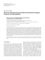
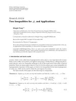
Figure 3 shows the waveform of a short-duration volt-
age dip (70%; 5 cycles) followed by a 10-cycle interruption
in (a), and the corresponding characterization using wavelet
method. First, (b) and (c) shows the use of CWT in sift-
ing out two frequency components of 50 Hz and 650 Hz and
constructing their respective profiles [14]. The 650 Hz profile
shows several sharp peaks denoting discontinuities, which
are the occurring or ending instants of the disturbances. They
are used to determine the durations of the dip and inter rup-
tion. On the other hand, the 50 Hz profile shows magnitude
of the dip and interruption, respectively. It can be shown that
this approach works well too for very short voltage variation
with duration less than half a cycle.
This method has also been suggested for analyzing high-
frequency oscillatory transients. CWT is used to isolate the
1500 Hz component and if its profile shows sharp and short
peaks, then the disturbance is one of the voltage variations.
If it shows a long series of peaks, then it corresponds to high-
frequency transients. The same argument can also be applied
to the 650 Hz component for low-frequency transients.
Instead of CWT, it is more efficient to employ DWT with-
out many compromises to the characterization accuracy. The
multiresolution analysis capability of DWT ensures that fine

time resolution is maintained at the high-frequency bands
for determining the occurring and ending instants. Although
the time resolution at the low-frequency band loses preci-
sion, it is not used to determine the times and hence it is still
sufficient to approximate the magnitude variations. This is
illustrated by (d) and (e). (d) is the DWT detail coefficients,
which contain the high-frequency details with fine time reso-
lution for pinpointing the time instants, while (e) is the DWT
approximation coefficients reflecting the magnitude change.
3.3. Classification of various power quality events
The different levels of wavelet coefficient over the scales can
be interpreted as uneven distribution of energy across the
multiple frequency bands. This distribution forms patterns
that have been found to be useful for classifying between dif-
ferent power quality events. If the selected wavelet and scaling
functions form an orthonormal (independent and normal-
ized) set of basis, then the Parseval theorem relates the energy
of the signal to the values of the coefficients. This means that
the norm or energy of the signal can be separated according
to the following multiresolution expansion:



f (t)


2
dt =

k



A
j
0
(k)


2
+

j≤j
0

k


D
j
(k)


2
. (6)
These squared wavelet coefficients were shown to be use-
ful features for identifying power quality events. In [15], the
6 EURASIP Journal on Advances in Signal Processing
2
0
−2

0 100 200 300 400 500
(a) Voltage waveform
0.4
0.2
0
0 100 200 300 400 500
(b) CWT 650 Hz profile
1
0.5
0
0 100 200 300 400 500
(c) CWT 50 Hz profile
1
0
−1
0 100 200 300 400
(d) DWT level 4 coefficients
5
0
−5
0 100 200 300 400
(e) DWT approx. coefficients
Figure 3: Char acterization of a short-duration voltage dip.
statistics of these values are used to identify transformer en-
ergization, converter operation, capacitor energizing and re-
striking. The maximum value of the squared coefficients in
each scale or its average is found to be different before, dur-
ing, and after transformer energization. Changes in these val-
ues are used as the feature for its identification. Similarly,
converter operation results in voltage notches, which are

treated as discontinuities by wavelet transform and shown up
in the high-frequency scales. Counting the number of high-
valued squared coefficients over one fundamental period
would lead to the event. Capacitor energization or breaker
restriking on opening are known to cause rather dramatic
voltage steps. When processed using DWT, high squared co-
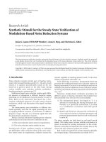
efficients are found across various scales. Figure 4 shows a
capacitor energizing transient waveform and the correspond-
ing squared coefficients for three detail levels. The maximum
values in each of the levels can be used as the feature to rec-
ognize the event. In [16], the averages or selections of coef-
ficients are used as inputs to a self-organizing mapping neu-
ral network to distinguish between transients caused by load
switching and capacitor switching.
Instead of using the maximum or average values, the
energy distribution pattern in the wavelet domain can be
computed as sums of the squared coefficients as in (6).
1
0
−1
Volt a ge ( p u)
0 1020304050607080
0.02
0.01
0
Squared wavelet
coefficients
0 1020304050607080
Level 1
0.02

0.01
0
Squared wavelet
coefficients
0 1020304050607080
Level 2
0.04
0.02
0
Squared wavelet
coefficients
0 1020304050607080
Level 3
Time (ms)
Figure 4: Capacitor-switching transient waveform and squared
wavelet coefficients.
Figure 5 shows this energy distribution pattern for several
commonly encountered power quality events. Differences
between these patterns provide the differentiation features.
Isolated capacitor switching shows more energy being dis-
tributed among the lower levels, corresponding to higher fre-
quencies than the back-to-back switching. This reflects the
differences between the high-frequency transients in the for-
mer condition and the low-frequency transients in the lat-
ter. Impulsive transient shows energy being generally con-
fined to the highest frequency band (level 1). The pattern for
voltage dip shows energy in the low-frequency region (level
5), which includes the fundamental frequency. However, the
transients at the starting and ending instants manifest them-
selves as energy components in other lower scales (levels 3

and 4). These transients are not as pronounce when energiz-
ing transformer. Often, there are some uncertainties with the
waveforms or patterns due to the varying system and com-
ponent parameters. Hence, fuzzy reasoning is used to extend
the identification rules derived from these energy distribu-
tion patterns [17]. Probabilistic neural network is another
possible approach but it requires significant amount of data
for training [18, 19].
4. WAVELET METHOD DESIGN ISSUES
The success of applying wavelet transform in various applica-
tions depends very much on several crucial design decisions.
First, these decisions certainly have to be based on the objec-
tives of the analysis. Although there can be many contrasting
requirements, the bottom line can be narrowed to how accu-
rate one can anticipate the nature of the analyzed signal. In
S.ChenandH.Y.Zhu 7
4
2
0
12345
Wavelet expansion levels
back-to-back capacitor
switching transient
4
2
0
Isolated capacitor
switching transient
12345
Wavelet expansion levels

0.4
0.2
0
Voltage dip
12345
Wavelet expansion levels
0.4
0.2
0
Lightning impulsive transient
12345
Wavelet expansion levels
0.4
0.2
0
Transformer energization inrush
12345
Wavelet expansion levels
0.1
0.05
0
Pure sine wave
12345
Wavelet expansion levels
Figure 5: Energy distribution pattern in wavelet domain for various
power quality events.
time-frequency decomposition, it is usually how exact one
can anticipate the frequency contents of a signal that influ-
ences the choice of technique, the associated design settings,
and the subsequent implementation. For wavelet transform,

these are the choice of mother wavelet, CWT or DWT, and
the number of expansion levels.
4.1. Selection of mother wavelet
Successful application of wavelet transform depends heavily
on the mother wavelet. The most appropriate one to use is
generally the one that resembles the form of the signal. This
is particularly true for achieving good data compression ra-
tio since a close resemblance would produce high coefficients
in cer tain selective scales and near-zero coefficients in the re-
maining scales. However, this may not necessarily be as use-
ful when forming patterns for identification and classifica-
tion. Unique pattern for each event is more important than
confining the coefficients to certain scales. Typically, if the
representation can be spread across multiple scales, it tends
to reduce the dependency on specific scales and thus helps to
desensitize the identification and classification process. This
would also make the process more robust and reduce erro-
neous identification.
There is a wide range of mother wavelets to choose from
and each of them possesses unique properties as described
in Appendix B. For power quality applications, it has been
quoted to preferably be oscillatory, with a short support and
has at least one vanishing moment [11, 19]. The oscillatory
feature is trivial as power networks are ac and many phenom-
ena including transients are oscillatory in nature. A short
support is a good trait as it keeps the number of high co-
efficients small. In addition to having less data to operate on,
it also makes it easier to set thresholds for detection. Van-
ishing moments is another useful quality to have as it helps
to suppress regular part of the signal, highlighting the sharp

transitions. Unfortunately, support size and number of van-
ishing moments often go hand-in-hand and a compromise is
necessary. Generally, most power quality applications would
select a mother wavelet with short support but has one or
two vanishing moments.
Among the several wavelet functions that were men-
tioned in the literature, the Daubechies family of wavelets are
the most widely used [12, 13, 15–18]. This is perhaps due to
its wavelets satisfying the necessary properties as described
in the previous paragraph. Daubechies wavelets are also well
known and widely used in other applications. It is flexible
as its order can be controlled to suit specific requirements.
Among the different dbN (N-order) wavelets, db4 is the
most widely adopted wavelet in power quality applications.
It has sufficient number of vanishing moments to bring out
the transients while maintaining a relatively short support
to avoid having too many high-valued coefficients. Choos-
ing the right mother wavelet often requires several rounds
of trials, depending very much on the designer’s experience
and knowledge of the signal to be analyzed. Oftentimes, only
subtle differences are observed from using one wavelet to an-
other. The lack of explicit expressions for many wavelet func-
tions also makes it difficult to compare them with mathemat-
ical rigours. Sometimes, it is the implementation issues such
as the efficient DWT computation via FIR filtering that con-
stitutes the overriding factor.
4.2. CWT or DWT
DWT can be viewed as a subset of CWT. This, on the out-
set, seems to favour CWT but as this is a redundant trans-
formation, too much information may derail the identifica-

tion and classification process. Hence, in the above illustra-
tive examples, only one example uses CWT [14], while the
others are all using DWT to take advantage of its provision
of multiresolution analysis. In multiresolution analysis, the
DWT process decomposes a signal into a discrete number
of logarithmic frequency bands as shown on the left-hand
side of Figure 6 [10]. At each level of decomposition or fil-
tering and downsampling, the signal bandwidth is split into
two halves of high and low frequencies. The low-frequency
half is split further in subsequent decomposition or filtering.
8 EURASIP Journal on Advances in Signal Processing
Level 1
Level 2
Level 3
Level 4
Level 5
Level 6
Approx. level
Wavelet expansion levels
5kHz
2.5kHz
1.25 kHz
625 Hz
312.5Hz
156.25 Hz
78.125 Hz
0Hz
Nyquist frequency for
10 kHz sampling rate
High-frequency transients

System-response
transients
Characteristic
harmonics
Fundamental frequency
Figure 6: Frequency division of DWT filter for 10 kHz sampling
rate.
This rather rigid way of splitting the frequency bandwidths
may pose some difficulties to certain applications.
On the right-hand side of Figure 6, the typical power
quality phenomena of interest are listed [10]. Despite the
rather rigid division in frequency, DWT is still deemed fit if
the events of interest can be localized to within one or two
bands. At high frequencies, the frequency bandwidths are
wide leading to poor frequency resolutions. It can be seen
that the high-frequency transients fall within a bandwidth
between 2 kHz and 3 kHz and further processing is necessary
to determine the predominant frequency if it is oscillatory.
The wide bandwidth also admits many frequencies, mak-
ing the filtering less selective at the high-frequency range.
Therefore, if knowing specific frequency component is im-
portant, CWT or Fourier method is more suitable than DWT.
However, if only an aggregate information within certain fre-
quency bands are needed, DWT would be a more convenient
and efficient choice.
4.3. Number of decomposition levels
The number of decomposition or expansion levels is very
much related to the selection of CWT or DWT. For CWT,
there is no rigid manner of decomposition, and hence the
number of levels is arbitrary and as required. Frequently, it

is decided according to the center frequency of the selected
mother wavelet. For the CWT example shown in Figure 3,
scales of 256 and 19.7 are selected for the 50 Hz and 650 Hz
components, for using a complex mother wavelet cmor1–1.5
(center frequency of 1) and sampling rate of 12.8 kHz (256
samples per fundamental cycle). On the other hand, with
limited levels in DWT, it has to be decided carefully and it
depends on how many divisions are to be made to the low-
frequency ranges. Four to five levels of decomposition seem
to be the most popular [13, 15–17], while some use seven to
eight levels [10, 12], or even as many as thirteen levels [18].
In N DWT decomposition levels, there will be N
− 1detail
levels and 1 approximation level. Most applications use both
the detail and approximation levels but some use only the de-
tail levels. The approximation level is almost always used to
trace the fundamental frequency component only.
4.4. Wavelet or Fourier
It is inevitable that the wavelet techniques would be com-
pared to the popular Fourier techniques. The Fourier the-
ory is deeply entrenched in many areas of power system en-
gineering, and this leads to a “risk” or “trap” that wavelet
techniques are used to represent or mimic Fourier-based ex-
pressions. Fourier techniques rely on relatively good knowl-
edge of the sig nal spectrum. The design of measurement
and processing systems are heavily dependent on this knowl-
edge. Otherwise, spectral leakage can be significant leading to
the need for windowing, which adds to the implementation
complexity.
In discrete Fourier transform (DFT), the window length

hasapronounceeffect as it determines the frequency resolu-
tion. The evaluated coefficients are basically magnitude and
phase angle of each discrete frequency component. Wavelet
techniques on the other hand are form of time-frequency
analysis with predefined or accompanied windowing. Its co-
efficients denote information contained within successive
bands of frequency. It is more forgiving for any slip-up in
anticipating the frequency content of the signal. Therefore,
it can be gener alized that wavelet method is attractive when
one is not absolutely certain about the frequencies that make
up the sig nal. This is often the situation for voltage transient
and wavelet methods are strongly advocated for analyzing
transient signals with abrupt changes.
4.5. Wavelet for harmonic and interharmonic analysis
The ability to segregate between frequencies also leads to pro-
posals to use wavelet transform in the analysis of harmonics
and interharmonics. However, as these phenomena by defi-
nitions are sinusoids, it is always questionable if it is sensi-
ble to represent them using other basis functions besides the
customary sine and cosine functions. Wavelet transform with
some time information does possess the ability to track vari-
ations. However, it is arguable that this tracking can also be
achieved through windowing such as in STFT.
To analyze harmonic and interharmonic distortion prob-
lems, it is necessary to know individual or groups of harmon-
ics and interharmonics. In IEC Standard 61000-4-7 [20], a
window length of 10 (or 12) cycles is recommended for use in
50 (or 60) Hz power systems, producing frequency-domain
representations in 5 Hz bins. These 5 Hz bins are then com-
bined to produce harmonic and interharmonic groupings

and components for which compatibility levels and limits are
specified.
As5Hzresolutionisrequiredatbothhigh-andlow-
frequency ranges, DWT is not suitable. An adapted ver-
sion, called wavelet packet transform ( WPT), can be used as
the high-frequency details coefficients are also decomposed
further at each subsequent level. This effectively creates a
series of bandpass filters w ith relative similar bandwidths
across the entire frequency plane. With proper selection of
S.ChenandH.Y.Zhu 9
mother wavelet and number of decomposition levels, this
approach has been shown to produce comparable results as
those using DFT [21]. However, the design and implemen-
tation can be rather complex and it has yet to be proven
to bring about much advantage when compared to DFT.
In addition, harmonics and interharmonics are character-
istically defined as sinusoids, making DFT the more con-
venient method, especially when results are to be checked
against standard or guideline. Specifically, wavelet transform
can be employed to track their variation, but as these phe-
nomena are normally considered as steady-state or quasi-
steady-state, the usual DFT is an equally effective analysis
method.
5. WAVELET TRANSFORM AND RANK CORRELATION
FOR IDENTIFICATION OF CAPACITOR-SWITCHING
TRANSIENTS
Among the many voltage disturbances in power systems, os-
cillatory transients caused by capacitor switching are com-
monly encountered as capacitors are used to improve the
customers’ load power factor or for utility voltage support.

These transients typically take the form of underdamped re-
sponse as follows:
V(t)
= A
0
· sin

2πf
0
t + ϕ
0

+ e
−α
1
t
· A
1
· sin

2πf
1
t + ϕ
1

+ e
−α
2
t
· A

2
· sin

2πf
2
t + ϕ
2

+ ···,
(7)
where the subscript 0 denotes the fundamental frequency,
and the remaining subscripts refer to the oscillatory tran-
sients. Each transient component is characterized by its
amplitude A
x
, oscillating frequency f
x
, and damping fac-
tor α
x
.
These characteristics are often used to identify and de-
tect capacitor sw itching. The oscillating frequency and mag-
nitude variation were used to determine the size and lo-
cation of the shunt capacitor [22]. In [15], Santoso used
the typical frequency and the variation of step voltage af-
ter switching to characterize capacitor switching transient.
Despite these past efforts, differentiating capacitor switching
transients from other disturbances remains a challenge. This
is because the transient behaviour depends considerably on

the system conditions and the capacitor. Particularly, v aria-
tions in system conditions and capacitor power ratings alter
these characteristics, posing challenges to measurement and
detection techniques that focus on these quantities. Wavelet
techniques, with their bandpass property, are therefore more
robust than Fourier methods as they are less frequency selec-
tive. The transient amplitude and the manner it decays away
are heavily affected by the system and component variations.
This impact can be largely nullified by using other measures
such as the ranks instead of the absolute magnitudes of the
captured transient waveform. This section introduces the use
of rank correlation for analyzing the underdamped response
of the transient component as a mean to identify capacitor-
switching events.
5.1. Extracting the transient component
Energizing a capacitor bank t ypically results in two major
transient components, inrush transient and energizing tran-
sient. The former is due to an initial downward surge of the
voltage as the charged system capacitance tries to transfer its
charges to the uncharged capacitor. This transient can be sig-
nificant when turning on large capacitors and it also occurs
when turning on loads that are fitted with power factor cor-
rection capacitor. This inrush transient is typically of high
frequencies in tens of kHz, making it difficult to measure.
Hence, it is not commonly used for identification. In addi-
tion, capacitors are often fitted with 1 mH inductance to limit
this inrush, affecting the measurement.
After the initial inrush, the system would eventually
charges up the combined capacitance. This charging causes
another voltage and current surge, cumulating to the ener-

gizing transient. It is oscillatory but damped out gradually
by the system resistance. Unlike inrush transient, it is more
substantially affected by the system conditions. Its frequency
is much lower, at around 1 kHz, and it can be readily mea-
sured and used for identification. However, finding the exact
frequency is difficult unless all of the system par a meters are
known. Even if relying on prior knowledge of the system or
past measurements, it is more practical to estimate the prob-
able frequency range. This then requires an analysis method
that is not heavily dependent on having precise information
on this frequency. Wavelet methods fit this requirement as
they are band-limited filters and not confined to any specific
frequency.
In this method, CWT is preferred over DWT due to its
more flexible frequency selec tion. DWT, with its dyadic cal-
culation structure, confines its scale and frequency band to
discrete values, making it difficult to contain a ll transient in-
formation within a single band for identification. The center-
frequency of a CWT scale is adjusted to match as closely as
possible to the expected dominant frequency of the ener-
gizing transient. In addition, with its inherent redundancy,
the time resolution is maintained ensuring sufficient data is
available in all bands for use in the identification.
Once the dominant frequency is trapped, its magnitude
variation e
−α
1
t
· A
1

is reflected by the change in the energy
content of the particular frequency band. Such information
on the voltage V
c
(t) at a particular scale s
c
and time instant
t
0
can be obtained using the following expressions:
W

V
c

t
0
, s
c

=

+∞
−∞
V
c
(t)
1
√
s

c
ψ
∗

t − t
0
s
c

dt
=

V
c
, ψ
t
0
,s
c

= V
c
∗ ψ
s
c

t
0

.

(8)
The corresponding energy density at this scale and at this
time instant can be calculated as
P
W

t
0
, s
c

=


W

V
c

t
0
, s
c



2
. (9)
With this energy density definition, the energy from half a
cycle of the voltage waveform, which indirectly reflects the

10 EURASIP Journal on Advances in Signal Processing
magnitude of this band, is
E
W

s
c
, t
0

=

t
0
+T
1
/2
t
0
P
W

t, s
c

dt=

t
0
+T

1
/2
t
0


W

V
c

t, s
c



2
dt,
(10)
where T
1
is the period of the oscillatory transient. By sliding
the computation window over time, changes in the energy
content reflects the magnitude variation. The magnitude of
this energy varies with its initial value A
1
, which depends
among many parameters on the point-on-wave when the ca-
pacitor is switched.
5.2. Rank correlation

Rank correlation is a kind of nonparametric statistical meth-
od that evaluates the similarity between two signals through
their ranks. It is used here to evaluate the similarity between
the variation in the transient amplitude and that of a prede-
fined signature waveform. The correlation gives a value close
to 1 if they match, verifying that the disturbance is similar to
the signature. Instead of comparing the absolute magnitudes,
rank correlation evaluates whether the shape of a signal fits
that of another signal. This method is immune to the mea-
surement methods as it only concerns with the shape and
not on the actual value. It is easy to implement and appear
to be a good choice for comparing the amplitude variation
of capacitor-switching transients. There a re two main types
of rank correlation methods, the Spearman and the Kendall
[23], and the former is used in this method.
Spearman rank correlation is a distribution-free analogy
of correlation analysis. It compares two independent ran-
dom variables, each at several levels (which may be discrete
or continuous). It judges whether the two variables covary
(i.e., vary in similar direction) or as one variable increases,
the other variable tends to increase or decrease. Spearman
rank correlation works on ranked (relative) data. The smal l-
est value is replaced with a 1, the next smallest with a 2, and
so on. It measures the nonlinear relationship or the similarity
between two variables despite their different magnitudes. It is
suitable for use with skewed data or data with extremely large
or small v alues. Ties are assigned if some variables have iden-
tical values, and the average of their adjacent ranks is used in
the comparison. With “ties,” the Spearman rank correlation
coefficient is calculated as

ρ
s
=

1 −
6
N
3
− N

N

i=1

R
i
− S
i

2
+
1
12

k

f
3
k
− f

k

+
1
12

m

g
3
m
− g
m




1 −

k

f
3
k
− f
k

N
3
− N


1/2

1 −

m

g
3
m
− g
m

N
3
− N

1/2

,
(11)
where N is the length of the two v ariables; R
i
and S
i
are the
ranks of respective variables; f
k
and g
m

are the number of ties
in the kth or mth group of ties among the R
i
’s or S
i
’s. The co-
Source
Line 1
CAP40
1mH
C40AL C40BL
0.15 mH 0.15 mH
40-MVAr 40-MVAr
TR 1
TR 2
13.8kV
Load 3.8-MVAr
13.8kV
138 kV
E138
Load
Figure 7: Single-line diagram of a 138 kV 60 Hz illustrative system.
efficient ρ
s
indicates agreement. A value near 1 indicates good
agreement while a value near zero or negative, poor agree-
ment.
5.3. Dynamic simulations and verifications
A 138 kV 60 Hz test system as shown in Figure 7 is used to
illustrate this method [24]. Two 40 MVAr capacitor banks

at the 138 kV busbars are used to simulate the two types of
capacitor switching—isolated and back-to-back. The three-
phase fault current at the 138 kV bus is approximately
13.7 kA, giving a short circuit capacity of about 1890.6 MVA.
For the study of switching transient, the test system can be
simplified to a Thevenin equivalent with a series resistance R
s
of 0.58 Ω, series inductance L
s
of 15.39 mH giving X
s
of 5.8 Ω
and X/R ratio of 10. The system stray capacitance is taken to
be 1200 nF and used only in the analysis of isolated switch-
ing. For the back-to-back switching, one of the two 40 MVAr
capacitor banks is assumed to be already connected when the
other one is switched.
Dynamic simulations are carried out using Matlab/
Simulink. The transient waveforms are processed using CWT
followed by rank correlation to identify if they are caused
by capacitor switching. db2 is the mother wavelet due to
its simplicity. With a center-frequency of 0.6667 and sam-
pling frequency of 15.36 kHz, a wavelet scale of 22.8 is se-
lected, giving a pseudofrequency of 449.12 Hz. This is close to
the estimated response frequency of the signature at 450 Hz.
Figure 8 shows the oscillatory transients from the energiza-
tion of a 40 MVAr capacitor. For the signature, it is assumed
that the capacitor is switched at the voltage peak produc-
ing the biggest transient. The corresponding amplitude vari-
ation of the signature and the transients derived using (10)

are shown in Figure 9. Due to the differences in their am-
plitudes, absolute correlation of the phases with the signa-
ture would not produce good agreement. Particularly, phase
A with small transient showing the biggest difference from
the signature would produce a rather l ow coefficient. In
S.ChenandH.Y.Zhu 11
200
100
0
−100
−200
Volt a ge ( k V)
0 5 10 15 20 25 30 35
Time (ms)
Phase A
Phase B
Phase C
Figure 8: Voltage waveforms of a capacitor-switching transient.
140
120
100
80
60
40
20
0
Volt a ge ( k V)
0246810
Time (ms)
Signature

Phase A
Phase B
Phase C
Figure 9: Amplitude variations of signature and transient.
a three-phase system, the instantaneous magnitudes of the
phase voltages are generally different, w i th one phase low,
close to zero while the other two phases much higher. There-
fore, the transient on that particular phase would be much
smaller compared to the other two.
On the other hand, if the ranks of the signature and tran-
sients are compared as shown in Figure 10, the correlation
coefficients are much higher and more consistent. As can be
seen from the graphs, the ranks for the phases very much
coincide with that of the signature despite the amplitude dif-
ferences. Even for phase A with small transient amplitude,
the correlation remains good and much better than the abso-
lute correlation of Figure 9. However, to maintain high accu-
racy, only the two most significant phases are used for iden-
tification. Their average value is compared to some thresh-
old, such as 0.9, to deduce on whether the transient is caused
by capacitor switching. In the following subsections, several
simulations are carried out to verify the robustness of this
wavelet-based rank correlation method.
150
100
50
0
Rank
0246810
Time (ms)

Signature
Phase A
Phase B
Phase C
Figure 10: Ranks of signature and t ransient.
1
0.5
0
−0.5
−1
Volt a ge w avef o rm ( p u)
0246810121416
Time (ms)
Instant 1
Instant 2
Figure 11: Switching instants on phase A voltage waveform.
5.3.1. Effect of different switching instants
Figure 11 shows two point-on-wave instants of one of the
phases when the capacitor is energized. Two sets of simula-
tion results are obtained as shown in Tables 1, 2,and3 for
isolated and back-to-back capacitor switching. For each of
the cases, it is obvious that one phase shows a poorer cor-
relation compared to the other two. The averages shown in
the rightmost column are derived from the two phases with
the highest coefficients. A result close to 1 denotes close re-
semblance to the signature, suggesting that the disturbance is
a capacitor-switching transient. Different switching instants
mean that different instantaneous voltage being impressed
on the uncharged capacitor when it is switched. In addi-
tion, the phases are phase-shifted from each other, causing

the rank correlation results to vary between the phases and
from one instant to another. Nonetheless, two of the phases
always show significant transients that allow the rank cor-
relation method to produce noticeable result, even though
the instants are different from that of the signature at voltage
peak.
12 EURASIP Journal on Advances in Signal Processing
Table 1: Results of isolated capacitor switching.
Capacitor size Switching instant Phase A Phase B Phase C Average of two highest phases
20 MVAr
1 0.786 0.933 0.691 0.860
2 0.956 0.797 −0.362 0.876
40 MVAr
1 0.887 0.989 0.929 0.959
2 0.971 0.967 0.364 0.969
60 MVAr
1 0.897 0.951 0.932 0.941
2 0.956 0.940 0.541 0.948
80 MVAr
1 0.825 0.916 0.886 0.901
2 0.914 0.907 0.493 0.911
Table 2: Results of back-to-back capacitor switching w ith 40 MVAr connected.
Capacitor size Switching instant Phase A Phase B Phase C Average of two highest phases
20 MVAr
1 0.558 0.952 0.747 0.850
2 0.955 0.833 −0.414 0.894
40 MVAr
1 0.712 0.922 0.864 0.893
2 0.918 0.890 −0.006 0.904
60 MVAr

1 0.689 0.847 0.813 0.830
2 0.833 0.842 0.530 0.838
80 MVAr
1 0.649 0.798 0.781 0.789
2 0.771 0.793 0.066 0.782
5.3.2. Effect of different capacitor ratings
Tabl es 1, 2,and3 also show the results of switching capac-
itors of lower and higher ratings than the 40 MVAr used to
generate the signature. Nevertheless, the correlation results
remain high above 0.75, and they are still reasonably good
for identifying capacitor switching. This is because although
different capacitor size would result in different characteristic
frequency, the relative frequency variation is small. In these
cases, the frequency variations are smaller than
±50 Hz in
isolated switching cases and
±100 Hz in back-to-back cases.
These ranges are still very much covered by the selected CWT
bandwidth, producing satisfactory rank correlation results.
The declining trend indicates that the correlation deterio-
rates as the actual system response moves away from that of
the signature. A lower threshold value may be necessary if
there exists such large uncertainties.
5.3.3. Isolated or back-to-back switching
Comparing Tables 2 and 3 to Table 1 , the influence of exist-
ing capacitance in the network can be observed. In Table 2,a
40 MVAr capacitor is assumed to be in service when another
capacitor is switched. In Table 3, the connected capacitor is
assumed to be twice as big at 80 MVAr. Generally, different
responses are expected but the characteristics of these switch-

ing transients tend to overlap in both frequency and time.
Therefore, the selected signature, which is derived from iso-
lated switching of a 40 MVAr capacitor, is still largely effec-
tive for back-to-back switching except for a few conditions
where the size of the switched capacitor also differs from the
40 MVAr used in the signature.
5.3.4. Effects from different system conditions
It is always difficult to be completely certain about all of the
system parameters. Any uncertainty may affect the identifica-
tion accuracy. Ta ble 4 shows the correlation results when the
system inductance is half or double of that used to derive the
signature. The results confirm the robustness of the method
as the rank correlation coefficients remain good, greater than
0.9. Although these variations change the transient damping
time constant from 6 milliseconds to 9 milliseconds, it how-
ever does not affect the performance of the method. Similar
studies were also conducted for different system resistances
and system capacitances, and the correlation remains good.
For the cases on system capacitance, the uncertainties show
weaker impact compared to those from back-to-back switch-
ing. In such cases, the connected capacitor would dominate
the system capacitance and affects the transient characteris-
tics. However, as shown in Tabl e 2, the proposed method is
still applicable albeit needing a lower threshold.
5.3.5. Noncapacitor-switching transients
To further verify the validity of the method, transients caused
by other switching events are also simulated and used to test
its rejection capability. The reactor switching is the energiza-
tion of a 40 MVAr reactor at the 138 kV busbar. The trans-
former switched is rated at 20 MVA 138/3.8 kV, while the

S.ChenandH.Y.Zhu 13
Table 3: Results of back-to-back capacitor switching w ith 80 MVAr connected.
Capacitor size Switching instant Phase A Phase B Phase C Average of two highest phases
20 MVAr
1 0.174 0.781 0.136 0.477
2 0.765 0.672 −0.486 0.718
40 MVAr
1 0.315 0.788 0.751 0.769
2 0.744 0.812 −0.336 0.778
60 MVAr
1 0.477 0.826 0.761 0.794
2 0.800 0.817 −0.298 0.809
80 MVAr
1 0.575 0.841 0.770 0.805
2 0.829 0.826 −0.258 0.827
Table 4: Results with changes to system parameters.
System change Switching instant Phase A Phase B Phase C Average of two highest phases
50% L
s
1 0.847 0.959 0.955 0.957
2 0.941 0.963 −0.008 0.952
200% L
s
1 0.811 0.867 0.903 0.885
2 0.849 0.904 0.213 0.876
50% R
s
1 0.886 0.988 0.935 0.962
2 0.970 0.970 0.369 0.970
200% R

s
1 0.892 0.989 0.916 0.953
2 0.971 0.965 0.369 0.968
50% C
s
1 0.884 0.969 0.907 0.939
2 0.971 0.944 0.399 0.957
200% C
s
1 0.884 0.964 0.939 0.952
2 0.962 0.974 0.282 0.968
Table 5: Results of other disturbances.
Transient events Cases Phase A Phase B Phase C Average of two highest phases
Reactor switching
1 −0.088 0.830 −0.645 0.371
2 0.882 −0.241 −0.595 0.321
Transformer energization
1 −0.036 0.849 −0.667 0.407
2 0.849 −0.282 −0.550 0.284
Line energization
1 −0.060 0.815 −0.604 0.377
2 0.906 −0.097 −0.587 0.404
line energized is 50 km long, both connected to the 138 kV
busbar. The results in Table 5 show low average correlations
that can be easily rejected by setting an appropriate thresh-
old. Generally, the characteristic frequencies of these tran-
sients are not close to that of the capacitor switching. The
rank correlation results would therefore be low or even neg-
ative. For some phases and at certain switching instants, the
correlation appears high at about 0.85. However, closer in-

spection reveals that the transients are very small, and can
be discounted in the first place. The good correlation there
is due to the very low energy content having similar profile
as that of signature. Fortunately, the other two phases show
poor correlation, helping to reject their identification. From
these results, it is illustrated that by selec ting an appropri-
ate threshold such as 0.70, the major ity of these disturbances
can be differentiated from the transients caused by capacitor
switching.
6. CONCLUSIONS
Wavelet transform is quickly becoming the choice method
for processing power quality data. This is due to its ex-
cellent time and frequency localization capability, and the
flexibility in implementation. However, using wavelet trans-
form can be involving, especially at the design stage. The
many flexible features translate into more decisions that need
to be made. Selection of mother wavelet, using CWT or
DWT and the number of decomposition le vels are the three
14 EURASIP Journal on Advances in Signal Processing
most important decisions that can affect its performance sig-
nificantly. Wavelet transform is more forgiving than other
methods when the form of the signal is not clearly known.
It is ideal for handling phenomena with fast changing or
abrupt transients. In this paper, it is shown to be effec-
tive for characterizing and classifying switching transients,
fault transients, and short-duration voltage variations. The
response frequency of these disturb ances tends to fluctuate
with changes in the system but generally remains within cer-
tain band that can be easily covered by wavelet techniques.
These characteristics are exploited in a new capacitor switch-

ing transient identification method. The method adopts the
use of rank correlation in place of the customary absolute
correlation, overcoming several challenges that are brought
about by uncertainties in the system conditions. However,
Wavelet method is found to be not useful for phenomena
whose characteristics are customarily defined using Fourier
or other basis functions, such as harmonics and interhar-
monics. As the understanding of wavelet transform grows,
there will be more attempts at applying it to power quality
analysis but it remains to be seen if it can be as successful on
other issues as on transients.
APPENDICES
A. WAVELET TRANSFORMS
Wavelet transform is carried out by convolving a wavelet with
a signal or function. The wavelet can be manipulated in two
ways: stretched or squeezed (scaled) and moved to various
locations on the sig nal. If it matches the signal well at a spe-
cific scale and location, then a large transform value is ob-
tained. However, if they do not correlate well, a low value en-
sues. The transform is usually computed at various locations
on the signal and at various scales. It is done in a smooth
continuous fashion for the continuous wavelet transform
(CWT) or in discrete steps for the discrete wavelet transform
(DWT).
Compared to other time-frequency analysis, CWT de-
composes signal with less restrict ion on its resolution. It can
operate at any scale, up to the highest scale that is limited
only by the Nyquist sampling theorem [9]. CWT is also con-
tinuous in terms of time shifting. During computation, the
scaled mother wavelet is shifted smoothly over the full do-

main of the signal. Accordingly, a one-dimensional signal is
translated into a two-dimensional time-frequency represen-
tation by the coefficients of CWT. This smooth transition of
the scaled mother wavelet implies that there are many over-
laps in the transform making the CWT representation highly
redundant.
Instead of the highly redundant CWT, DWT is often used
as it is more efficient computationally and requires less mem-
ory storage. Unlike CWT where the expansion is performed
on any arbitrary scale, DWT follows a certain discrete ex-
pansion pattern determined by the selection of a factor a
0
.
The most widely used pattern is called dyadic expansion
with a
0
= 2 and the expansion is implemented for scales
a
= a
j
0
,where j = 1, 2, 3, The information in the high-
frequency bands as carried by the details D
j
is computed
as
D
j
[n] = W


f

a
j
0
, n

=
N−1

m=0
f [m] ·
1

a
j
0
ψ
∗

m − n
a
j
0

,
(A.1)
where N is the total number of samples of the ana-
lyzed signal. Similarly, the information in the low-
frequency band as carried by the approximations

A
j
are coefficients of DWT with the scaling func-
tion
A
j
[n] = L

f

a
j
0
, n

=
N−1

m=0
f [m] ·
1

a
j
0
φ
∗

m − n
a

j
0

.
(A.2)
A.1. Frequency responses of wavelet and
scaling functions
The stretching or compressing of wavelet and scaling func-
tions to derive h igh- and low-frequency information is akin
to filtering through a highpass filter and a lowpass filter. In-
deed, wavelet and scaling functions can be interpreted as im-
pulse responses of highpass and lowpass filters, respectively.
Figure 12 shows a widely used mother wavelet, db2 and
its Fourier transforms for several normalized scales. They
resemble the frequency responses of bandpass filters. The
bandwidth and center frequency of each pass band v ary with
the scale a. At low scale, corresponding to high frequency,
the pass band is wide with high center frequency. As a in-
creases and approaches 1, the center frequency reduces and
the bandwidth becomes narrower too, as the frequency re-
sponse shifts to the left. This demonstrates that the frequency
resolution or localization becomes better towards the low fre-
quencies.
The frequency response of the scaling function φ can
be interpreted as the impulse response of a lowpass filter.
The companion s caling function of db2 wavelet function is
shown in Figure 13 alongside its Fourier transforms for vari-
ous normalized scales. It clearly shows a lowpass charac teris-
tics but the bandwidth and cut-off frequency reduce as scale
a approaches infinity.

These frequency responses demonstrate the different role
played by wavelet function at extracting high-frequency in-
formation and that of scaling function at deriving low-
frequency information. Appendix B describes the implemen-
tation of DWT through successive steps of highpass and low-
pass filtering with filters constructed from the wavelet and
scaling functions, respectively. Normally, multiple wavelet
functions would be used to separate hig h frequencies into
multiple bands while a single scaling function is used to rep-
resent the remaining low-frequency component. The high-
frequency bands are considered as the detailed information
while the low-frequency band is taken as the approximate in-
formation.
S.ChenandH.Y.Zhu 15
2
1.5
1
0.5
0
−0.5
−1
−1.5
ψ
00.511.522.53
(a)
1
0.9
0.8
0.7
0.6

0.5
0.4
0.3
0.2
0.1
0
Normalized magnitude of |ψ|
00.20.40.60.81
ω/π
a  1
(b)
Figure 12: (a) db2 mother wavelet and (b) its Fourier transforms at
various scales.
A.2. Fast implementation of DWT
Recognizing the above frequency responses, the dyadic DWT
decomposition is often implemented as a cascaded high-
pass and lowpass filtering with downsampling as shown in
Figure 14. The highpass filter h[n] is determined from both
the wavelet and scaling functions, while the lowpass filter
g[n] is determined from the scaling function only
h[n]
=

1
√
2
ψ

t
2


, φ( t − n)

,(A.3)
g[n]
=

1
√
2
φ

t
2

, φ( t − n)

. (A.4)
The highpass filtering produces the details D
j
(high fre-
quency) of the decomposition, while the lowpass filtering
produces the approximations A
j
(low frequency). First, the
original signal is passed through the two filters producing the
detail D
1
and approximate A
1

coefficients for j = 1 (scale
a
= 2
1
). After downsampling by a factor of 2, the approxi-
1.4
1.2
1
0.8
0.6
0.4
0.2
0
−0.2
−0.4
φ
00.511.522.53
(a)
1
0.9
0.8
0.7
0.6
0.5
0.4
0.3
0.2
0.1
0
Normalized magnitude of |φ|

00.20.40.60.81
ω/π
a 
∞
(b)
Figure 13: (a) Scaling function of db2 and (b) its Fourier trans-
forms at various scales.
mate coefficients A
1
are passed through the same filters again
to obtain the coefficients for j
= 2 (scale a = 2
2
). After
another downsampling, the approximate coefficients A
2
are
then filtered again to obtain the next level of coefficients. This
filtering operation can be taken as successive segregations of
the same function f , with each segregation providing incre-
mental information for a particular frequency band.
In this way, a given signal f (t) is expanded in terms of its
orthogonal basis of scaling and wavelet functions. In essence,
it is represented by one set of scaling coefficients, and one or
several sets of wavelet coefficients
f (t)
=

k
A

1
(k)φ(t − k)+

k

j=1
D
j
(k)2
−j/2
ψ

2
−j
t − k

=

k
A
j
0
(k)2
−j
0
/2
φ

2
−j

0
t − k

+

k

j≤j
0
D
j
(k)2
−j/2
ψ

2
−j
t − k

,
(A.5)
16 EURASIP Journal on Advances in Signal Processing
Signal f
HP
LP
D
1
A
1
D

2
A
2
HP
LP HP
LP
D
3
A
3
HP
LP
Highpass filter
Lowpass filter
Down-sampling
High
frequencies
Low
frequencies
Figure 14: Fast DWT decomposition.
where A
1
is the scaling coefficient as computed from (A.2)
while D
j
is the j-level wavelet coefficients computed from
(A.1). k denotes the translation in time and scales j denote
the different frequency bands, from high to low frequencies
for j
= 1, 2, TheycanbecomputedviaDWTfiltersof

(A.3)and(A.4) as follows:
A
j+1
(k) =

n
h(n − 2k)A
j
(n),
D
j+1
(k) =

n
g(n − 2k)A
j
(n).
(A.6)
B. FAMILIES OF WAVELET FUNCTIONS
One reason for the popularity of wavelet technique is the vast
choices of wavelets as the basis function, compared to the
fixed choice of sine and cosine functions for Fourier analy-
sis. This enables wavelet analysis to be adapted according to
the expected characteristics of the signal. A coarse (irregu-
lar) wavelet is more suitable for signal with sharp or abrupt
transitions, while those smooth ones are better analyzed us-
ing regular wavelets. Figure 15 shows some commonly u sed
wavelet functions and their associated scaling functions plot-
ted on their immediate left. Each function possesses own
unique properties that lend them to be more appropriate for

certain range of applications. Some of the essential properties
are listed and explained below.
(i) Support size: the speed of convergence to zero as time
or the frequency goes to infinity, which quantifies both
time and frequency localisations.
(ii) Symmetry : useful in avoiding dephasing in image pro-
cessing.
(iii) Number of vanishing moments: useful for compres-
sion purposes as it separates smooth and transient
parts of the signal.
(iv) Regularity: useful for getting nice features, like
smoothness of the reconstructed signal or image, and
for the estimated function in nonlinear reg ression
analysis.
(v) Presence of scaling function: needed for representing
the low frequencies.
The effectiveness of CWT and DWT is influenced by the
choice of mother wavelet and its scaling function, if it exists.
Different types of mother wavelets have different properties.
There are many wavelet functions and they can be divided
into three types according to their orthogonality, namely,
redundant wavelets, orthogonal wavelets, and biorthogonal
wavelets. Orthogonal and biorthogonal wavelets analysis lead
to no redundancy. In addition, biorthogonal wavelets have
an added advantage as their filters are symmetric and can be
used to reconstruct the original signal. However, not all the
properties are significant for power quality applications. The
following sections describe several important properties that
need to be considered when choosing wavelet functions for
power quality applications, which a summary of several pop-

ular wavelet functions is given in Table 6.
B.1. Number of vanishing moments
Awaveletψ is defined to have p vanishing moments if

+∞
−∞
t
k
ψ(t)dt = 0for0≤ k<p,(B.1)
where p and k are integers. This means that ψ is orthogonal
to an y p
−1 degree polynomial. Therefore, if a signal has reg-
ular part whose degree of order is less than p
−1, the regular
part can be readily suppressed during wavelet transform. For
a signal f (t) that is continuously differentiable at point zero,
it can be expanded into the following Taylor expansion series:
f (t)
=

f (0) + tf

(0)
+ t
2
f
(2)
(0) + ···+ t
p−1
f

(p−1)
(0)

+ g(t),
(B.2)
where g(t) is the irregular part of the sig nal f (t). As p
−1de-
gree polynomial would be suppressed by wavelet transform,
both g(t)andf (t) would have the same detail coefficients.
This means that with sufficient number of vanishing mo-
ments, wavelet transform would systematically suppress the
S.ChenandH.Y.Zhu 17
Haar
1.5
1
0.5
0
−0.5
−1
−1.5
00.511.50 0.511.5
1.5
1
0.5
0
−0.5
−1
−1.5
db2
1.4

1.2
1
0.8
0.6
0.4
0.2
0
−0.2
−0.4
01230123
2
1.5
1
0.5
0
−0.5
−1
−1.5
Meyer
1.2
1
0.8
0.6
0.4
0.2
0
−0.2
−0.4
−10 −50 5 10 −10 −50 5 10
1.5

1
0.5
0
−0.5
−1
Coif2
1.4
1.2
1
0.8
0.6
0.4
0.2
0
−0.2
0 5 10 15 0 5 10 15
2
1.5
1
0.5
0
−0.5
−1
Figure 15: Some popular wavelet functions and respective scaling functions.
regular parts of a signal and would focus on the irregular
parts [9, 25, 26]. This would help to reveal the irregular parts
and is very useful when processing transient signals.
B.2. Support size
Support size quantifies the localization in time and fre-
quency. If the analyzed signal has a nondifferentiable point

that falls within the support of a wavelet function, there
maybemanyhighwaveletcoefficients. Hence, to keep the
number of nonzero coefficients low, it is normally advis-
able to keep the support size small. However, the wavelet
functions used are often orthogonal wavelets, whose support
size always increases or decreases in tandem with the num-
ber of vanishing moments. For an orthogonal wavelet hav-
ing p vanishing moments, its support size is at least 2p
− 1
[9, 27]. As a larger number of vanishing moments are gen-
erally preferred for signal suppression purpose, there needs
to be a trade-off between the number of vanishing moments
and the support size. Although it helps to identify transients
or abrupt changes, the subsequent large support size would
result in many high coefficients. In general, if a signal is
highly irregular, it would be better to decrease the support
size at the cost of reducing the number of vanishing mo-
ments.
B.3. Regularity
The regularit y of wavelet function has mostly a cosmetic
influence on the error introduced by thresholding of the
wavelet coefficients. If the function is r-time continuously
differentiable (r is a nonnegative integer), then its regular-
ity is r. A large r implies a more regular function. For cer-
tain wavelet functions such as the Daubechies wavelets, the
regularity is linked to the support s ize. The longer the sup-
port a Daubechies wavelet has, the more regular the func-
tion is. Regularity is useful in estimating the local properties
of a function or signal. With a regular mother wavelet, the
18 EURASIP Journal on Advances in Signal Processing

Table 6: Summary of wavelet families.
Properties
Morlet
(morl)
Mexican-hat
(mexh)
Meyer
(meyr)
Haar
(Haar)
Daubechies
(dbN)
Gaussian
(gaus)
Symlet
(symN)
Coiflet
(coifN)
Biorthogonal
wavelet pairs
(biorNr.Nd)
Regularity Infinitely Infinitely Infinitely No Arbitrary Infinitely Arbitrary Arbitrary Arbitrary
Compactly
supported
orthogonal
No No No 2 2N − 1No2N− 16N− 12
Nd
+1
Symmetry Yes Yes Yes Yes Asymmetry Yes
Near

symmetry
Near
symmetry
Yes
Number of
vanishing moments
———1N—N2NNr− 1
Existence of scaling
function
No No Yes Yes Yes No Yes Yes Yes
Orthogonal analysis No No Yes Yes Yes No Yes Yes No
Biorthogonal analysis
No No Yes Yes Yes No Yes Yes Yes
FIR filters (length)
No No No 2 2N No 2N 6N Yes
Fast algorithm
No No No Yes Yes No Ye s Ye s Ye s
CWT
Yes Ye s Yes Yes Yes Yes Yes Yes Yes
DWT
No No Yes Yes Yes No Yes Yes Yes
Explicit expression
Yes Yes No Yes No Yes No No For splines
reconstructed signal is smooth. It is important to take note
of this property if reconstruction is necessary.
B.4. Symmetry
Symmetric wavelets show no preferred direction or empha-
sis in time, while asymmetric wavelets give unequal weight-
ing to different directions. If a wavelet function is symmet-
ric, it is easier to deal with the boundaries of the signal, be-

cause the phase shift caused by this wavelet function is lin-
ear. Compared to nonlinear phase shift, linear phase shift is
generally more acceptable, especially in image processing. If
the mother wavelet is not symmetric, the wavelet transform
of the mirror of an image is not the mirror of the image’s
wavelet transform. In power quality assessment, the influ-
ence of the signal border distortion of the signal can be miti-
gated by using symmetric mother wavelets [28].
B.5. Choosing mother wavelet
To choose a suitable mother wavelet, the properties of the
wavelet function must be considered carefully. Generally, the
objective of the wavelet analysis and the characteristic of the
analyzed object decide the mother wavelet. If a signal has
a few isolated singularities and is very regular between the
singularities, a wavelet with many vanishing moments can
be chosen to produce mainly small coefficients. If there are
many singularities, it would be better to decrease the sup-
port size at the cost of lower number of vanishing moments.
Wavelet analysis that overlaps the singularities of a signal
would create high coefficients. Furthermore, if signal recon-
struction is needed, a more regular wavelet is preferred in
order to obtain a smoother reconstructed signal. Finally, if
the analysis is to be carr ied out on some specific frequencies,
the center-frequency of the wavelet, the sampling frequency
of the signal, and the length of the signal must be taken into
consideration simultaneously. The selection can be done in
two steps [29].
Step 1 (Determine the wavelet type). If a fast algorithm is
needed, the wavelet must be achievable via FIR filters. If the
approximation part of the analysis is needed, scaling function

becomes necessar y. If reconstruction is needed, biorthogo-
nalwaveletshavesomeadvantagescomparedtoorthogonal
wavelets. The symmetry and exact reconstruction are both
possible with biorthogonal wavelet functions. These require-
ments help to narrow the selection to one of the following
four categories.
Or thogonal wavelets with FIR filters
Thesewaveletscanbedefinedthroughascalingfilter.Pre-
defined families of such wavelets include Haar, Daubechies,
Coiflet,andSymlet.
Biorthogonal wavelets with FIR filters
These wavelets can be defined through two scaling filters for
reconstruction and decomposition, respectively. The Bior-
Splines wavelet family is a predefined family of this category.
S.ChenandH.Y.Zhu 19
Or thogonal wavelets without FIR filter, but with
scaling function
These wavelets can be defined through the definition of a
wavelet function and a scaling function. The Meyer wavelet
family is a predefined family of this category.
Wavelets without FIR filter and without scaling function
These wavelets can be defined through the definition of a
wavelet function only. Predefined families of such wavelets
include Morlet and Mexican
hat.
Step 2 (Define the orders of wavelet within a selected fam-
ily). Some wavelet families have a single wavelet function
such as Haar, Meyer,andMorlet, while some have many such
as Daubechies and Coiflet. If the selected wavelet function is
from the latter group, the order of the selected wavelet func-

tion must be decided. This involves looking at their proper-
ties including the number of vanishing moments, regularity
and support size.
In addition, not all wavelet functions have a scaling func-
tion equivalent. Hence, only those with scaling function can
represent low-frequency information in the wavelet domain.
The others would have only high-frequency representation.
In addition, many wavelet functions like the Daubechies fam-
ily of wavelets do not have explicit expression. Hence, it is
necessary to construct the wavelet and scaling functions in
ordertoevaluatetheirperformance.
REFERENCES
[1] IEC 61000-2-1, “Electromagnetic compatibility (EMC)—part
2: environment - section 1: descr iption of the environment
- electromagnetic environment for low-frequency conducted
disturbances and signalling in public power supply systems,”
1st edition, 1990.
[2] IEEE Std. 1159-1995, “IEEE Recommended Practice for Mon-
itoring Electric Power Quality,” 1995.
[3] IEC 61000-2-2, “Electromagnetic compatibility (EMC)—part
2-2: environment - compatibility levels for low-frequency
conducted disturbances and signalling in public low-voltage
power supply systems,” 2nd edition, 2002.
[4] I. Y H. Gu and E. Styvaktakis, “Bridge the gap: signal pro-
cessing for power quality applications,” Electric Power Systems
Research, vol. 66, no. 1, pp. 83–96, 2003.
[5] I. Y H. Gu and M. H. J. Bollen, “Time-frequency and time-
scale domain analysis of voltage disturbances,” IEEE Transac-
tions on Power Delivery, vol. 15, no. 4, pp. 1279–1284, 2000.
[6] A. Bruce, D. Donoho, and H Y. Gao, “Wavelet analysis [for

signal processing],” IEEE Spectrum, vol. 33, no. 10, pp. 26–35,
1996.
[7] A. Graps, “An introduction to wavelets,” IEEE Computational
Science & Engineering, vol. 2, no. 2, pp. 50–61, 1995.
[8]R.M.C.Fern
´
andez and H. N. D. Rojas, “An overview of
wavelet transforms in power system,” in Proceedings of the 14th
Power System Computational Conference (PSCC ’02), Sevilla,
Spain, June 2002.
[9] S. Mallat, A Wavelet Tour of Signal Processing, Academic Press,
San Diego, Calif, USA, 2nd edition, 1999.
[10] D. C. Robertson, O. I. Camps, J. S. Mayer, and W. B. Gish Sr.,
“Wavelets and electromagnetic power system transients,” IEEE
Transactions on Power Delivery, vol. 11, no. 2, pp. 1050–1056,
1996.
[11] M. Karimi, H. Mokhtari, and M. R. Iravani, “Wavelet based
on-line disturbance detection for power quality applications,”
IEEE Transactions on Power Delivery, vol. 15, no. 4, pp. 1212–
1220, 2000.
[12] W. A. Wilkinson and M. D. Cox, “Discrete wavelet analysis of
power system transients,” IEEE Transactions on Power Systems,
vol. 11, no. 4, pp. 2038–2044, 1996.
[13] K. L. Butler-Purry and M. Bagriyanik, “Characterization of
transients in transformers using discrete wavelet transforms,”
IEEE Transactions on Power Systems, vol. 18, no. 2, pp. 648–
656, 2003.
[14] O. Poisson, P. Rioual, and M. Meunier, “Detection and mea-
surement of power quality disturbances using wavelet trans-
form,” IEEE Transactions on Power Delivery,vol.15,no.3,pp.

1039–1044, 2000.
[15] S. Santoso, W. M. Grady, E. J. Powers, J. Lamoree, and S. C.
Bhatt, “Characterization of distribution power quality events
with Fourier and wavelet transforms,” IEEE Transactions on
Power Delivery, vol. 15, no. 1, pp. 247–254, 2000.
[16] Y Y. Hong and C W. Wang, “Switching detection/classi-
fication using discrete wavelet transfor m and self-organizing
mapping network,” IEEE Transactions on Power Delivery,
vol. 20, no. 2, part 2, pp. 1662–1668, 2005.
[17] T. X. Zhu, S. K. Tso, and K. L. Lo, “Wavelet-based fuzzy reason-
ing approach to power-quality disturbance recognition,” IEEE
Transactions on Power Delivery, vol. 19, no. 4, pp. 1928–1935,
2004.
[18] Z L. Gaing, “Wavelet-based neural network for power dis-
turbance recognition and classification,” IEEE Transactions on
Power Delivery, vol. 19, no. 4, pp. 1560–1568, 2004.
[19] C H. Lin and M C. Tsao, “Power quality detection with clas-
sification enhancible wavelet-probabilistic network in a power
system,” IEE Proceedings: Generation, Transmission and Distri-
bution, vol. 152, no. 6, pp. 969–976, 2005.
[20] IEC 61000-4-7, “Electromagnetic compatibility (EMC)—part
4-7: testing and measurement techniques - gener al guide on
harmonics and interharmonics measurement and instrumen-
tation, for power supply systems and equipment connected
thereto,” International Electrotechnical Commission, 2002.
[21] J. Barros and R. I. Diego, “Application of the wavelet-packet
transform to the estimation of harmonic groups in current
and voltage waveforms,” IEEE Transactions on Power Delivery,
vol. 21, no. 1, pp. 533–535, 2006.
[22] M. M. Saied, “Capacitor switching transients: analysis and

proposed technique for identifying capacitor size and loca-
tion,” IEEE Transactions on Power Delivery,vol.19,no.2,pp.
759–765, 2004.
[23] H. P. William, P. F. Brian, A. T. Saul, and T. V. William, Numer-
ical Recipes in C: The Art of Scientific Computing, Cambridge
University Press, Cambridge, UK, 2nd edition, 1992.
[24] D. W. Durbak, “Modeling guidelines for switching transients,
modeling and analysis of system transients,” IEEE PES special
publication, 1998.
[25] W L. Hwang and S. Mallat, “Singularities and noise dis-
crimination with wavelets,” in Proceedings of IEEE Interna-
tional Conference on Acoustics, Speech, and Signal Processing
(ICASSP ’92), vol. 4, pp. 377–380, San Francisco, Calif, USA,
March 1992.
20 EURASIP Journal on Advances in Signal Processing
[26] S. Mallat and W L. Hwang, “Singularity detection and pro-
cessing with wavelets,” IEEE Transactions on Information The-
ory, vol. 38, no. 2, part 2, pp. 617–643, 1992.
[27] I. Daubechies, Ten Lectures on Wavele ts, SIAM, Philadelphia,
Pa, USA, 1992.
[28] S J. Huang, C T. Hsieh, and C L. Huang, “Application of
Morlet wavelets to supervise power system disturbances,” IEEE
Transactions on Power Delivery, vol. 14, no. 1, pp. 235–243,
1999.
[29] User’s Guide of Wavelet Toolbox, MathWorks, 2004, http://
www.mathworks.com/.
S. Chen received his B.E. (Honors) and
Ph.D. degrees from the University of Can-
terbury, Christchurch, New Zealand, in
1992 and 1996, respectively. He has worked

as Postdoctoral Fellow with the same uni-
versity on power-quality-related projects.
He is now an Associate Professor in the
School of Electr ical and Electronic Engi-
neering, Nanyang Technological University,
Singapore. His research interests include in-
formation theory with applications in power quality monitoring,
analysis and assessment, computer modeling and simulation of
power systems, power market and power line communications.
H. Y. Zhu received her B.E., M.Eng., and
Ph.D. degrees from the Huazhong Uni-
versity of Science and Technology, China,
in 1996 and 1999, Nanyang Technological
University, Singapore, in 2006, respectively.
She was a Protection Device Design Engi-
neer of Wuhan Guoce Electrical New Tech-
nological Co. Ltd., China, from 1999 to
2001. Her research interests include power
system protection and signal processing ap-
plications in power quality.