Báo cáo hóa học: " Research Article Array Processing and Fast Optimization Algorithms for Distorted Circular Contour Retrieval" pptx
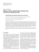
Bạn đang xem bản rút gọn của tài liệu. Xem và tải ngay bản đầy đủ của tài liệu tại đây (2.66 MB, 13 trang )
Hindawi Publishing Corporation
EURASIP Journal on Advances in Signal Processing
Volume 2007, Article ID 57354, 13 pages
doi:10.1155/2007/57354
Research Article
Array Processing and Fast Optimization Algorithms for
Distorted Circular Contour Retrieval
Julien Marot and Salah Bourennane
GSM, Institut Fresnel, CNRS-UMR 6133, Ecole Centrale Marseille, Universit
´
e Aix-Marseille III, D.U. de Saint J
´
er
ˆ
ome,
13397 Marseille Cedex 20, France
Received 19 July 2006; Revised 20 December 2006; Accepted 17 February 2007
Recommended by Wilfried Philips
A specific formalism for virtual signal generation permits to transpose an image processing problem to an array processing prob-
lem. The existing method for straight-line characterization relies on the estimation of orientations and offsets of expected lines.
This estimation is performed thanks to a subspace-based algorithm called subspace-based line detection (SLIDE). In this paper, we
propose to retrieve circular and nearly circular contours in images. We estimate the radius of circles and we extend the estimation
of circles to the retrieval of circular-like distorted contours. For this purpose we develop a new model for virtual signal generation;
we simulate a circular antenna, so that a high-resolution method can be employed for radius estimation. An optimization method
permits to extend circle fitting to the segmentation of objects which have any shape. We evaluate the performances of the proposed
methods, on hand-made and real-world images, and we compare them with generalized Hough transfor m (GHT) and gradient
vector flow (GVF).
Copyright © 2007 J. Marot and S. Bourennane. This is an open access article distributed under the Creative Commons Attribution
License, which permits unrestricted use, distribution, and reproduction in any medium, provided the original work is properly
cited.
1. INTRODUCTION
Circular features in digital images are sought very often in
digital image processing. An image containing one or several
contours is composed of black pixels with value “1” which
represent the contours, over a white background with pixel
value “0.” Circle fitting, in particular, is faced in several appli-
cation fields such as quality inspection for food industry and
mechanical parts, fitting par ticle trajectories [1, 2]. Circle fit-
ting also has applications in microwave engineering, and ball
detection in robotic vision systems [3]. Se veral methods have
been proposed for solving this problem using, among others,
the generalized Hough transform (GHT) [4, 5], array pro-
cessing methods [6, 7], contour-based snakes methods [8, 9].
The formalism proposed by Aghajan [6]permitstodetect
circular or elliptic contours. The coordinates of the center of
a circle are estimated by an array processing method [6] that
works on virtual sig nals generated from the image. Each row
or column of the image is associated with a sensor of a linear
antenna.
In this paper, we propose a new approach which employs
a circular antenna for the estimation of the radius of a circle,
and we propose to adapt an optimization method to retrie ve
the distortions between any nearly-circular contour and a
circle. We adopted a similar strategy in [10], in the case of
the retrieval of approximately rectilinear distorted contours,
by means of a uniform linear antenna.
We choose to employ either the fixed step gradient
method or DIRECT [11] combined with spline interpolation
as an optimization method for the retrieval of the distortions
between the expected distorted contour and a circle that is a
rough approximation of this contour.
The rest of the paper is organized as follows: in Section 2 ,
we set the problem of circle retrieval and show how to model
a circular antenna. In Section 3, we explain why signal gen-
eration out of an image containing circles permits to obtain
linear phase signals when the proposed circular antenna is
used. By using a Minimum Description Length (MDL) crite-
rion, we retrieve the number of concentric circles; then with
a high-resolution method, we estimate the radius of the ex-
pected circles. In Section 4, we derive the numerical com-
plexity of our method and compare it with the complexity
of GHT. In Section 5, we propose to extend the work con-
cerning circular contours to any circular-like contour. In or-
der to adapt the optimization methods proposed in [10, 12],
we simulate the generation of signals from the image on a
2 EURASIP Journal on Advances in Signal Processing
circular antenna with a constant propagation parameter. In
Section 6 we present the results obtained by all proposed
methods through an application to hand-made and real-
world images. We compare the performances of the proposed
methods to those of GHT [5]andGVF[8].
2. PROBLEM SETTING AND VIRTUAL
SIGNAL GENERATION
Our purpose is to estimate the radius of a circle, and the dis-
tortions between a closed contour and a circle that fits this
contour. We propose to employ a circular antenna that per-
mits a particular sig nal generation.
2.1. Problem setting
Figure 1(a) presents a binary digital image I.Anobjectin
the image is made of edge pixels with value “1,” over a
background of zero-valued pixels. The object is close to a
circle with radius value r and center coordinates (l
c
, m
c
).
Figure 1(b) shows a subimage extracted from the original im-
age, such that its top left corner is the center of the circle. We
associate this subimage with a set of polar coordinates (ρ, θ),
such that each pixel of the expected contour in the subimage
is characterized by the coordinates (r + Δρ, θ), where Δρ is
the shift between the pixel of the contour and the pixel of the
circle that roughly approximates the contour and which has
the same coordinate θ. We seek for star-shaped contours, that
is, contours that can be described by the relation ρ
= f (θ),
where f is any function that maps [0, 2π]to
R
+
. The point
with coordinate ρ
= 0 corresponds then to the center of grav-
ity of the contour. For instance to the center in the case of a
circle. A classical method of finding the parameters of circles
is the generalized Hough transform (GHT) [4]. More details
about a fast version of GHT are available in [5]. We apply
rr+ Δρ
l
c
m
c
(a)
θ
r + Δρ
(b)
Figure 1: (a) An image containing a contour close to a circle with
center coordinates (l
c
, m
c
); (b) bottom right quarter of the contour
and pixel coordinates in the polar system (ρ, θ) having its origin on
the center of the circle. r is the radius of the circle. Δρ is the value
of the shift between a pixel of the contour and the pixel of the circle
having the same coordinate θ. Δρ can be either positive or negative.
the GHT to obtain the radius of concentric circles when their
center is known. Its basic principle is to count the number
of pixels that are located on a circle for all possible radius
values. The estimated radius value corresponds to the maxi-
mum number of pixels. Some faster versions were proposed
[5], which avoid the application of the Laplacian operator on
the whole image and restrict the possible radius values to an
apriori-fixed interval. However, the drawback of GHT is still
its elevated computational load.
Hence, there is a need for a faster procedure for estimat-
ing the radius. In [7], Aghajan and Kailath proposed to re-
place the Hough transform by the SLIDE algorithm for re-
trie ving straight lines. SLIDE relies on faster algorithms, the
so-called high-resolution methods of array processing [7].
Therefore, we expect that such methods lead to faster algo-
rithms for circle detection as well, compared to GHT.
The existing methods that combine array processing with
optimization methods employ a sig nal generation scheme
such that only one unknown parameter of the optimization
problem is contained in one component of the generated sig-
nal. In previous work [10, 12], the optimization method that
is set retrieves the phase shift between a linear phase model
and the phase of a signal which is generated from the image.
The phase shift corresponding to each component of the sig-
nal generated on a linear antenna is proportional to the pixel
shift between an approximately-linear contour made of one
pixel per row or column and an initialization straight con-
tour. The purpose of this paper is to retrieve contours which
are no longer approximately linear but approximately circu-
lar. Contours which are approximately circular are supposed
to be made of more than one pixel per row for some of the
rows and more than one pixel per column for some columns.
Therefore, the principles of signal generation which are rele-
vant for the retrieval of approximately linear contours are no
longer relevant for nearly circular contours.
Section 2.2 shows how to associate one sensor of the an-
tenna with one specific orientation in the image for signal
generation.
2.2. Virtual signal generation
We set an analogy between the estimation of a circular con-
tour in an image and the estimation of a wavefront in array
processing. Our basic idea is to obtain a linear phase signal
from an image containing a contour which is a quarter of
circle. The phase of the signals which are virtually generated
on the antenna is constant or varies linearly as a function of
the index of the sensor.
A quarter of circle with radius r and a circular antenna
are represented on Figure 2. We explain here how to gen-
erate sig nal components along several lines in the image,
corresponding to different values of θ in the polar coordi-
nate system of the subimage. The antenna is associated with
the subimage containing any quarter of the expected con-
tour . It is a quarter of circle centered on the top left corner,
and going through the bottom right corner of the subimage.
Such an antenna is adapted to the subimages containing each
quarter of the expected contour (see Figure 2). In practice,
J. Marot and S. Bourennane 3
Sensor S
Sensor i
Sensor 1
D
i
θ
i
1
r
N
s
Figure 2: A subimage is extracted from the processed image: its
top left corner is the center of the expected circle of radius r.The
subimage is associated with a circular array composed of S sensors.
the extracted subimage is possibly rotated such that its top
left corner is the estimated center. A squared image is ob-
tained by zero-padding. Therefore, the antenna has radius
R
antenna
such that R
antenna
=
√
2 · N
subimage
,whereN
subimage
is the number of rows or columns in the subimage. When
we consider the subimage which includes the right bottom
part of the expected contour, we have the relation N
subimage
=
max(N − l
c
, N − m
c
), where l
c
and m
c
are the vertical and
horizontal coordinates of the center of the expected contour
in a Cartesian set centered on the top left corner of the whole
processed image (see Figure 1). Coordinates l
c
and m
c
are es-
timated by the method proposed in [6], which is based on the
generation of signals on a linear antenna by a variable speed
propagation scheme.
The signal generation scheme on a circular antenna is
such that the directions adopted for signal generation go
from the top left corner of the subimage to the correspond-
ing sensor. If the antenna is composed of S sensors, there are
S signal components. Let us consider D
i
, the line that makes
an angle θ
i
with the vertical axis and goes through the top left
corner of the subimage. The ith component z(i)(i
= 1, , S)
of the signal z generated out of the image is given by
z(i)
=
l,m=N
subimage
l,m=1
(l,m)
∈D
i
I(l, m)exp
−
jμ
l
2
+ m
2
. (1)
The integer l (resp., m) indexes the lines (resp., the columns)
of the image. Parameter μ is the propagation parameter [13].
Each sensor indexed by i is associated with a line D
i
hav-
ing an orientation θ
i
= ((i − 1) · π/2)/S. The constraint
(l, m)
∈ D
i
, that is, the pixel with coordinates (l, m)be-
longs to the line with orientation θ
i
, is performed in two
steps: let setl be the set of indexes along the vertical axis, setm
the set of indexes along the horizontal axis, if θ
i
is less than
or equal to π/4, set l
= [1 : N
subimage
] and set m =[1 :
N
subimage
] · tan(θ
i
),ifθ
i
is greater than π/4, set m = [1 :
N
subimage
] and set l =[1 : N
subimage
] · tan(π/2 − θ
i
).Sym-
bol
· means integer part. Dividing the generation process
in two steps allows to work with low-valued angles and ob-
tain lower errors when integer parts are computed. The min-
imum number of sensors that permits a perfect characteriza-
tion of any possibly distorted contour is the number of pixels
that would be virtually aligned on a quarter of circle having
radius
√
2 · N
subimage
. Therefore, the minimum number S of
sensors is
√
2 ·N
subimage
. In this equation, the presence of the
term (l, m)
∈ D
i
shows that only the pixels of the image that
are crossed by line D
i
are taken into account for signal gen-
eration. The term I(l, m) indicates that only pixels that have
value different from 0 are taken into account for signal gen-
eration.
3. PROPOSED METHOD FOR RADIUS ESTIMATION
In the most general case, there exists more than one circle
for one center. We show how several possibly-close radius
values can be estimated with a high-resolution method. For
this, we use a variable speed propagation scheme toward cir-
cular antenna. We propose a method for the estimation of
the number d of concentric circles, and the determination
of each radius value. For this purpose, we employ a variable
speed propagation scheme [13]. We set μ
= α(i −1), for each
sensor indexed by i
= 1, , S.From(1), the signal received
on each sensor is
z(i)
=
d
k=1
exp
−
jα( i − 1)r
k
+ n(i), i = 1, , S,(2)
where r
k
, k = 1, , d are the values of the radius of each
circle, and n(i) is a noise term that can appear because of
the presence of outliers. All components z(i) compose the
observation vector z. From the observation vector we build
K vectors of length M with d<M
≤ S − d + 1. Note that
the number of sensors can be chosen relatively low, as soon
as S>d: the linear phase relationship holds whatever the
number of sensors S. In order to maximize the number of
subvectors [10], we choose K
= S +1− M. By grouping all
subvectors in matr ix form, we obtain
Z
K
=
z
1
, , z
K
,(3)
where
z
l
= A
M
s
l
+ n
l
, l = 1, , K. (4)
A
M
= [a(r
1
), , a(r
d
)] is a Vandermonde type matrix of size
M
× d,
a
r
k
=
1, exp
− jαr
k
,exp
− jα2r
k
, ,
exp
− jα(S − 1)r
k
T
(5)
T denotes transpose, s
l
= [1, 1, ,1]
T
is a length d vector
with all values equal to one.
The signal model of ( 4) suits the frequency estimation
method Estimation of Parameters by Rotational Invariance
Techniques (ESPRIT) proposed in [14] and TLS-ESPRIT, a
Total Least Squares version of ESPRIT. We choose to em-
ploy the subspace-based method TLS-ESPRIT, which has ex-
hibited a good behavior in the application of array process-
ing to straight line detection [15]. TLS-ESPRIT works on
4 EURASIP Journal on Advances in Signal Processing
the measurements obtained from two overlapping subarrays,
and falls into two parts: the estimation of a covariance ma-
trix and the application of a total least squares criterion. The
estimated radius values are obtained in the same way as the
orientation of straight lines are obtained in [13]:
r
k
=
1
α
Im
ln
λ
k
λ
k
, k = 1, , d,(6)
where Im denotes imaginary part,
{λ
k
, k = 1, , d} are the
eigenvalues of a diagonal unitary matrix that relates the mea-
surements from the first subarray to the measurements re-
sulting from the second subarray. At this point, any circle is
characterized by its center coordinates and its radius.
4. NUMERICAL COMPLEXITY OF THE METHODS
In the general case, the image contains outlier pixels and sev-
eral concentric circles. First, as concerns the estimation of the
coordinates of the center [6]: it is performed by signal gen-
eration upon a linear antenna located on one horizontal and
then one vertical side of the image, followed by TLS-ESPRIT
method. This antenna contains N-sensors, each correspond-
ing to one row or column. The estimation of the coordinate
of the center requires the following operations and computa-
tional complexity, for each coordinate along horizontal and
vertical axes [6]:
(i) variable speed propagation scheme upon a linear an-
tenna aside the image: N
2
operations [7];
(ii) application of TLS-ESPRIT to the covariance matrix of
the generated signals: for the estimation, and respec-
tively the fast eigendecomposition, of the covariance
matrix in TLS-ESPRIT method [13, 16]: N
· M, and,
respectively, M
2
.
We ch oose M
=
√
N, as recommended in [13]. The com-
putational complexity for center retrieval is then N
2
+ N ·
(
√
N +1).
As concerns the estimation of the radius values, we re-
mind that d is the number of concentric circles and the di-
mension of the signal subspace in the covariance matrix in
TLS-ESPRIT method. The computational complexity of the
steps of our method for radius estimation is
(i) for signal generation [7, 16]: the number of sensors
multiplied by the number of pixels that are crossed by
each line D
i
, that is, S · N
subimage
or equivalently S · N;
(ii) for the estimation, and, respectively, the fast eigende-
composition, of the covariance matrix in TLS-ESPRIT
method [13, 16]: S
· M, and, respectively, d · M
2
.
We choo se M
=
√
S, as recommended in [13]. The compu-
tational complexity of the angle estimation method is then
S
· N + S · (
√
S + d). In practice, the order of magnitude of
S is N, and the computational load of the proposed method
for center and radius estimation is N
2
.
As concerns the generalized Hough transform, we dis-
cretize the ρ axis to the minimum required number of val-
ues, that is,
√
2 · N for the computation of the accumulator.
Also, the θ axis for counting the edge pixels is discretized to
√
2·N values (
√
2·N is the minimum number of orientations
that permits to characterize any contour in the image, see
Section 2.2). In these conditions, the order of magnitude of
the computational load of the generalized Hough transform,
for the estimation of the center and the radius of the circles,
is N
3
[5]. To conclude, the computational complexity of the
proposed method is N
2
,ascomparedtoN
3
for the gener-
alized Hough transform. The same order of magnitude of
computational loads was obtained in [7] when SLIDE algo-
rithm was compared with the Hough transform for straight
line retrieval.
5. OPTIMIZATION METHOD FOR THE ESTIMATION OF
NEARLY CIRCULAR CONTOURS
The optimization methods proposed in [10, 12] assume that
one component of the generated signal is associated with
only one unknown for the optimization method, namely
the pixel shift between the initialization contour and the ex-
pected contour at one row (or column) of the image. We pro-
pose to employ a circular antenna and to retrieve the shift
values between an initialization circle and the expected con-
tour, along several directions in the image. These directions
go through the center of the initialization circle and have sev-
eral orientations.
We work successively on each quarter of circle, and re-
trieve the distortions between one quarter of the initializa-
tion circle and the part of the expected contour that is lo-
cated in the same quarter of the image. As an example, in
Figure 1, the right bottom quarter of the considered image is
represented in Figure 1(b). Here is an optimization strategy
inspired by [10]: a contour in the considered subimage can
be described in a set of polar coordinates by
{ρ(i), θ(i), i =
1, , S}. We aim at estimating the S unknowns ρ(i),
i
= 1, , S that chara cterize the contour, forming a vector
ρ
=
ρ(1), ρ(2), , ρ(S)
T
. (7)
The basic idea is to consider that ρ canbeexpressedas
ρ
= [r +Δρ(1), r+Δρ(2), , r+Δρ(S)]
T
(see Figure 1), where
r is the radius of a circle that approximates the expected con-
tour. The optimization method that we employ aims at esti-
mating
{Δρ(i), i = 1, , S}, that is, the shifts between the
initialization circle and the expected contour.
By making an analogy with (2) and keeping a constant
propagation parameter, the components of signal z gener-
ated out of the image containing the expected contour are
the following:
z(i)
= exp
−
jμρ(i)
, ∀i = 1, , S. (8)
Equation (8) is obtained from (2) by replacing one constant
r
k
by a radial coordinate ρ(i), that can be different for each
sensor i. So we try to recreate the signal defined in (8)from
whichweignoretheS parameters. We start from an initial-
ization vector ρ
0
, characterizing a quarter of circle that ap-
proximates the expected distorted contour in the considered
subimage. The S components of ρ
0
are equal to r, the radius
value that was previously estimated ρ
0
= [r, r, , r]
T
.Then,
J. Marot and S. Bourennane 5
with k indexing the steps of this recursive algorithm, we min-
imize
J
ρ
k
=
z − z
estimated for ρ
k
2
,(9)
where
·represents the norm induced by the usual scalar
product of
C
S
. The components of z
estimated for ρ
k
are defined
in the same way as the components of z as a function of
the components of ρ
k
, and the components of ρ
k
are ob-
tained from the components of ρ
0
by adding a shift ρ
k
=
[r + Δρ
k
(1), r + Δρ
k
(2), , r + Δρ
k
(S)]
T
. In this paper, we
use the fixed step gradient method. The variable step gradi-
ent method could also be used. The vectors of the series are
obtained by the relation
∀k ∈ N : ρ
k+1
= ρ
k
− λ∇
J
ρ
k
, (10)
where 0 <λ<1 is the step for the descent. The recurrence
loop is
ρ
k
−→ z
estimated for ρ
k
−→ J
ρ
k
. (11)
The gradient is estimated using finite differenc es. When k
tends to infinity, the criterion J tends to zero and ρ
k
(i) =
r + Δρ(i) = ρ(i), for all i = 1, , S.
We denote by
ρ the vector containing all estimated val-
ues ρ
k
(i), i = 1, , S,withk tending to infinity. A more
elaborated method based on DIRECT algorithm and spline
interpolation can be adopted in order to reach the global
minimum of the criterion J of (9) to be minimized. This
method is applied to modify recursively signal z
estimated for ρ
k
;
at each step of the recursive procedure vector ρ
k
is computed
by making an interpolation between some “node” values that
are retrie ved by DIRECT.
The interest of the combination of DIRECT with spline
interpolation comes from the elevated computational load
of DIRECT. Details about DIRECT algorithm are available
in [11]. Its main property is that it is a global optimiza-
tion method it permits to obtain the global minimum of a
function. DIRECT normalizes the research space in a hy-
percube and evaluates the solution which is located in the
center of this hypercube. Then, some solutions are evaluated
and the hypercube is divided into smaller cubes supporting
the zones were the evaluations are small. Let O be an inte-
ger lower than S. A cubic spline f interpolating on the par-
tition y(1), , y(O) that we call “node points,” to the ele-
ments ρ(1), , ρ(S), is a function for which f (y(k))
= ρ(k)
for k
= 1, , O. It is a piecewise polynomial function that
consists of O
− 1 cubic polynomials f
k
defined on the ranges
[y(k), y(k + 1)]. Furthermore, each f
k
is joined at y(k), for
k
= 2, , O − 1, such that ρ
(k) = f
(y(k)) and ρ
(k) =
f
(y(k)) are continuous. The kth polynomial curve, f
k
,is
defined over the fixed interval [y(k), y(k + 1)] and is a third-
order polynomial. Then interpolation provides an approxi-
mate value of S elements starting from O<Selements.
Spline interpolation permits to obtain a continuous esti-
mated contour and cubic splines provide a good compromise
between computational load and accuracy of the interpola-
tion.
The computational load of DIRECT algorithm grows
rapidly when the number of sensors, or equivalently the
number of unknown phase values, increases. We accelerate
DIRECT algorithm by reducing the number of retrieved un-
knowns and then we propose spline interpolation to obtain
the S components of
ρ; we interpolate a subset of values of
ρ
k
, which are retrieved by DIRECT algorithm. The more the
interpolation nodes are, the more precise the estimation be-
comes, but the slower the algorithm becomes.
6. RESULTS OBTAINED BY THE PROPOSED METHODS
We apply here the proposed methods to hand-made and real-
world images. First we compare our methods based on sig-
nal generation upon a circular antenna with the generalized
Hough transform (GHT). Secondly we compare our meth-
ods with gradient vector flow (GVF) when images with dis-
torted contours are considered. The efficiency of the pro-
posed methods is measured from the final result thanks to the
criterion ME
ρ
, which is the mean error over the estimation
of coordinates of the pixels of the curve. For the four quar-
ters of an image, the coordinates of the pixels of the curve are
contained in vector ρ defined in (7), and their estimates are
contained in vector
ρ. ME
ρ
is defined by
ME
ρ
=
1
S
S
i=1
ρ(i) − ρ(i)
, (12)
where
|·|stands for absolute value. The error over all pix-
els of the contour is the mean of the error obtained with each
quarter of image. When several contours are retrieved for one
image, the mean value of the error over all contours is pro-
vided.
6.1. Circle retrieval
The proposed method for circle fitting is applied to hand-
made and real-world images having N
= 200 columns and
rows.WeadoptanumberofsensorsS
= 400 for each quar-
ter of image, which is larger than the minimum acceptable
value. Procedures for center and radius estimation are run
with propagation parameter α
= 1.35 · 10
−2
. When TLS-
ESPRIT method is run the length of each subarray, as rec-
ommended in [13], M
=
√
S = 20. The s ignal generation
scheme dedicated to distortion estimation is run with con-
stant propagation speed μ
= 5·10
−3
. This value avoids phase
indetermination [12].
6.1.1. Nonnoisy image: computational times
We first considered the case of an image containing two con-
centric circles. Thanks to the adopted formalism, this prob-
lem is equivalent to the resolving of two close-valued fre-
quencies in array processing. High-resolution methods were
specifically created to face this problem and exhibited a very
good behavior [14]. In this case, starting from the signals
generated on the circular antenna, MDL criterion permits
to estimate the number of expected circles, and the high-
resolution method TLS-ESPRIT manages to estimate the
6 EURASIP Journal on Advances in Signal Processing
20 40 60 80 100 120 140 160 180 200
200
180
160
140
120
100
80
60
40
20
(a)
20 40 60 80 100 120 140 160 180 200
200
180
160
140
120
100
80
60
40
20
(b)
Figure 3: Center and radius estimation, two circles: (a) processed, (b) result (superimposed), with the proposed method for radius estima-
tion or equivalently with GHT: ME
ρ
= 0.1(resp.,0.3forGHT).
radius of each circle. The expected radius values are 85 and
90 pixels (see Figure 3(a))thus,differing by only 6%. The es-
timated radius values obtained with the proposed method
are 85.1 and 89.9 pixels, and the required computational time
is 0.359 seconds, on a 3.0 GHz Pentium 4 PC running Win-
dows. The same processor and the same software are used
throughout a ll experiments. The slight bias may come from
the signal generation process. When GHT is applied to ob-
tain an estimation of the radius values, ρ and θ parameters
are b oth quantized to S values to create the accumulator. Esti-
mated radius values are 84.7 and 90.3 pixels, and the required
computational time is 2.2 seconds. Visually, there is no differ-
ence between the results of both methods (see Figure 3(b)).
6.1.2. Noisy images: statistical results
We now consider the case of a noisy image. High-resolution
methods are known to cope with noisy signals. In particular,
TLS-ESPRIT method works optimally in the case of uncorre-
lated white noise [14]. This condition holds for signals gen-
erated out of an image by a propagation scheme, they are im-
paired by an uncorrelated white Gaussian noise if the noisy
pixels are randomly distributed in the image [7]. This per-
mits to predict that TLS-ESPRIT method should work opti-
mally with this kind of noisy image. We performed a statisti-
cal study (1000 trials) in order to compare the robustness of
the proposed method a nd the generalized Hough transform,
for radius estimation. In order to impair our hand-made im-
ages, we add 20% of Gaussian noise with mean 0.02 and
standard deviation 0.009. Figure 4 shows an example of pro-
cessed image containing a circle with r adius value r, and the
result obtained with the proposed method (see Figure 4(a)),
and an example of processed image and the result obtained
with GHT (see Figure 4(b)). Mean error ME
r
over the radius
value is defined by ME
r
= (1/1000)(
1000
j
=1
|r − r
j
|), where j
indexes the trials and
r
j
is the radius estimation obtained at
the jth trial. The second criterion is the root mean square er-
ror RMSE
r
,definedbyRMSE
r
=
(1/1000)
1000
j
=1
(r
j
− r)
2
.
50 100 150 200 50 100 150 200
200
180
160
140
120
100
80
60
40
20
200
180
160
140
120
100
80
60
40
20
(a)
50 100 150 200 50 100 150 200
200
180
160
140
120
100
80
60
40
20
200
180
160
140
120
100
80
60
40
20
(b)
Figure 4: One circle: radius estimation by the proposed method
and GHT: (a) processed image and result with our method, (b) pro-
cessed image and result with GHT.
J. Marot and S. Bourennane 7
0
2
46 8
Noise (%)
0
0.1
0.2
0.3
0.4
0.5
0.6
0.7
0.8
0.9
1
ME
GHT
Proposed method
0
2
468
Noise (%)
0
0.005
0.01
0.015
0.02
0.025
0.03
0.035
0.04
RMSE
GHT
Proposed method
Figure 5: Mean value (pixels) and root mean square error (pixels)
of the mean bias over the radius value, as a function of the percent-
age of noisy pixels.
The results presented in Figure 5 show that ME
r
values differ
by less than 0.1 pixel and are always less than 1 pixel. RMSE
r
values differ by less than 0.05 pixel. Therefore, statistical re-
sults obtained with both methods are very close, slightly bet-
ter for the GHT, at the expense of a larger computational
time.
6.1.3. Circle fitting: real-world images
Proposed methods can be applied to practical issues. We as-
sume that all expected contours are centered on the middle
of the image. We first give the result obtained by circle fitting
(see Figure 6).
Figure 6 shows that the contour of each object presented
is efficiently retrieved.
6.1.4. Ellipse fitting and limitations
An ellipse is no longer characterized by a constant radius, but
by two axial parameters which are the largest and the small-
est distances between the contour and its center. In the case
where an ellipse is expected, the signal model proposed in (2)
does not hold because one cannot define one constant fre-
quency in the generated signal, as it was done in the case of
a circle. However, when we perform the eigendecomposition
of the covariance matrix of the recorded signal snapshots, we
note that there exist two dominant eigenvalues. Therefore,
the dimension of the signal subspace is fixed to two. Equation
(6) leads to the two approximate values of the axial param-
eters of the ellipse. Then the proposed optimization method
cancels the shift between the initialization ellipse and the ex-
pected contour. As a comparison, we expose the result ob-
tained with the method proposed in [6] that leads to the ax-
ial parameters of the ellipse through signal generation upon
a linear antenna. Figure 7 shows the results obtained from
an image containing a slightly distorted ellipse, with axial
parameters 65 and 75 pixels. The estimated values provided
by the method proposed in [6] are 65.6 and 65.6 pixels (see
Figure 7(b)). The bias on one axial parameter can be due to
the presence of a slight distortion. The estimation provided
by the GHT, which aims at retrieving only one radius pa-
rameter, is 65.7 pixels (see Figure 7(c)). The estimated val-
ues provided by our method are 67.0 and 78.6 pixels (see
Figure 7(d)). The slight bias on these values can come from
the distortion of the ellipse. This bias is lower than in the
case of Figure 7(b); when the circular antenna is used, all sen-
sors receive a nonzero signal component and then all com-
ponents contribute in the estimation of the expected param-
eters. This permits to our circular antenna to cope more ef-
ficiently with slight distortions than when a linear antenna is
used. When our method for retrieval of the distortions is run
with 3000 iterations of gradient, with descent step parame-
ter λ
= 0.02, the bias between initialization contour and ex-
pected contour is canceled (see Figures 7(e) and 7(f)). Then
our method based on a circular antenna copes with the harsh
case of a slightly distorted ellipse, for this we choose cor-
rectly the dimension of the signal subspace obtained from the
generated signal. We consider now the case of an ellipse for
which the ratio between axial parameters is far from unity.
Figure 8 shows the results obtained from an image contain-
ing an ellipse with axial parameters 45 and 85 pixels. The es-
timated values provided by the method proposed in [6]are
47.3 and 88.6 pixels (see Figure 8(b)). The estimation pro-
vided by the GHT, which aims at retrieving only one radius
parameter, is 45 pixels (see Figure 8(c)). The estimated val-
ues provided by our method are 49.7 and 96.8 pixels (see
Figure 8(d)). The bias on these values can come from a signal
model which is not adequate. Then our method based on a
circular antenna copes with the case of an ellipse whose axial
parameters are close to each other but is limited as soon as
the ratio between axial parameters is far from unity. This is
due to the assumption of linear phase in the signal generated
on the circular antenna (see (2)). In the next subsection we
will focus on distorted circles.
6.2. Distorted contours
In this subsection we illustrate the performances of the opti-
mization methods proposed for the estimation of the distor-
tions between an initialization circle and the expected con-
tour. We compare the abilities of our methods with the abil-
ities of GVF. g radient algorithm, which is less robust but
faster than DIRECT combined with spline interpolation, is
employed for hand-made images. Descent step parameter is
λ
= 0.02, and 3000 iterations are necessary.
6.2.1. Illustration of the results obtained with gradient
algorithm: hand-made images
The result obtained in Figure 9 shows that even if there ex-
ists a bias between real and estimated values of the radius,
8 EURASIP Journal on Advances in Signal Processing
20 40 60 80 100 120 140 160 180 200
200
180
160
140
120
100
80
60
40
20
20 40 60 80 100 120 140 160 180 200
200
180
160
140
120
100
80
60
40
20
(a)
20 40 60 80 100 120 140 160 180 200
200
180
160
140
120
100
80
60
40
20
20 40 60 80 100 120 140 160 180 200
200
180
160
140
120
100
80
60
40
20
(b)
Figure 6: (a) Processed image, (b) result obtained with the proposed method for radius estimation. ME
ρ
= 0.4 and 0.6 pixel.
20 40 60 80 100 120 140 160 180 200
200
180
160
140
120
100
80
60
40
20
(a)
20 40 60 80 100 120 140 160 180 200
200
180
160
140
120
100
80
60
40
20
(b)
20 40 60 80 100 120 140 160 180 200
200
180
160
140
120
100
80
60
40
20
(c)
20 40 60 80 100 120 140 160 180 200
200
180
160
140
120
100
80
60
40
20
(d)
20 40 60 80 100 120 140 160 180 200
200
180
160
140
120
100
80
60
40
20
(e)
20 40 60 80 100 120 140 160 180 200
200
180
160
140
120
100
80
60
40
20
(f)
Figure 7: Ellipse fitting: (a) processed. (b) Difference processed and result by the existing method for ellipse retrieval [6]. (c) Difference
processed and result by the GHT. (d) Difference processed and result obtained after applying the proposed method: ME
ρ
= 2.8 pixel. (e)
Difference processed and result obtained after applying gradient method: ME
ρ
= 0.7 pixel. (f) Superposition processed and result obtained
after applying gradient method.
J. Marot and S. Bourennane 9
20 40 60 80 100 120 140 160 180 200
200
180
160
140
120
100
80
60
40
20
(a)
20 40 60 80 100 120 140 160 180 200
200
180
160
140
120
100
80
60
40
20
(b)
20 40 60 80 100 120 140 160 180 200
200
180
160
140
120
100
80
60
40
20
(c)
20 40 60 80 100 120 140 160 180 200
200
180
160
140
120
100
80
60
40
20
(d)
Figure 8: Ellipse fitting: (a) processed. (b) Difference processed and result by the existing method for ellipse retrieval [6]. (c) Difference
processed and result by the GHT. (d) Difference processed and result obtained after applying the proposed method.
the optimization method finds the expected circle. The case
of Figure 9 is not handled easily by GVF which has to be ini-
tialized close to the expected contour to converge in the same
computational time as gradient.
We now consider the case of a noisy image. A least-
squares criterion gives an optimal result in the case of Gaus-
sian noise. Then, as the proposed optimization methods are
applied to minimize a least-squares criterion over the gen-
erated signal (see (9)), the result obtained should be opti-
mal. We consider then a noisy image containing a slightly
distorted circle. In order to impair our hand-made images,
we add a Gaussian noise to a percentage p of the pixels of
the nonnoisy image. We adopt the same parameters as in
Section 6.1.2. The image considered in Figure 10 is impaired
by p
= 20% of noisy pixels.
We also give the result obtained with GVF, from the same
image, the same initialization contour and another noise re-
alization with the same parameters. Indeed, there exists only
one continuous contour to be retrieved and the initialization
circle is close to the expected contour, which leads to a com-
putational time which is the same as when the gradient op-
timization method is u sed. We choose the follow ing param-
eters, that lead to a good result in terms of mean error and
requires an acceptable computational time: parameter values
are [8] α
GVF
= 0.5 (tension, rather elevated because of the
presence of noise), β
GVF
= 0.01 (rigidity), γ
GVF
= 1 (regu-
larization coefficient), κ
GVF
= 0.8 (Gradient strength coef-
ficient), μ
GVF
= 0.15 (regularization parameter in the GVF
formulation), and 120 iterations are asked for the deforma-
tion.
Gradient method cancels the pixel shifts between the ini-
tialization circle and the expected circle. GVF method also
cancels the pixel shifts. Computational (CPU) times which
are needed for center estimation and radius estimation are,
respectively, 3.8
·10
−2
seconds and 7.8 ·10
−1
seconds. Signal
generation lasts 0.14 seconds and fixed step gradient method
lasts 1.9 seconds each time they are run. Thus 8.2 seconds
are needed for the four quarters of image. Running GVF
method lasts 9.1 seconds. We tested the variable step gradient
method, which gives the same visual result and is ten times
faster than the fixed step gradient method for this example.
However, we will use fixed step gradient in the following. In
this way, the performances of gradient and GVF in terms of
mean error are evaluated for computational times that differ
by only 10%.
6.2.2. Statistical results obtained with gradient algorithm
applied to noisy hand-made images
Fixed step gradient method and GVF [8] are applied to im-
ages containing a slightly-distorted circle. We adopt the same
noise parameters as in Section 6.1.2, considering various
10 EURASIP Journal on Advances in Signal Processing
20 40 60 80 100 120 140 160 180 200
200
180
160
140
120
100
80
60
40
20
(a)
20 40 60 80 100 120 140 160 180 200
200
180
160
140
120
100
80
60
40
20
(b)
20 40 60 80 100 120 140 160 180 200
200
180
160
140
120
100
80
60
40
20
(c)
Figure 9: One circle: biased radius estimation, and application of
gradient algorithm: (a) processed. (b) Initialization. (c) Superposi-
tion processed and result obtained after applying gradient method:
ME
ρ
= 0.15 pixel.
noise percentage values. All these images are similar to the
processed image of Figure 10. In order to evaluate only the
performances of the proposed optimization method and
GVF, both methods are initialized assuming the apriori
knowledge of the center and the radius of the distorted cir-
cle. The parameters of signal generation and signal process-
ing methods, for the proposed optimization method, are
the same as in Section 6.1. Statistical results presented be-
low are obtained with 15 images, each containing a differ-
ent distorted circle. Noise parameters are the same as those
employed for the study of r adius estimation, propagation
parameter is μ
= 5 · 10
−3
. 1000 iterations are necessary
for gradient algorithm. Computational times are respectively
4.5 seconds for gradient algorithm on each quarter of im-
age and 17 seconds for GVF method. So performances are
compared for the same computational time. GVF method is
run w ith the same parameter values as in Section 6.1.The
first criterion that is employed to measure the accuracy of
the results is the mean value of ME
ρ
.MeanerrorME is de-
fined by ME
= (1/1500)
15
i
=1
(
100
j
=1
ME
ρ
i
j
), where j indexes
the trials and ME
ρ
i
j
is the mean error over all pixels of the
contour obtained at the jth trial for the ith image. The sec-
ond criterion is the root mean square error RMSE, defined
by RMSE
=
(1/1500)
15
i=1
100
j=1
(ME
ρ
i
j
)
2
.Therightim-
age of Figure 11 shows that mean error values are less than
one pixel for each noise percentage value and for both meth-
ods, thus, acceptable for many applications. The error values
obtained with GVF method are between 11 and 27% higher
for the considered values of noise percentage. The low-root
mean square error values show that both methods are ro-
bust to noise impairment. The left image of Figure 11 shows
that the root mean square error values obtained with GVF
are between 28 and 41% higher than the values obtained with
the proposed method. The errors obtained with the proposed
method are not due to the optimization method, w hich leads
to a value zero for the criterion to be optimized. Errors come
from the signal generation process: for noisy images the gen-
erated signal is corr upted and its phase exhibits unexpected
fluctuations. The errors obtained with GVF come from a
nonoptimal interplay between all parameters for all images.
6.2.3. Distorted circle fitting: real-world images
The parameters of signal generation and signal processing
methods for radius estimation are the same as in Section 6.1.
We assume that all expected contours are centered on the
middle of the image. Real-world images are supposed to be
harsher to process than hand-made images because of the
presence of random noise and disruptions in the expected
contours. Gradient algorithm would obligatorily focus on
noise pixels in the disrupted sections of the expected con-
tour. That is why we use the combination of the robust DI-
RECT method and spline interpolation which reduces the
computational time of DIRECT and leads to a continuous re-
sult contour. Figure 12 gives the result obtained by gradient
method and DIRECT combined with spline interpolation
on the first real-world image, that concerns the practical is-
sue of calibrating pies. DIRECT combined with spline is fast
enough if a small number of nodes are chosen for the inter-
polation to be compared to the GVF method. Therefore, we
also give the result obtained by GVF. Figure 12(a) gives the
original color image. Figure 12(b) gives the initialization cir-
cle superimposed to the processed image. Figure 12(c) shows
that gradient provides us with a contour which is not con-
tinuous and whose pixels go aside the pixels of the expected
contour. When gradient method is employed, the mean er-
ror value ME
ρ
is 1.7 pixel. Parameters used to run gradient
J. Marot and S. Bourennane 11
20 40 60 80 100 120 140 160 180 200
200
180
160
140
120
100
80
60
40
20
(a)
20 40 60 80 100 120 140 160 180 200
200
180
160
140
120
100
80
60
40
20
(b)
20 40 60 80 100 120 140 160 180 200
200
180
160
140
120
100
80
60
40
20
(c)
20 40 60 80 100 120 140 160 180 200
200
180
160
140
120
100
80
60
40
20
(d)
Figure 10: (a) Processed. (b) Initialization by the existing method for center estimation [6] and the proposed method for radius estimation.
(c) Superposition processed and result obtained after applying gradient method: ME
ρ
= 0.55 pixel. (d) Superposition processed and result
obtained after apply ing GVF method [8]: ME
ρ
= 0.75 pixel.
02468
Noise (%)
0.75
0.8
0.85
0.9
0.95
1
ME
GVF method
Proposed method
0
2
468
Noise (%)
0.075
0.08
0.085
0.09
0.095
0.1
0.105
0.11
0.115
RMSE
GVF method
Proposed method
Figure 11: Mean value (pixels) and root mean square error (pixels),
as a function of the percentage of noisy pixels, of the mean pixel bias
value over the circle.
method are the same as the parameters used in Section 6.1.
Figure 12(d) gives the result obtained with GVF, run with the
same parameters as in Section 6.2.2.MeanerrorvalueME
ρ
is 1.9 pixel. With this method, the result obtained is continu-
ous and exhibits low-curvature variations, but the numerous
noise pixels prevent the active contour from converging ex-
actly toward the expected contour.
Figure 12(e) gives the result obtained by DIRECT com-
bined with spline interpolation. When this robust optimiza-
tion method is used, the mean error value ME
ρ
is 1.6 pixel.
Parameters used for running DIRECT and spline interpola-
tion are the following: 6 interpolation nodes, and 5 iterations
for DIRECT. Computational times are, respectively, 30 and
40 seconds for GVF and the proposed method.
7. CONCLUSION
We have shown in this paper how array processing and op-
timization methods can be applied to estimate distorted cir-
cular contours in images. In particular, we have shown the
interest of the use of a circular antenna for the generation
of linear phase signals when the processed image contains
a circular contour. This facilitates the application of high-
resolution methods and optimization algorithms in the esti-
mation of distorted circles in images. We proposed a method
for the estimation of several possibly close radius values, and
adapted an optimization strategy to the case of the retrieval
12 EURASIP Journal on Advances in Signal Processing
20 40 60 80 100 120 140 160 180 200
200
180
160
140
120
100
80
60
40
20
(a)
20 40 60 80 100 120 140 160 180 200
200
180
160
140
120
100
80
60
40
20
(b)
20 40 60 80 100 120 140 160 180 200
200
180
160
140
120
100
80
60
40
20
(c)
20 40 60 80 100 120 140 160 180 200
200
180
160
140
120
100
80
60
40
20
(d)
20 40 60 80 100 120 140 160 180 200
200
180
160
140
120
100
80
60
40
20
(e)
Figure 12: (a) Processed image. (b) Initialization. (c) Result obtained with gradient method. (d) Result obtained with GVF. (e) Result
obtained with DIRECT combined with spline interpolation.
of distorted circles. The proposed method for radius esti-
mation is faster than the generalized Hough transform and
exhibits a good statistical behavior. This also holds for our
optimization methods that we compared with GVF. We ap-
plied the robust optimization method based on DIRECT and
spline interpolation to real-world images coming from prac-
tical issues. Real-world images were processed successfully,
low pixel bias are obtained compared with the other consid-
ered methods. Further work could consist in estimating the
parameters of multiple circles with different radius and also
different center.
ACKNOWLEDGMENT
The authors would like to thank the anonymous reviewers
who contributed to the quality of this paper by providing
helpful suggestions.
REFERENCES
[1] J. F. Crawford, “A noniterative method for fitting circular
arcs to measured points,” Nuclear Instruments and Methods in
Physics Research, vol. 211, no. 2, pp. 223–225, 1983.
[2] V. Karim
¨
aki, “Effective circle fitting for particle trajectories,”
Nuclear Instruments and Methods in Physics Research Section
A, vol. 305, no. 1, pp. 187–191, 1991.
[3] G. Coath and P. Musumeci, “Adaptive arc fitting for ball detec-
tion in robocup,” in Proceedings of APRS Workshop on Digital
Image Computing (WDIC ’03), pp. 63–68, Brisbane, Australia,
February 2003.
[4]D.H.Ballard,“GeneralizingtheHoughtransformtodetect
arbitrary shapes,” Pattern Recognition, vol. 13, no. 2, pp. 111–
122, 1981.
[5] C.L.Tisse,L.Martin,L.Torres,andM.Robert,“Personiden-
tification technique using human iris recognition,” in Inter-
national Conference on Vision Interface (VI ’02), pp. 294–299,
Calgar y, Canada, May 2002.
[6] H. K. Aghajan, “Subspace techniques for image understanding
and computer vision,” Ph.D. dissertation, Stanford University,
Stanford, Calif, USA, 1995.
[7] H. K. Aghajan and T. Kailath, “Sensor array processing tech-
niques for super resolution multi-line-fitting and straight edge
detection,” IEEE Transactions on Image Processing, vol. 2, no. 4,
pp. 454–465, 1993.
[8] C. Xu and J. L. Prince, “Gradient vector flow: a new external
force for snakes,” in Proceedings of the IEEE Computer Soci-
ety Conference on Computer Vision and Pattern Recognition,pp.
66–71, San Juan, Puerto Rico, USA, June 1997.
[9] X. Xie and M. Mirmehdi, “RAGS: region-aided geometric
snake,” IEEE Transactions on Image Processing, vol. 13, no. 5,
pp. 640–652, 2004.
[10] S. Bourennane and J. Marot, “Contour estimation by array
processing methods,” EURASIP Journal on Applied Signal Pro-
cessing, vol. 2006, Article ID 95634, 15 pages, 2006.
J. Marot and S. Bourennane 13
[11] D. R. Jones, C. D. Perttunen, and B. E. Stuckman, “Lips-
chitzian optimization without the Lipschitz constant,” Jour-
nal of Optimization Theory and Applications,vol.79,no.1,pp.
157–181, 1993.
[12] S. Bourennane and J. Marot, “Optimization and interpolation
for distorted contour estimation,” in Proceedings of IEEE Inter-
national Conference on Acoustics, Speech and Signal Processing
(ICASSP ’06), vol. 2, pp. 717–720, Toulouse, France, May 2006.
[13] H. K. Aghajan and T. Kailath, “SLIDE: subspace-based line de-
tection,” IEEE Transactions on Pattern Analysis and Machine
Intelligence, vol. 16, no. 11, pp. 1057–1073, 1994.
[14] R. Roy and T. Kailath, “ESPRIT-estimation of signal param-
eters via rotational invariance techniques,” IEEE Transactions
on Acoustics, Speech, and Signal Processing,vol.37,no.7,pp.
984–995, 1989.
[15] H. K. Aghajan, B. H. Khalaj, and T. Kailath, “Estimation of
multiple 2-D uniform motions by SLIDE: subspace-based line
detection,” IEEE Transactions on Image Processing, vol. 8, no. 4,
pp. 517–526, 1999.
[16] J. Sheinvald and N. Kiryati, “On the magic of SLIDE,” Machine
Vision and Applications, vol. 9, no. 5-6, pp. 251–261, 1997.
J ulien Marot received the Physics engineer-
ing degree from ENSP Marseille, France,
in 2003 and the Image Processing DEA in
2004. Since December 2004, he works as
Ph.D. s tudent in the multidimensional sig-
nal processing group (GSM), Fresnel Insti-
tute (CNRS UMR-6133). His research inter-
ests include applied image processing and
signal processing.
Salah Bourennane received his Ph.D. de-
gree from Institut National Polytechnique
de Grenoble, France, in signal processing.
Currently, he is Full Professor at the Ecole
Centrale de Marseille, France. His research
interests are in statistical signal processing,
array processing, image processing, multi-
dimensional signal processing, and perfor-
mances analysis.