Báo cáo hóa học: " Research Article Spatial-Temporal Correlation Properties of the 3GPP Spatial Channel Model and the Kronecker MIMO Channel Model" pdf

Hindawi Publishing Corporation
EURASIP Journal on Wireless Communications and Networking
Volume 2007, Article ID 39871, 9 pages
doi:10.1155/2007/39871
Research Article
Spatial-Temporal Correlation Properties of the 3GPP Spatial
Channel Model and the Kronecker MIMO Channel Model
Cheng-Xiang Wang,
1
Xuemin Hong,
1
Hanguang Wu,
2
and Wen Xu
2
1
Joint Research Institute in Signal and Image Processing, School of Engineering and Physical Sciences,
Heriot-Watt University, Edinburgh EH14 4AS, UK
2
Baseband Algorithms and Standardization Laboratory, BenQ Mobile, 81667 Munich, Germany
Received 1 April 2006; Revised 28 November 2006; Accepted 3 December 2006
Recommended by Thushara Abhayapala
The performance of multiple-input multiple-output (MIMO) systems is greatly influenced by the spatial-temporal correlation
properties of the underlying MIMO channels. This paper investigates the spatial-temporal correlation characteristics of the spatial
channel model (SCM) in the Third Generation Partnership Project (3GPP) and the Kronecker-based stochastic model (KBSM) at
three levels, namely, the cluster level, link level, and system level. The KBSM has both the spatial separability and spatial-temporal
separability at all the three levels. The spatial-temporal separability is observed for the SCM only at the system level, but not at the
cluster and link levels. The SCM shows the spatial separability at the link and system levels, but not at the cluster level since its
spatial correlation is related to the joint distribution of the angle of arrival (AoA) and angle of departure (AoD). The KBSM with the
Gaussian-shaped power azimuth spectrum (PAS) is found to fit best the 3GPP SCM in terms of the spatial correlations. Despite
its simplicity and analytical tractability, the KBSM is restricted to model only the average spatial-temporal behavior of MIMO

channels. The SCM provides more insights of the variations of different MIMO channel realizations, but the implementation
complexity is relatively high.
Copyright © 2007 Cheng-Xiang Wang et al. This is an open access article distributed under the Creative Commons Attribution
License, which permits unrestricted use, distribution, and reproduction in any medium, provided the original work is properly
cited.
1. INTRODUCTION
In the 3rd generation (3G) and beyond-3G (B3G) wireless
communication systems, higher data rate transmissions a nd
better quality of services are demanded. This motivates the
investigation towards the full exploitation of time, frequency,
and more recently, space domains. By deploying spatially
separated multiple antenna elements at both ends of the
transmission link, multiple-input multiple-output (MIMO)
technologies can improve the link reliability and provide a
significant increase of the link capacity [1]. It was further
shown in [2] that the MIMO channel capacity grows lin-
early with antenna pairs as long as the environment has suffi-
ciently rich scatterers. To approach the promised theoretical
MIMO channel capacity, practical signal processing schemes
for MIMO systems have been proposed, for example, space-
time processing [3, 4] and space-frequency processing [5].
Both the link capacity and signal processing performance
are greatly affected by fading correlation characteristics of
the underlying MIMO channels [6]. An appropriate char ac-
terization and modeling of MIMO propagation channels are
thus indisp ensable for the development of 3G and B3G sys-
tems. In the literature, MIMO channels are often modeled
by applying a stochastic approach [7, 8]. Stochastic MIMO
channel models can roughly be classified into three types [9],
namely, geometrically-based stochastic models (GBSMs),

Correlation Based Stochastic Models (CBSMs), and Para-
metric Stochastic Models (PSMs). A GBSM is derived from
a predefined stochastic distribution of s catterers by applying
the fundamental laws of reflection, diffraction, and scattering
of electromagnetic waves. The well-known GBSMs are one-
ring [10], two-ring [11], and elliptical [12] MIMO channel
models. CBSMs are another type, in which the spatial corre-
lation properties of a MIMO channel are modeled by statisti-
cal means. A Kronecker-based stochastic model (KBSM) [7],
which is a simplified CBSM, has been adopted as the core
of the link-level MIMO model in the 3rd Generation Part-
nership Project (3GPP) [13]. The third type is PSMs, which
characterize the MIMO channels by using selected param-
eters such as angle of arrival (AoA) and angle of departure
2 EURASIP Journal on Wireless Communications and Networking
(AoD). The received signal is modeled as a super position of
waves, and often adopted into a tapped delay-line structure
for implementation. Within this category, the widely em-
ployed models are the spatial channel model (SCM) [14]for
bandwidths up to 5 MHz and the wideband SCM [15]for
bandwidths above 5 MHz, specified in the 3GPP.
It is important to mention that the above three types of
stochastic MIMO channel models are interrelated. The rela-
tionship between a GBSM and a PSM was theoretically an-
alyzed in [16], while the connection between a GBSM and
a CBSM was demonstrated in [6]. The mapping between a
PSM and a CBSM was addressed only in a few papers [17–
19], where the comparison of the spatial-temporal correla-
tion properties of both types of models was not based on the
same set of parameters. This leaves us a doubt whether the

difference of the spatial-temporal correlation characteristics
is caused by the models’ structural difference or different pa-
rameter generation mechanisms.
The SCM [14] was proposed by the 3GPP for both
link- and system-level simulations, while the KBSM [7]was
mainly used for the link-level MIMO simulations [13]. Both
models have advantages and disadvantages. The SCM can di-
rectly generate channel coefficients, while it does not spec-
ify the spatial-temporal correlation properties explicitly. It is
therefore difficult to connect its simulation results with the
theoretical analyses. Also, the implementation complexity of
the SCM is high since it has to generate many parameters
such as antenna array orientations, mobile directions, delay
spread, angular spread (AS), AoDs, AoAs, and phases. On the
other hand, a KBSM requires less input parameters and pro-
vides elegant and concise analytical expressions for MIMO
channel spatial correlation matrices. This makes the KBSM
easier to be integrated into a theoretical framework. How-
ever, compared with the SCM, KBSMs are often questioned
about the oversimplification of MIMO channel character-
istics. Although both the SCM and KBSM are well known,
some important issues still remain unclear for academia and
industry. These issues include the following question (1)
what is the major physical phenomenon that makes the fun-
damental difference of the two models? (2) under what con-
ditions will the two models exhibit similar spatial-temporal
correlation characteristics? (3) when will we use the SCM or
KBSM as the best tradeoff between the model accuracy and
efficiency? The aim of this paper is to find solutions to the
above unclear questions. For this purpose, we propose to dis-

tinguish the spatial-temporal correlation properties of both
models at three levels, namely, the cluster level, link level, and
system level. Also, the same parameter generator is used for
both models so that the difference of the resulting channel
characteristics is caused only by the fundamental structural
difference between the SCM and KBSM.
The rest of the paper is organized as follows. Section 2
briefly reviews the 3GPP SCM. Its spatial-temporal correla-
tion characteristics are also analyzed. A KBSM and its spatial-
temporal correlation properties a re presented in Section 3.
Section 4 compares the spatial-temporal correlation proper-
ties of the two models. Finally, the conclusions are drawn in
Section 5.
N
N
BS array
MS array
Cluster n
Subpath m
MS direction
of travel
BS array broadside
MS array broadside
Ω
BS
θ
BS
δ
n,AoD
Δ

n,m,AoD
θ
n,m,AoD
Δ
n,m,AoA
θ
n,m,AoA
δ
n,AoA
θ
MS
Ω
MS
θ
v
v
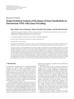
Figure 1: BS and MS angle parameters in the 3GPP SCM with one
cluster of scatterers [14].
2. THE 3GPP SCM AND ITS SPATIAL-TEMPORAL
CORRELATION CHARACTERISTICS
In this paper, we will consider a downlink system where a
base station (BS) transmits to a mobile station (MS). The de-
veloped results and conclusions, however, can be applied to
uplink systems a s well.
2.1. Angle parameters and the concept of three levels
The 3GPP SCM [14] emulates the double-directional and
clustering effects of small scale fading mechanisms in a va-
riety of environments, such as suburban macrocell, urban
macrocell, and urban microcell. It considers N clusters of
scatterers. A cluster can be considered as a resolvable path.

Within a resolvable path (cluster), there are M subpaths
which are regarded as the unresolvable rays. A simplified plot
of the SCM is given in Figure 1 [14], where only one cluster
of scatterers is shown as an example. Here, θ
v
is the angle
of the MS velocity vector with respect to the MS broadside,
θ
n,m,AoD
is the absolute AoD for the mth (m = 1, , M)sub-
path of the nth (n
= 1, , N) path at the BS with respect
to the BS broadside, and θ
n,m,AoA
is the absolute AoA for the
mth subpath of the nth path at the MS with respect to the
MS broadside. The absolute AoD θ
n,m,AoD
and absolute AoA
θ
n,m,AoA
are given by (see [14])
θ
n,m,AoD
= θ
BS
+ δ
n,AoD
+ Δ
n,m,AoD

= θ
n,AoD
+ Δ
n,m,AoD
,
(1)
θ
n,m,AoA
= θ
MS
+ δ
n,AoA
+ Δ
n,m,AoA
= θ
n,AoA
+ Δ
n,m,AoA
,
(2)
respectively, w here θ
BS
is the line-of-sigh t (LOS) AoD direc-
tion between the BS and MS with respect to the broadside of
the BS array, θ
MS
is the angle between the BS-MS LOS and
the MS broadside, δ
n,AoD
and δ

n,AoA
are the AoD and AoA for
the nth path with respect to the LOS AoD and the LOS AoA,
respectively, Δ
n,m,AoD
and Δ
n,m,AoA
are the offsets for the mth
subpath of the nth path with respect to δ
n,AoD
and δ
n,AoA
,re-
spectively, θ
n,AoD
= θ
BS
+ δ
n,AoD
and θ
n,AoA
= θ
MS
+ δ
n,AoA
are
called the mean AoD and mean AoA, respectively.
Cheng-Xiang Wang et al. 3
Table 1: 3GPP SCM subpath AoD and AoA offsets.
Subpath number (m)

Offsetfora2degASatBS(Macrocell) Offsetfora5degASatBS(Microcell) Offset for a 35 deg AS at MS
Δ
n,m,AoD
(degrees) Δ
n,m,AoD
(degrees) Δ
n,m,AoA
(degrees)
1, 2 ±0.0894 ±0.2236 ±1.5649
3, 4
±0.2826 ±0.7064 ±4.9447
5, 6
±0.4984 ±1.2461 ±8.7224
7, 8
±0.7431 ±1.8578 ±13.0045
9, 10
±1.0257 ±2.5642 ±17.9492
11, 12
±1.3594 ±3.3986 ±23.7899
13, 14
±1.7688 ±4.4220 ±30.9538
15, 16
±2.2961 ±5.7403 ±40.1824
17, 18
±3.0389 ±7.5974 ±53.1816
19, 20
±4.3101 ±10.7753 ±75.4274
From (1)and(2), it is clear that the absolute AoD/AoA
is determined by three parameters, each of which can be ei-
ther a constant or a random variable. Different reasonable

combinations (constant or random variable) of those three
parameters correspond to different channel behaviors with
different physical implications. Based on the hierarchy of the
construction of θ
n,m,AoD
/θ
n,m,AoA
, we propose to distinguish
the model properties at three levels, that is, the cluster level,
link level, and system level.
At the cluster level, we assume that the cell layout, user
locations, antenna orientations, and cluster positions all re-
main unchanged, only the scatterer positions within a clus-
ter may vary based on a given distribution. This implies
that the mean AoD θ
n,AoD
= θ
BS
+ δ
n,AoD
and mean AoA
θ
n,AoA
= θ
MS
+ δ
n,AoA
are kept constant, while the subpath
AoD offsets Δ
n,m,AoD

and subpath AoA offsets Δ
n,m,AoA
are
determined by the distribution of scatterers within a cluster,
that is, the subpath power azimuth spectrum (PAS). Clearly,
cluster-level characteristics are only related to subpath PASs
within clusters. Note that for the SCM, specified constant val-
ues are given for Δ
n,m,AoD
and Δ
n,m,AoA
(see [14, Table 5.2]) to
emulate the subpath statistics in various environments. For
the readers’ convenience, they are repeated in Ta ble 1.
At the link level, the cell layout, user locations, and an-
tenna orientations are still kept constant, which indicates that
we only consider one link consisting of a single BS and a sin-
gle MS. It follows that θ
BS
and θ
MS
arefixed.Theclusterpo-
sitions may change following a distribution, that is, δ
n,AoD
and δ
n,AoA
are random variables. Note that link-level proper-
ties are obtained by taking the average of the corresponding
cluster-level characteristics over all the realizations of δ
n,AoD

and δ
n,AoA
.
At the system level, θ
BS
, θ
MS
, δ
n,AoD
,andδ
n,AoD
are all con-
sidered as random variables. It is important to mention that
the actual values of θ
BS
and θ
MS
depend on the relative MS-
BS positions, which are determined according to the cell lay-
out and the broadside of the instant antenna array orienta-
tions. Since both θ
BS
and θ
MS
are r andom var iables, we actu-
ally consider multiple cells BSs and MSs as a complete system.
Similarly, the system level properties are obtained by aver-
aging all realizations of θ
BS
and θ

MS
based on the link-level
statistics. For clarity, we show in Table 2 the choices of θ
BS
,
Table 2: The angle parameters of the SCM at three levels.
Δ
n,m,AoD
δ
n,AoD
θ
BS
Δ
n,m,AoA
δ
n,AoA
θ
MS
Cluster level Constant Constant Constant
Link level
Constant Random Constant
System level
Constant Random Random
θ
MS
, δ
n,AoD
, δ
n,AoD
, Δ

n,m,AoD
,andΔ
n,m,AoA
as either constants
or random variables at three levels.
To understand better the relationship of the above de-
fined three levels, let us now consider an example of a multi-
user cellular system with multiple cells BSs, and MSs. This
system consists of multiple single-user links, where each link
relates to the connection of a single BS and a single MS. Sup-
pose that each link is corresponding to a wideband channel
model a dopting the tapped-delay-line structure. Then, each
cluster is in fact associated with a single tap with a given
delay. Clearly, a lower-level channel behavior reflects only a
snapshot (or a realization/simulation run) of the higher-level
channel behavior.
2.2. Spatial-temporal correlation properties
For an S element linear BS array and a U element linear MS
array, the channel coefficients for one of the N paths are given
by a U—by—S matrix of complex amplitudes. By denoting
the channel matrix for the nth path (n
= 1, , N)asH
n
(t),
we can express the (u, s)th (s
= 1, , S and u = 1, , U)
component of H
n
(t) as follows:
h

u,s,n
(t) =

P
n
M
M

m=1
exp

jkd
s
sin

θ
n,m,AoD

·
exp

jkd
u
sin

θ
n,m,AoA

exp


jΦ
n,m

· exp

jkvcos

θ
n,m,AoA
− θ
v

t

,
(3)
where j
=
√
−1, k is the wave number 2π/λ with λ denoting
the carrier wavelength in meters, P
n
is the power of the nth
path, d
s
is the distance in meters from BS antenna element s
4 EURASIP Journal on Wireless Communications and Networking
to the reference (s = 1) antenna, d
u
is the distance in meters

from MS antenna element u to the reference (u
= 1) antenna,
Φ
n,m
is the phase of the mth subpath of the nth path, and
v is the magnitude of the MS velocity vector. It is impor-
tant to mention that (3) is a simplified version of the expres-
sion h
u,s,n
(t)in[14] by neglecting the shadowing factor σ
SF
and assuming that the antenna gains of each array element
G
BS
(θ
n,m,AoD
) = G
MS
(θ
n,m,AoA
) = 1.
The normalized complex spatial-temporal correlation
function between two arbitrary channel coefficients connect-
ing two different sets of antenna elements is defined as
ρ
s
1
u
1
s

2
u
2

Δd
s
, Δd
u
, τ

=
E

h
u
1
,s
1
,n
(t)h
∗
u
2
,s
2
,n
(t + τ)
σ
h
u

1
,s
1
,n
σ
h
u
2
,s
2
,n

,(4)
where E
{·} denotes the statistical average, σ
h
u
1
,s
1
,n
=

P
n
and
σ
h
u
2

,s
2
,n
=

P
n
are the standard deviations of h
u
1
,s
1
,n
(t)and
h
u
2
,s
2
,n
(t), respectively. The substitution of (3) into (4) results
in
ρ
s
1
u
1
s
2
u

2

Δd
s
, Δd
u
, τ

=
1
M
M

m=1
E

exp

jkΔd
s
sin

θ
n,m,AoD

·
exp

− jkvcos


θ
n,m,AoA
− θ
v

τ

· exp

jkΔd
u
sin

θ
n,m,AoA

,
(5)
where Δd
s
=|d
s
1
− d
s
2
| and Δd
u
=|d
u

1
− d
u
2
| denote the
relative BS and MS antenna element spacings, respectively.
Note that E
{exp(Φ
n,m
1
− Φ
n,m
2
)}=0 when m
1
= m
2
was
used in the derivation of (5). From (5), the spatial cross-
correlation function (CCF) and temporal autocorrelation
function (ACF) can also be obtained.
2.2.1. Spatial CCFs
By imposing τ
= 0in(5), we get the spatial CCF
ρ
s
1
u
1
s

2
u
2
(Δd
s
, Δd
u
) between two arbitrary channel coefficients at
the same time instant:
ρ
s
1
u
1
s
2
u
2

Δd
s
, Δd
u

=
1
M
M

m=1

E

exp

jkΔd
s
sin

θ
n,m,AoD

·
exp

jkΔd
u
sin

θ
n,m,AoA

.
(6)
Some special cases of (6) can be observed as follows.
(i) Δd
s
= 0: this results in the spatial CCF observed at the
MS
ρ
MS

u
1
u
2

Δd
u

=
1
M
M

m=1
E

exp

jkΔd
u
sin

θ
n,m,AoA

. (7)
(ii) Δ d
u
= 0: the resulting spatial CCF observed at the BS
is

ρ
BS
s
1
s
2

Δd
s

=
1
M
M

m=1
E

exp

jkΔd
s
sin

θ
n,m,AoD

. (8)
It is important to mention that (6), (7), and (8)arevalidex-
pressions for the spatial CCFs of the SCM at all the three lev-

els. However, at the cluster level, E
{·} can be omitted since
all the involved angle parameters are kept constant. Note that
the spatial CCF in (6) cannot simply be broken down into the
multiplication of a receive term (7)andatransmitterm(8).
This indicates that the spatial CCF of the 3GPP SCM is in
general not separable.
(iii) M
→∞:from(6), we have
lim
M→∞
ρ
s
1
u
1
s
2
u
2

Δd
s
, Δd
u

=

2π
0


2π
0
p
us

φ
n,AoD
, φ
n,AoA

exp

jkΔd
u
sin

φ
n,AoA

·
exp

jkΔd
s
sin

φ
n,AoD


dφ
n,AoD
dφ
n,AoA
,
(9)
where p
us
(φ
n,AoD
, φ
n,AoA
) represents the joint probability
density function (PDF) of the AoD and AoA.
(iv) Δd
s
= 0andM →∞:from(7), we have
lim
M→∞
ρ
MS
u
1
u
2

Δd
u

=


2π
0
exp

jkΔd
u
sin

φ
n,AoA

p
u

φ
n,AoA

dφ
n,AoA
,
(10)
where p
u
(φ
n,AoA
) stands for the PDF of the AoA.
(v) Δd
u
= 0andM →∞:from(8), we have

lim
M→∞
ρ
BS
s
1
,s
2

Δd
s

=

2π
0
exp

jkΔd
s
sin

φ
n,AoD

p
s

φ
n,AoD


dφ
n,AoD
,
(11)
where p
s
(φ
n,AoD
) denotes the PDF of the AoD.
2.2.2. The temporal ACF
Let Δd
s
= 0andΔd
u
= 0in(5), we obtain the temporal ACF:
r(τ)
=
1
M
M

m=1
E

exp

− jkvcos

θ

n,m,AoA
− θ
v

τ

=
ρ
s
1
u
1
s
2
u
2
(0, 0, τ).
(12)
Again, the above expression is valid for the SCM at all
the three levels. The comparison of (5), (6), and (12)
clearly tells us that the spatial-temporal correlation function
ρ
s
1
u
1
s
2
u
2

(Δd
s
, Δd
u
, τ) is not simply the product of the spatial CCF
ρ
s
1
u
1
s
2
u
2
(Δd
s
, Δd
u
) and the temporal ACF r(τ). Therefore, the
spatial-temporal correlation of the SCM is in general not sep-
arable as well.
3. THE KBSM AND ITS SPATIAL-TEMPORAL
CORRELATION CHARACTERISTICS
The KBSM assumes that the transmission coefficients of
a narrowband MIMO channel are complex Gaussian dis-
tributed with identical average powers [7].Thechannelcan
Cheng-Xiang Wang et al. 5
therefore be fully characterized by its first- and second-order
statistics. It is fur ther assumed that all the antenna elements
in the two a rrays have the same polarization and radiation

pattern [7].
3.1. Spatial CCFs
Let us still consider a downlink transmission system with an
S element linear BS array and a U element linear MS array.
The complex spatial CCF at the MS is given by (see [20])
ρ
MS
u
1
u
2

Δd
u

=

2π
0
exp

jkΔd
u
sin


θ
AoA

p

u


θ
AoA

d

θ
AoA
.
(13)
In (13), p
u
(

θ
AoA
) denotes the PAS related to the absolute AoA

θ
AoA
. In the literature, different functions have been pro-
posed for the PAS, such as a cosine raised function [21],
a Gaussian function [22], a uniform function [ 23], and a
Laplacian function [24]. Note that the PAS here has been nor-
malized in such a way that

2π
0

p
u
(

θ
AoA
)d

θ
AoA
= 1isfulfilled.
Therefore, p
u
(

θ
AoA
) is actually identical with the PDF of the
AoA

θ
AoA
. Analogous to the AoA θ
n,m,AoA
for the SCM in (2),

θ
AoA
can also be written as


θ
AoA
=

θ
MS
+

δ
AoA
+ Δ

θ
AoA
=

θ
0,AoA
+ Δ

θ
AoA
,where

θ
MS
,

δ
AoA

, Δ

θ
AoA
,and

θ
0,AoA
have simi-
lar meanings to θ
MS
, δ
n,AoA
, Δ
n,m,AoA
,andθ
n,AoA
,respectively.
The spatial CCF at the BS between antenna elements s
1
and s
2
can be expressed as (see [20])
ρ
BS
s
1
s
2


Δd
s

=

2π
0
exp

jkΔd
s
sin


θ
AoD

p
s


θ
AoD

d

θ
AoD
,
(14)

where p
s
(

θ
AoD
) is the PAS related to the absolute AoD. Due
to the normalization, p
s
(

θ
AoD
) is also regarded as the PDF of
the AoD. Similar to the AoD for the SCM in (1), the equality

θ
AoD
=

θ
BS
+

δ
AoD
+Δ

θ
AoD

=

θ
0,AoD
+Δ

θ
AoD
is fulfilled, w here

θ
BS
,

δ
AoD
, Δ

θ
AoD
,and

θ
0,AoD
have similar definitions to θ
BS
,
δ
n,AoD
, Δ

n,m,AoD
,andθ
n,AoD
,respectively.
The KBSM further assumes that
ρ
BS
s
1
s
2
(Δd
s
)andρ
MS
u
1
u
2
(Δd
u
)
are independent of u and s, respectively. This implies that the
spatial CCF
ρ
s
1
u
1
s

2
u
2
(Δd
s
, Δd
u
) between two arbit rary transmis-
sion coefficients has the separability property and is simply
the product of
ρ
BS
s
1
s
2
(Δd
s
)andρ
MS
u
1
u
2
(Δd
u
), that is,
ρ
s
1

u
1
s
2
u
2

Δd
s
, Δd
u

= 
ρ
BS
s
1
s
2

Δd
s


ρ
MS
u
1
u
2


Δd
u

. (15)
Thus, the spatial correlation matrix

R
MIMO
of the MIMO
channel can be written as the Kronecker product of

R
BS
and

R
MS
[7], that is,

R
MIMO
=

R
BS
⊗

R
MS

,where⊗ represents the
Kronecker product,

R
BS
and

R
MS
are the spatial correlation
matrices at the BS and MS, respectively.
3.2. The temporal ACF
The temporal ACF of the KBSM is determined by the inverse
Fourier transform of the Doppler power spectrum density
(PSD). When the Doppler PSD is of the U-shape [25], the
temporal ACF is given by the well-known Bessel function,
that is,
r(τ) = J
0
(2πvτ/λ).
Besides the spatial separability, the above construction of
the KBSM also demonstrates the spatial-temporal separabil-
ity. This allows us to express the spatial-temporal correlation
function
ρ
s
1
u
1
s

2
u
2
(Δd
s
, Δd
u
, τ) of the KBSM as the product of the
individual spatial and temporal correlations, that is,
ρ
s
1
u
1
s
2
u
2

Δd
s
, Δd
u
, τ

= 
ρ
s
1
u

1
s
2
u
2

Δd
s
, Δd
u

r(τ). (16)
4. COMPARISONS BETWEEN THE SCM AND KBSM
4.1. Spatial CCFs
The comparison of (6)and(15) clearly shows the funda-
mental difference between the SCM and KBSM. The SCM
assumes a finite number of subpaths in each path, while the
KBSM simply assumes a very large or even infinite number
of multipath components. The AoD and AoA are assumed to
be independently distributed in the KBSM, while correlated
in the SCM. This is also the reason why the spatial CCF is
always separable for the KBSM but not always for the SCM.
On the other hand, the comparison of (10)and(13)aswell
as the comparison of (11)and(14) tells us that both mod-
els tend to have the equivalent spatial CCFs under all of the
following three conditions: (1) the number M of subpaths in
each path for the SCM tends to infinity. (2) Two links share
the same antenna element at one end, that is, Δd
s
= 0or

Δd
u
= 0. This corresponds to the spatial CCFs at either the
MS or the BS. (3) The same set of angle parameters is used
for both models.
The subpath AoA and AoD offsets are fixed values (see
Table 1) for the SCM, but are described by PDFs for the
KBSM. Our first task is to find out which candidates [22–
24] should be employed for the PDFs of the subpath AoD
offset Δ

θ
AoD
and subpath AoA offset Δ

θ
AoA
in the KBSM in
order to fit well its spatial CCFs to those of the SCM with the
given set of parameters. For this purpose, we keep the mean
AoD (θ
n,AoD
,

θ
0,AoD
)andmeanAoA(θ
n,AoA
,


θ
0,AoA
) constant
and the same for both models. Without loss of generality,
θ
n,AoD
=

θ
0,AoD
= 60
◦
and θ
n,AoA
=

θ
0,AoA
= 60
◦
were cho-
sen. In this case, we actually consider the cluster-level spatial
CCFs for both models. As discussed earlier, the best fit sub-
path PASs for the KBSM should give the smallest difference
between lim
M→∞
ρ
MS
u
1

u
2
(Δd
u
)in(10)andρ
MS
u
1
u
2
(Δd
s
)in(13), as
well as lim
M→∞
ρ
BS
s
1
s
2
(Δd
s
)in(11)andρ
BS
s
1
s
2
(Δd

s
)in(14). To
approximate the assumption of M
→∞in the SCM, we used
the three sets of subpath AoA/AoD offsets given in Ta ble 1
and interpolated them 100 times, resulting in the so-called
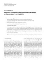
interpolated SCM. Figure 2 plots the absolute values of the
resulting spatial CCFs at the BS (AS
= 2
◦
for macrocell and
AS
= 5
◦
for microcell) and MS (AS = 35
◦
) as functions of the
normalized antenna spacings Δd
s
/λ and Δd
u
/λ,respectively,
for both the SCM and interpolated SCM. In this figure, we
also include the corresponding absolute values of the spatial
CCFs for the KBSM with uniform, truncated Gaussian, and
truncated Laplacian subpath PASs. Note that the method of
6 EURASIP Journal on Wireless Communications and Networking
151050
Normalized antenna spacing, Δd
u

/λ or Δd
s
/λ
0
0.2
0.4
0.6
0.8
1
1.2
Absolute value of the cluster-level spatial CCF
KBSM with uniform subpath PASs
KBSM with Gaussian subpath PASs
KBSM with Laplacian subpath PASs
SCM
Interpolated SCM
AS
= 2
AS = 5
AS = 35
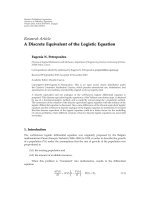
Figure 2: The absolute values of the cluster-level spatial CCFs of the
SCM, interpolated SCM, and KBSMs with uniform, Gaussian, and
Laplacian subpath PASs (mean AoA/AoD
= 60
◦
).
Bessel series expansion [20] was applied here to calculate (13)
and (14) for the KBSM. From Figure 2, the following obser-
vations can be obtained: (1) the KBSM with the truncated
Gaussian subpath PASs provides the best fitting to both the

SCM and interpolated SCM. This is interesting by consid-
ering the fact that the 3GPP actually suggested a Laplacian
distribution for the AoD PAS and either a Laplacian or a uni-
form distribution for the AoA PAS in its link-level calibra-
tion [14]. However, this observation conforms to the mea-
surement result in [26], where a Gaussian PDF was found
to best match the measured azimuth PDF. (2) A larger AS
results in smaller spatial correlations. The same conclusion
was also mentioned in [7]. (3) The spatial CCFs at the BS,
that is, AS
= 2
◦
and 5
◦
, of the SCM can match well the cor-
responding ideal values, approximated here by those of the
interpolated SCM. However, the spatial CCF at the MS, that
is, AS
= 35
◦
, of the SCM fluctuates unstably around that of
the interpolated SCM. This is caused by the so-called “im-
plementation loss” due to the insufficient number M of sub-
paths used in the SCM. It is therefore suggested that in the
3GPP SCM, the employed number of subpaths M
= 20 is
not sufficient and should be increased in order to improve
its simulation accuracy of the cluster level spatial CCF at
the MS. In the following, using the same parameter gener-
ating procedure [14, 27], we will compare the spatial CCFs

ρ
s
1
u
1
s
2
u
2
(Δd
s
, Δd
u
)in(6), ρ
MS
u
1
u
2
(Δd
u
)in(7), and ρ
BS
s
1
s
2
(Δd
s
)in(8)

of the SCM with
ρ
s
1
u
1
s
2
u
2
(Δd
s
, Δd
u
)in(15), ρ
MS
u
1
u
2
(Δd
u
)in(13),
and
ρ
BS
s
1
s
2

(Δd
s
)in(14) of the KBSM having Gaussian subpath
PASs at the three levels. The normalized BS antenna spacing
Δd
s
/λ = 1 was chosen to calculate (6), (8), (14), and (15),
10.80.60.40.20
Absolute value of the cluster-level spatial CCF of the KBSM
0
0.1
0.2
0.3
0.4
0.5
0.6
0.7
0.8
0.9
1
Absolute value of the cluster-level spatial CCF of the SCM
ρ
BS
s
1
s
2
and ρ
BS
s

1
s
2
ρ
MS
u
1
u
2
and ρ
MS
u
1
u
2
ρ
s
1
u
1
s
2
u
2
and ρ
s
1
u
1
s

2
u
2
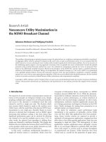
Figure 3: The absolute values of the cluster-level spatial CCFs of the
SCM and KBSM with Gaussian subpath PASs (Δd
s
/λ = 1, Δd
u
/λ =
1, BS AS = 5
◦
,MSAS= 35
◦
).
while the normalized MS antenna spacing Δd
u
/λ = 1 was se-
lected for computing (6), (7), (13), and (15). The subpath an-
gle offsets Δ
n,m,AoD
and Δ
n,m,AoA
of the SCM were taken from
Table 1 with AS
= 5
◦
and AS = 35
◦
,respectively.
Figure 3 compares the absolute values of the cluster-

level spatial CCFs of the SCM and KBSM. Forty constant
values were taken from [0, 90
◦
) for both the mean AoD
(θ
n,AoD
,

θ
0,AoD
)andmeanAoA(θ
n,AoA
,

θ
0,AoA
). From this
figure, it is obvious that ρ
BS
s
1
s
2
(Δd
s
) ≈ ρ
BS
s
1
s

2
(Δd
s
) holds since
all the values are located in the diagonal line. The relatively
small difference between ρ
MS
u
1
u
2
(Δd
u
)andρ
MS
u
1
u
2
(Δd
u
)comes
mostly from the above-mentioned “implementation loss.”
On the other hand, ρ
s
1
u
1
s
2

u
2
(Δd
s
, Δd
u
)differs significantly from
ρ
s
1
u
1
s
2
u
2
(Δd
s
, Δd
u
). This clearly tells us that the fundamental dif-
ference exists between the SCM and KBSM at the cluster
level since the spatial separability is not fulfilled for the SCM.
Figure 4 illust rates the absolute values of the link level spa-
tial CCFs versus the normalized MS antenna spacing Δd
u
/λ
for both the SCM and KBSM. Here, θ
BS
= 50

◦
, θ
MS
=
195
◦
, δ
n,AoD
=

δ
AoD
are considered as uniformly distributed
random variables located in the interval [
−40
◦
,40
◦
), while
δ
n,AoA
=

δ
AoA
are Gaussian distributed random variables
[14]. To calculate the average in (6)and(7), 1000 random re-
alizations of the cluster position parameters δ
n,AoD
and δ

n,AoA
were used. Clearly, good agreements are found in terms of
the link-level spatial CCFs between the SCM and KBSM. It
follows that the SCM has the same property of the spatial
separability as the KBSM at the link-level. In Figure 5,we
demonstrate the absolute values of the system level spatial
CCFs versus the normalized MS antenna spacing Δd
u
/λ for
Cheng-Xiang Wang et al. 7
1.510.50
Normalized MS antenna spacing, Δd
u
/λ
0
0.2
0.4
0.6
0.8
1
Abosolute value of the link-level spatial CCF
ρ
MS
u
1
u
2
and ρ
MS
u

1
u
2
ρ
s
1
u
1
s
2
u
2
and ρ
s
1
u
1
s
2
u
2
SCM
KBSM
Figure 4: The absolute values of the link-level spatial CCFs of the
SCM and KBSM with Gaussian subpath PASs (Δd
s
/λ = 1, θ
BS
= 50
◦

,
θ
MS
= 195
◦
,BSAS= 5
◦
,MSAS= 35
◦
).
1.510.50
Normalized MS antenna spacing, Δd
u
/λ
0
0.2
0.4
0.6
0.8
1
Abosolute value of the system-level spatial CCF
ρ
MS
u
1
u
2
and ρ
MS
u

1
u
2
ρ
s
1
u
1
s
2
u
2
and ρ
s
1
u
1
s
2
u
2
SCM
KBSM
Figure 5: The absolute values of the system-level spatial CCFs of
the SCM and KBSM with Gaussian subpath PASs (Δd
s
/λ = 1, BS
AS
= 5
◦

,MSAS= 35
◦
).
both the SCM and KBSM. The cluster position parameters
δ
n,AoD
=

δ
AoD
and δ
n,AoA
=

δ
AoA
are still random variables
following the corresponding distributions in the link level,
while both θ
BS
=

θ
BS
and θ
MS
=

θ
MS

areconsideredasran-
dom variables uniformly distributed over [0, 2π)[14]. Again,
the system-level spatial CCFs of the SCM match very closely
those of the KBSM. The conclusion we can draw is that the
spatial separability is also a property of the SCM at the system
level.
43210
Normalized time delay,
v τ/λ
0
0.2
0.4
0.6
0.8
1
Absolute value of the temporal ACF
KBSM
System-level SCM
Link-level SCM
Cluster-level SCM
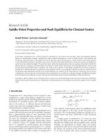
Figure 6: The absolute v alues of the temporal ACFs of the KBSM
and SCM at the cluster level, link level, and system level (θ
v
= 60
◦
).
To summarize, the KBSM has the property of the spatial
separability at all the three levels, while the SCM exhibits the
spatial separability only at the link and system levels, not at
the cluster level.

4.2. Temporal ACFs
ThetemporalACF
r(τ) = J
0
(2πvτ/λ) of the KBSM re-
mains static at all the three levels. For the SCM, however,
the expression (12) clearly shows that r(τ)variesatdiffer ent
levels. Figure 6 compares the absolute values of the temporal
ACFs of the KBSM and SCM at the three levels. For the cal-
culation of (12), θ
v
= 60
◦
and the rest angle parameters at
different levels were taken as specified in Section 4.1.Asex-
pected, the temporal ACFs of the SCM at the cluster level or
link level show substantial variations across different runs. At
the system level, both models tend to have the identical ACFs.
This indicates that the spatial-temporal separability is ful-
filled for the SCM only a t the system level, not at the cluster
and link levels. In the case of the KBSM, the spatial-temporal
separability is always its property at any level. Hence, the
KBSM actually only models the average spatial-temporal be-
havior of MIMO channels, while the SCM provides us with
more detailed information about variations across different
realizations of MIMO channels. Clearly, a single KBSM is not
sufficient for system-level simulations.
5. CONCLUSIONS
In this paper, we have proposed to compare the spatial-
temporal correlation chara cteristics of the 3GPP SCM and

KBSM at three levels. Theoretical studies clearly show that
the spatial CCF of the SCM is related to the joint distribu-
tion of the AoA and AoD, while the KBSM calculates the
8 EURASIP Journal on Wireless Communications and Networking
spatial CCF from independent AoA and AoD distributions.
Under the conditions that the number of subpaths tends to
infinity in the SCM, two correlated links share one antenna
at either end, and the same set of angle parameters is used,
the two models tend to be equivalent. Compared with uni-
form and Laplacian functions, it turns out that the Gaussian-
shaped subpath PAS enables the KBSM to best fit the 3GPP
SCM in terms of the spatial CCFs. It has also been demon-
strated that the spatial separability is observed for the SCM
only at the link and system levels, not at the cluster level.
The spatial-temporal separability is a property of the SCM
only at the system level, not at the cluster and link levels. The
KBSM, however, exhibits both the spatial separability and the
spatial-temporal separability at all the three levels.
Although the KBSM has the advantages of simplicity and
analytical tr actability, it only describes the average spatial-
temporal properties of MIMO channels. On the other hand,
the SCM is more complex but allows us to sufficiently sim-
ulate the variations of different MIMO channel realizations.
Therefore, the SCM gives more insights of MIMO channel
mechanisms. A tradeoff between model accuracy and com-
plexity must be considered in terms of the use of the SCM
and KBSM.
ACKNOWLEDGMENT
The authors appreciate the helpful comments from Dr. Dave
Laurenson, University of Edinburgh, UK.

REFERENCES
[1] I. E. Talatar, “Capacity of multi-antenna Gaussian channels,”
Tech. Rep., AT&T Bell Labs, Florham Park, NJ, USA, June
1995.
[2] G. J. Foschini and M. J. Gans, “On limits of wireless commu-
nications in a fading environment when using multiple an-
tennas,” Wireless Personal Communications,vol.6,no.3,pp.
311–335, 1998.
[3] V. Tarokh, H. Jafarkhani, and A. R. Calderbank, “Space-time
block codes from orthogonal designs,” IEEE Transactions on
Information Theory, vol. 45, no. 5, pp. 1456–1467, 1999.
[4] G. J. Foschini, “Layered space-time architecture for wireless
communication in a fading environment when using multi-
element antennas,” Bell Labs Technical Journal,vol.1,no.2,
pp. 41–59, 1996.
[5] H. B
¨
olcskei and A. J. Paulraj, “Space-frequency coded broad-
band OFDM systems,” in Proceedings of the IEEE Wireless Com-
munications and Networking Conference (WCNC ’00), vol. 1,
pp. 1–6, Chicago, Ill, USA, September 2000.
[6] D S. Shiu, G. J. Foschini, M. J. Gans, and J. M. Kahn, “Fading
correlation and its effect on the capacity of multielement an-
tenna systems,” IEEE Transactions on Communications, vol. 48,
no. 3, pp. 502–513, 2000.
[7] J.P.Kermoal,L.Schumacher,K.I.Pedersen,P.E.Mogensen,
and F. Frederiksen, “A stochastic MIMO radio channel model
with experimental validation,” IEEE Journal on Selected Areas
in Communications, vol. 20, no. 6, pp. 1211–1226, 2002.
[8] A. Abdi, J. A. Barger, and M. Kaveh, “A parametric model for

the distribution of the angle of arrival and the associated cor-
relation function and power spectrum at the mobile station,”
IEEE Transactions on Vehicular Technology,vol.51,no.3,pp.
425–434, 2002.
[9] L. Schumacher, L. T. Berger, and J. Ramiro-Moreno, “Recent
advances in propagation characterisation and multiple an-
tenna processing in the 3GPP framework,” in Proceedings of
the 26th General Assembly of International Union of Radio Sci-
ence (URSI ’02), Maastricht, The Netherlands, August 2002.
[10] A. Abdi and M. Kaveh, “A space-time correlation model for
multielement antenna systems in mobile fading channels,”
IEEE Journal on Selected Areas in Communications, vol. 20,
no. 3, pp. 550–560, 2002.
[11] G. J. Byers and F. Takawira, “Spatially and temporally corre-
lated MIMO channels: modeling and capacity analysis,” IEEE
Transactions on Vehicular Technology, vol. 53, no. 3, pp. 634–
643, 2004.
[12] M. Lu, T. Lo, and J. Litva, “A physical spatio-temporal model
of multipath propagation channels,” in Proceedings of the 47th
IEEE Vehicular Technology Conference (VTC ’97), vol. 2, pp.
810–814, Phoenix, Ariz, USA, May 1997.
[13] 3GPP, R1-02-0181, “MIMO discussion summary,” January
2002.
[14] 3GPP, TR 25.996, “Spatial channel model for multiple input
multiple output (MIMO) simulations (Rel. 6),” 2003.
[15] 3GPP, R1-050586, “Wideband SCM,” 2005.
[16] L. Correia, Wireless Flexible Personalised Communications—
COST 259 Final Report, John Wiley & Sons, New York, NY,
USA, 2001.
[17] P. J. Smith and M. Shafi, “The impact of complexity in MIMO

channel models,” in Proceedings of IEEE International Con-
ference on Communications (ICC ’04), vol. 5, pp. 2924–2928,
Paris, France, June 2004.
[18] A. Giorgetti, P. J. Smith, M. Shafi, and M. Chiani, “MIMO
capacity, level crossing rates and fades: the impact of spa-
tial/temporal channel correlation,” Journal of Communications
and Networks, vol. 5, no. 2, pp. 104–115, 2003.
[19] H. Xu, D. Chizhik, H. Huang, and R. Valenzuela, “A gen-
eralized space-time multiple-input multiple-output (MIMO)
channel model,” IEEE Transactions on Wireless Communica-
tions, vol. 3, no. 3, pp. 966–975, 2004.
[20] L. Schumacher, K. I. Pedersen, and P. E. Mogensen, “From an-
tenna spacings to theoretical capacities - guidelines for simu-
lating MIMO systems,” in Proceedings of the 13th Annual IEEE
International Symposium on Personal Indoor and Mobile Ra-
dio Communications (PIMRC ’02)
, vol. 2, pp. 587–592, Lisbon,
Portugal, September 2002.
[21] W. C. Y. Lee, “Effects on correlation between two mobile radio
base-station antennas,” IEEE Transactions on Communications,
vol. 21, no. 11, pp. 1214–1224, 1973.
[22] F. Adachi, M. Feeny, A. Williamson, and J. Parsons, “Crosscor-
relation between the envelopes of 900 MHZ signals received
at a mobile radio base station site,” IEE Proceedings—Part F:
Communications, Radar and Signal Processing, vol. 133, no. 6,
pp. 506–512, 1986.
[23] J. Salz and J. H. Winters, “Effect of fading correlation on adap-
tive arrays in digital mobile radio,” IEEE Transactions on Vehic-
ular Technology, vol. 43, no. 4, pp. 1049–1057, 1994.
[24] K. I. Pedersen, P. E. Mogensen, and B. H. Fleury, “Spatial chan-

nel characteristics in outdoor environments and their impact
on BS antenna system performance,” in Proceedings of the 48th
IEEE Vehicular Technology Conference (VTC ’98), vol. 2, pp.
719–723, Ottawa, Canada, May 1998.
Cheng-Xiang Wang et al. 9
[25] W. C. Jakes, Ed., MicrowaveMobileCommunications, IEEE
Press, Piscataway, NJ, USA, 1994.
[26] K.I.Pedersen,P.E.Mogensen,andB.H.Fleury,“Astochas-
tic model of the temporal and azimuthal dispersion seen at
the base station in outdoor propagation environments,” IEEE
Transactions on Vehicular Technology, vol. 49, no. 2, pp. 437–
447, 2000.
[27] J. Salo, G. Del Galdo, J. Salmi, et al., “MATLAB implementa-
tion of the 3GPP Spatial Channel Model (3GPP TR 25.996),”
January 2005, .fi/Units/Radio/scm.