Báo cáo hóa học: " Research Article Communication Timing Control with Interference Detection for Wireless Sensor Networks" potx

Hindawi Publishing Corporation
EURASIP Journal on Wireless Communications and Networking
Volume 2007, Article ID 54968, 10 pages
doi:10.1155/2007/54968
Research Article
Communication Timing Control with Interference
Detection for Wireless Sensor Networks
Yuki Kubo
1, 2
and Kokuke Sekiyama
3
1
Ubiquitous System Laboratory, Corporate Research and Development Center, OKI Electric Industry Co., Ltd.,
2-5-7 Honmachi, Chuo-Ku, Osaka-Shi, Osaka 541-0053, Japan
2
Department of System D e sign Engineering, University of Fukui, 3-9-1 Bunkyo, Fukui-Shi, Fukui 910-8507, Japan
3
Department of Micro-Nano Systems Engineering, Nagoya University, Furo-Cho, Chikusa-Ku, Nagoya 464-8603, Japan
Received 31 May 2006; Revised 16 October 2006; Accepted 18 October 2006
Recommended by Xiuzhen Cheng
This paper deals with a novel communication timing control for wireless networks and radio interference problem. Communica-
tion timing control is based on the mutual synchronization of coupled phase oscillatory dynamics with a stochastic adaptation,
according to the history of collision frequency in communication nodes. Through local and fully distributed interactions in the
communication network, the coupled phase dynamics self-organizes collision-free communication. In wireless communication,
the influence of the interference wave causes unexpected collisions. Therefore, we propose a more effective timing control by se-
lecting the interaction nodes according to the received signal strength.
Copyright © 2007 Y. Kubo and K. Sekiyama. This is an open access article distributed under the Creative Commons Attribution
License, which permits unrestricted use, distribution, and reproduction in any medium, provided the original work is properly
cited.
1. INTRODUCTION
In recent years, research on wireless sensor networks has been

promoted rapidly [1]. The sensor networks are composed of
distributed sensor devices connected with wireless commu-
nication and sensing functions. Potential application fields
of the sensor networks include stock-management systems,
road traffic surveillance systems, and air-conditioning con-
trol systems of a large-scale institution and so on. There are
many technical issues in the sensor networks. In this paper,
we deal with two problems. One of them is a communica-
tion timing control for collision avoidance. Another is the
influence of interference wave on the communication timing
control. In order to cope with malfunctions and changes of
the number of active sensor nodes, a distributed autonomous
communication timing control is preferable to centralized
approaches which must rely on a fixed base station in general.
In order to avoid the collision issue, TDMA [2]system
has been presented, which is a multiplexing technology in
the time domain that makes it possible to avoid collisions by
assigning a communication slot to one frame. Hence, no col-
lision occurs, and any node can obtain impartial communi-
cation rig ht in TDMA. TDMA is widely used in cellular tele-
phone systems. However, TDMA is fundamentally a central-
ized management technique depending on a base station and
is applicable to a star link network. Meanwhile, distributed
slot assignment TDMA approach for ad hoc networks has
been proposed. In Ephremides and Truong algorithm [3],
allocation of one transmission slot is assured for each node
by preparing N slots for N nodes. In addition, it is possible
to add more slot allocations by referring to information of
the slot allocation within the two hop nodes for the collision
avoidance based on the distributed algorithm. However, this

algorithm requires total number of the node. Hence, this al-
gorithm has a limitation in changing the number of nodes
flexibly. USAP-MA [4] deals with a distributed slot assign-
ment in TDMA for changes of the number of nodes. This
method provides a dynamic change of frame length corre-
sponding to the number of nodes and network topology, and
improves bandwidth efficiency. Also, the other methods of
slot reservation have been proposed for TDMA [ 4–6]. How-
ever, these TDMA-based approaches require a global time
synchronization.
As another collision avoidance technique, CSMA [7, 8]
has been widely used. CSMA is a simple and scalable pro-
tocol. In the case of low-traffic situation, CSMA works effi-
ciently. However, according to the increase of nodes, commu-
nication throughput sharply declines due to occurrence of
2 EURASIP Journal on Wireless Communications and Networking
9
4
0
2
11
5
1
6
10
8
3
7
12
(a)

φ
c
Δθ
ij
11 4
2
3
9
8
6
10
1
5
12
0
7
Initial state Convergence state
12
5
2
φ
c
0
9
6
3
10
7
4
1

8
11
(b)
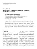
Figure 1: (a) Node arrangement and communication range; (b) phase pattern formation for collision avoidance.
frequent packet collisions. Such collisions should be avoided
for not only improvement of the throughput efficiency, but
also saving the electric energy consumption required in the
retransmissions. Furthermore, several problems are pointed
out with regard to the cost of carrier sense [9] and hidden ter-
minals [7, 8]. Also, with the CSMA-based approach, it is diffi-
cult to ensure impartial communication right because of the
high contention of nodes that share communication channel.
Other research in the wireless sensor networks includes
SMAC [10], SMACS [11]. SMAC is based on CSMA, where
each node broadcasts a sleep timing schedule to the neigh-
bor nodes. The nodes receiving this message are to adjust
the schedule of sleep, by which a node can save energy con-
sumption. Although the problem of collision is inevitable,
the aim of this research is focused on a timing control for en-
ergy saving. Hence, fundamental problems in CSMA remain
unsolved. SMACS realizes an efficient communication based
on synchronization between two nodes. These nodes attempt
to schedule a communication timing with each other. Ad-
ditionally, each node utilizes a different frequency band for
adifferent link for collision avoidance. In this method, the
risk of collisions can be reduced by random sharing of the
frequency band. SMACS is different from the basic TDMA
in that synchronization is required between two correspond-
ing nodes while TDMA requires global synchronization. In
general, global synchronization without a base station is hard

to achieve. We have proposed a distributed communication
timing control for collision avoidance named phase diffu-
sion time-division method (PDTD) [12]. This method is a
distributed communication timing control based on the dy-
namics of coupled phase oscillator among the peripheral
nodes. Through local and fully distributed interactions, the
coupled phase dynamics self-organizes the effective phase
synchronous state that allows collision-free communication.
On the other hand, radio interference is an important
problem in the wireless communication. Interference prob-
lems include two kinds of problems. One of them is to re-
duce influence of interference. Another problem concerns
the communication timing under the influence of interfer-
ence. Radio interference greatly influences the communica-
tion protocol [13]. Decentralized scheduling TDMA is based
on the graph structure of the node connection within com-
munication range. The issue of radio interference is not con-
sidered in decentralized scheduling TDMA. Therefore, in the
presence of interference wave, it may not be an appropri-
ate schedule method when considering the issue of inter-
ference. Also, in the case of CSMA-based protocol, hidden
terminal collision avoidance mechanism based on RTS and
CTS messages will not work appropriately [14]. In the previ-
ous timing control based on PDTD, we did not deal with ra-
dio interference problems. Therefore, unexpected collisions
may occur in the real environment. In this paper, we pro-
pose the extended version of PDTD with interference de-
tection (PDTD/ID). Each node exchanges the received sig-
nal strength and specifies the interference source node. This
has to be incorporated for interaction nodes for collision

avoidance in PDTD. We verify the efficiency of the proposed
method by simulation experiments.
2. COMMUNICATION TIMING CONTROL
2.1. Outline of PDTD
In this section, we will review a basic concept of PDTD. We
assume a situation in which a node periodically transmits
data. The node is modeled as an oscillator that periodically
repeats the states of the communication and noncommu-
nication. Hence, mutual adjustment of the communication
timing is formulated based on the coupled oscillator dynam-
ics. The communication timing state of the node is expressed
as a phase. The phase of the oscillator for node i is denoted
as θ
i
, and angular velocity is ω
i
. We suppose that each node
can transmit data only within the phase interval 0 <θ
i
<φ
c
as depicted in Figure 1. If other nodes do not transmit in the
interval 0 <θ
i
<φ
c
, no collision occurs. Figure 1 shows the
phase relation from the viewpoint of node 0. Figure 1(left)
depicts initial state. In this case, the phase difference is not
large enough, hence a collision occurs. If each node forms ap-

propriate communication timing like Figure 1(right), colli-
sion does not occur. The node transmits the control message
Y. Kubo and K. Sekiyama 3
4
5
2
Control
message
3
1
6
7
(a) Node arrangement and communica-
tion range
3
7
5
Node 2
φ
c
1
6
2
θ
2
4
3
7
5
Node 1

φ
c
1
6
2
θ
1
4
Self
1hop
2hops
(b) Sending phase value by control message
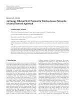
Figure 2: Node interaction based on control message.
at θ
i
= 0 for communication timing control. Each node is as-
sumed to know the phase value of the neighbor nodes by re-
ceiving the control message, and to calculate phase dynamics.
2.2. Node interaction
We explain the method of exchanging phase value with each
other by the control message. The control message from node
i includes the following information:
(1) one-hop neighbor node ID j
= (0,1,2, );
(2) phase value of one-hop neighbor (

θ
i0
,


θ
i1
,

θ
i2
, ,

θ
ij
);
(3) received signal strength value from one-hop neighbor
(P
i 0
, P
i 1
, P
i 2
, , P
i j
).
The phase value of one-hop neighbor is used for calcula-
tion of communication timing control. The received signal
strength value is used for selection of interference nodes.
These are detailed in Sections 2.3 and 3. Since the control
messages are transmitted by the same channel with the data
messages, there is possibility that the control messages might
be occasionally lost by collisions. However, the transmission
of the control messages is executed periodically, it is unlikely
that the control message is lost every time.

The process to convey node information to the neigh-
boring nodes is explained as follows. The node is assumed
to be able to know only its self phase value when calculat-
ing phase dynamics. However, the node estimates the phase
value of the neighboring nodes from their control mes-
sages. In this paper, the neighbor node of which informa-
tion is temporarily generated based on this estimation is
called a virtual node. The node controls communication tim-
ing by the interaction with a virtual node. Figures 2(a) and
2(b) show the case that node 2 transmits the control mes-
sage. Figure 2(a) shows node allocation and communication
range. Figure 2(b) shows the state of virtual nodes of nodes 1
and 2 corresponding to Figure 2(a). The interaction process
of nodes 1 and 2 is as follows. Node 2 transmits the control
message at phase θ
2
= 0, then the control message includes
information of nodes 1, 3, 4, and 5 that exist in one-hop
neighbor. Node 1 that received this massage generates virtual
nodes corresponding to nodes 1, 2, 3, 4, and 5 listed i n con-
trol message from node 2. The phase with dashed circle in
Figure 2(b) denotes the corresponding node. A virtual node
corresponding to node 2 (sender of the control message) is
registered as one-hop neighbor node. Nodes 3, 4, and 5 (the
other nodes contained in the control message) are registered
as two-hop neighbor nodes. In this regard, node 3 is classi-
fied as the two-hop neighbor node from node 1. However, if
node 1 is able to communication directly with node 3, node
3 is registered as the one-hop neighbor node. Through send-
ing and receiving of a periodic control message, each node

has node information within two-hop neighbor nodes as a
virtual node.
2.3. Communication timing control based on PDTD
Coupled phase dynamics
PDTD provides communication timing control based on
phase dynamics for collision avoidance. Node i interacts with
a virtual node and forms appropriate phase-difference pat-
tern. Let

θ
ij
denote phase value of virtual node j for node i.
Then the governing equation is given by the following equa-
tions:
dθ
i
dt
= ω
i
+

j K
i
k
j
R

Δ

θ

ij

+ ξ

S
i

,(1)
Δ

θ
ij
=

θ
ij
θ
i
,(2)
d

θ
ij
dt
= ω
ij
,(3)
where ω
i
and ω

ij
denote the angular velocity of node i and
virtual node j,respectively,andk
j
is the coupled strength
value. K
i
is a virtual node set of node i. Every node is allowed
to transmit data for φ
c
/ω
i
(s) every cycle. ξ(S
i
) is a stochastic
term, details of w hich are explained in Section 2.3.Interac-
tion with the neighbor nodes is governed by phase-response
4 EURASIP Journal on Wireless Communications and Networking
function R(Δ

θ
ij
) which is a repulsive function as follows:
R

Δθ
ij

=
⎧

⎪
⎪
⎨
⎪
⎪
⎩
Δθ
ij
φ
c
, Δθ
ij
φ
c
,
0, φ
c
< Δθ
ij
< 2π φ
c
,
Δθ
ij
2π + φ
c
,2π φ
c
Δθ
ij

.
(4)
Stochastic adaptation
When relying only on the repulsive interaction, the phase-
difference pattern often fails to converge to the desired sta-
tionary state. Therefore, a stochastic adaptation term ξ(S
i
)is
introduced, which is determined by the estimated risk of the
collision. As an evaluation index, phase overlap rate is de-
fined. Node communication state is defined such that O
i
= 1
denotes that node i is allowed to communicate, and O
i
= 0
denotes that node i is prohibited to communicate, which is
given by
O
i

θ
i
(t)

=
⎧
⎨
⎩
1, 0 θ

i
<φ
c
,
0, φ
c
θ
i
< 2π.
(5)
Flag function to indicate phase overlap of communication
timing between node i and virtual nodes is given by
x
i
(t) =
⎧
⎪
⎨
⎪
⎩
1, O
i

θ
i

=
1,

j K

i
O
j


θ
ij

> 0,
0 else.
(6)
x
i
= 1 indicates that there is a phase overlap that would cause
a collision. If

t+T
t
x
i
(t) = 0, then one collision is counted for
one cycle. Let γ indicate the occurrence time of phase overlap
for past n cycles. overlap rate c
i
is given by
c
i
(t) =
γ
n

. (7)
The stress of being exposed to the risk of collision is accumu-
lated by the following mechanism:
S
i
(t) = 2S
i
(t τ)+s

c
i

,
s

c
i

=
⎧
⎪
⎪
⎪
⎪
⎪
⎪
⎪
⎪
⎨
⎪

⎪
⎪
⎪
⎪
⎪
⎪
⎪
⎩
0.0, 0 c
i
< 0.2,
0.03, 0.2
c
i
< 0.5,
0.05, 0.5
c
i
< 0.8,
0.1, 0.8
c
i
< 0.9,
0.3, 0.9
c
i
,
(8)
where τ
= n T

i
is a stress accumulating time scale. Random
phase jump is implemented every n
T
i
[s] cycles with prob-
ability S
i
,whereifS
i
> 1, then S
i
1. After random phase
jump, then S
i
0. The destination of phase jump is decided
as follows. Assume that node i has

N
i
virtual nodes, the phase
of which is denoted as

θ
ij
. Sorting the phase value

θ
ij
in as-

cending order, such as

θ
(1)
il
< <

θ
(k)
ij
< <

θ
(

N
i
)
ik
, the
corresponding node to kth phase value is v
k
. T he destination
of stochastic jump is depicted as shown in Figure 3. The list
of destination u
k
is given by
u
k
=

v
k
+ v
k+1
2

k = 1, 2, ,

N
i
1

. (9)
0
v
1
v
2
v
3
v
4
v
5
v
6
2π
u
1
u

2
u
3
u
4
u
5
Figure 3: Destination list of random phase jump.
The preferential selection probability u
k
is decided by the
equation
p
k
=
exp

β

v
k+1
v
k



N
i
1
l

=1
exp

β

v
l+1
v
l


l = 1, 2, ,

N
i
1

,
(10)
where β is a sensitivity par ameter of the selection.
3. COMMUNICATION TIMING CONTROL WITH
INTERFERENCE NODE DETECTION
3.1. Radio interference problem
In a wireless communication, even in the presence of weak
interference wave, a node may fail to communicate if the
desired wave strength from the node is weak. On the other
hand, if the desired wave strength is sufficiently strong, the
node may be able to receive data from the other node suc-
cessfully despite presence of a strong interference wave. The
reception error caused by an interference wave is estimated

by signal-to-interference ratio (SIR). The threshold of SIR to
correctly receive a signal is determined by modulation meth-
ods and spec of the receiver. In the communication timing
control described in Section 2.3 , however, the influence of in-
terference wave was not taken into account in our model. In
spite of the assumption that the interaction range is within
the two-hop neighbors, interference waves can be reached
beyond the interaction range, and hence this could cause un-
expected collisions. Therefore, each node has to select the in-
teraction nodes based on the relation between received signal
wave strength and interference wave strength.
3.2. Radio interference model
In this section, we discuss how the interference source is
specified based on the received electric power. As shown in
Figure 4,nodesi, j,andk are placed, where the internode
distance between nodes i and j and the one between nodes j
and k are denoted by d
s
, d
i
, respectively. The interference oc-
curs in node j when node i transmits to node j. Also assume
that all nodes transmit in the same electric power t
p
(mW).
The received electric power p(d)(mW) is assumed available
by the following equation [14]:
p(d)
=
c t

p
d
α
, (11)
where d is the distance between the sender node and the re-
ceiver node. α is the signal attenuation coefficient. c is the
combined parameter that is related to the reception strength.
Assume that node i is the transmitting source, and node k is
Y. Kubo and K. Sekiyama 5
k
ij
p(d
s
)
d
s
p(d
i
)
d
i
Figure 4: The existence range of interference source (ERIS).
an interference source. With (11), SIR is defined as the ratio
of the electric power between the desired signal from node i
and the interference wave from node k;
SIR
=
p

d

s

p

d
i

=

d
i
d
s

α
. (12)
SIR has to be bigger than the threshold e
sir
in order for the
transmission from node i to be successfully received in node
j. Otherwise, in the case of SIR
e
sir
, the interference would
occur in node j, and node k is referred to as the interference
source node for node j. In general, the existence range of in-
terference source node is given by the foll owing equation:
d
i
α

e
sir
d
s
. (13)
We call the existence range of interference source node as
ERIS in the follow ing section. It can be said that ERIS is pro-
portional to the distance d
s
by (13). In order for node i to be
able to communicate with node j successfully, node i has to
specify which node can be the interference node for node j.
Such nodes are referred to as the interference source nodes.
Node i is not allowed to transmit at the same time as the in-
terference source node.
3.3. Interference node detection
Existence range of interference source
As mentioned in the previous section,
SIR
=
p

d
s

p

d
i


>e
sir
(14)
is required for successful communication in the presence of
interference waves. Taking logarithm in (14), we obtain
P
s
P
i
>E
sir
, (15)
where P
s
= 10 log
10
p(d
s
), P
i
= 10 log
10
p(d
i
), and E
sir
=
10 log
10
e

sir
. Figure 5 shows the existence range of interfer-
ence source (ERIS). Let P
min
(dBm) be the minimum received
signal strength for a successful communication. In the case
P
i
= P
min
E
sir
P
i
= P
min
31
2
P
c
P
min
Figure 5: Limitation of destination node and ERIS.
that node 1 transmits to node 2 that is located on the bound-
ary of communication range from node 1, the received signal
strength on the boundary positions will become P
min
(dBm).
Hence, it is supposed that P
s

= P
min
in (15), then P
min
E
sir
>
P
i
is derived, which indicates that node 2 will fail to receive
the transmission from node 1, if the strength of interference
wave is larger than P
i
= P
min
E
sir
(dBm). The ERIS, the
corresponding range for P
i
, will become larger than the com-
munication range of node 2. Therefore, some extension is re-
quired for the timing control with two-hop neighbor nodes
based on the PDTD because the interference wave may cause
another collision. On the other hand, when node 1 transmits
to node 3, which is closer than node 2, assume that node 3 re-
ceives the signal of st rength P
c
= P
min

+E
sir
(dBm). This is the
case of P
s
= P
c
in (15), where since P
c
E
sir
>P
i
, P
min
>P
i
is obtained. This implies that the ERIS (P
i
) is the same or
inside of the communication range of node 3. Therefore, if
the communication range is redefined as P
c
instead of P
min
,
it is possible to avoid the problem caused by the interference
wave in PDTD.
Detection process of interference node
In this section, the process of interference node detection is

addressed. This method is based on the evaluation of the re-
ceived signal strength, where two different scenarios can be
considered. The first case is that when node a transmits to
node b, the interference occurs in the destination node b be-
cause of transmissions from some other nodes. In this case,
node a needs to specify which nodes are causing the inter-
ference to node b (detection of the interference nodes), in
an attempt to execute the timing control with such interfer-
ence nodes. On the other hand, the second case is that the
transmission from node a to a destination node c is causing
an interference to node b,wherenodea is becoming an in-
terference node for node b unintentionally, and such a node
could exist many around node a.Hence,nodea is asked to
specify the node set that can be interfered by the transmission
of node a, and conduct a timing control with those nodes to
avoid a potential collision.
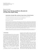
ThefirstcaseisexemplifiedinmoredetailinFigure 6(a),
where node 1 receives a control message from node 2 with
the signal strength larger than P
c
(dBm) in an attempt to
6 EURASIP Journal on Wireless Communications and Networking
17
10
6
16
2
7
3
8

1
5
E
sir
13 14
9
12
11
15
4
P
2 1
P
c
P
min
(a) A case that node 1 receives control mes-
sage from node 2 with signal strength larger than
P
c
(dBm)
17
10
6
16
2
7
3
8
1

5
+E
sir
13
14
9
12
11
15
4
P
9 1
P
c
P
min
(b) A case that node 1 receives control mes-
sage from node 9 with signal strength less than
P
c
(dBm)
Figure 6: Interference node selection based on received signal strength.
specify the interference nodes for node 2. As described in
Section 2.2, the control message from node 2 includes the
signal strength data which had been received by node 2 from
the other nodes. In Figure 6(a), this control message includes
datafromnodes1,3,4,5,6,7,8,and10.
Let P
b a
denote the received signal strength of node b

from node a, then node 1 compares P
2 1
(the desired sig-
nal) with P
2 x
,(x = 3, 4, 5, 6, 8, 10) in order to judge as to
whether each node x would become the interference source.
From (15), if P
2 1
P
2 x
E
sir
,nodex may cause the inter-
ference to node 2. Such a node set is defined as
L
I
(b a) =

x P
b x
P
b a
E
sir
, x = a

.
(16)
Equation (16) represents the node set that could cause the

interference to node b when node a transmits to node b.It
should be noted that the node set L
I
(b a) is determined
by node a based on the control message from node b,hence
node a is excluded from the set L
I
(b a). As depicted in
Figure 6(a), L
I
(2 1) = 3,4, 5, 6, 7 that are the nodes in-
side the range of dashed circle, P
2 1
E
sir
. While, the sec-
ond scenario is exemplified in Figure 6(b) where there is no
direct communication between nodes 1 and 9 but node 1
can receive the control message from node 9 with the signal
strength of less than P
c
(dBm) for the sake of the interaction
in PDTD. In other words, node 1 is outside the communica-
tion range P
c
though it is within the interaction r ange P
min
.
Node 9 will have a direct communication with node x, the
signal strength of which is P

9 x
>P
c
. When node 1 tr ansmits
to a peripheral node, such as node 2, the transmission from
node 1 may interfere with the desired signal for node 9 from
node x, for instance, x
= 12. Also, if P
9 x
P
9 1
E
sir
holds,
node 1 becomes an interference node to the desired signal for
node 9. Therefore, the node set comprising the nodes that
are interfered with the transmission of node A and prevented
from receiving a desired signal from node B is defined as fol-
lows:
C
I
(b a) =

x P
b x
P
b a
+ E
sir
, P

b x
P
c
, x = a

.
(17)
It should be noted that since C
I
(b a) is estimated by node
a based on the received control message from node b,node
a is excluded from the node set C
I
(b a). As an example,
C
I
(9 1) = 5, 12 is depicted in the confined colored area
of Figure 6(b).
In this method, the parameters associated with necessary
SIR threshold E
sir
and the minimum reception electric power
P
min
have to be preassigned in order to abstract the interfer-
ence nodes. After every node specifies the interference nodes,
it conducts a communication timing control with those in-
cluded in L
I
and C

I
. That is, the interaction nodes (the vir-
tual node set for node i) K
i
in (1) are adaptively specified as
L
I
( j i) C
I
( j i).
4. SIMULATION
4.1. Simulation setting
Simulations are conducted to illustrate performance of
PDTD/ ID. As a simulation setting, 10
10 nodes are assigned
as follows.
Case 1 (regular grid model (Figure 7(a))). 10
10 nodes are
assigned on the regular grid, where the internode distance is
assumed as d
= 25 (m).
Case 2 (per turbed grid model (Figure 7(b))). Node alloca-
tion is perturbed by the unifor m r andom value in [
d/2,
d/2) from the regular grid allocation.
The radio parameters and the node parameters are listed
in Tables 1 and 2, respectively. Also, the node arrangement
and communication range are depicted in Figure 7. The ini-
tial value of the phase θ
i

is randomly assigned in [0, 2π)for
both Cases 1 and 2. Since the purpose of this simulation is to
verify the proposed timing control and interference node se-
lection, we focus our argument on the timing control, hence
the traffic model is simplified. Each node transmits packets in
the phase interval 0 <θ
i
<φ
c
every cycle. It is preferable that
the node decides φ
c
as autonomous. However, we decide φ
c
Y. Kubo and K. Sekiyama 7
90 91 92 93 94 95 96 97 98 99
80 81 82 83 84 85 86 87 88 89
70 71 72 73 74 75 76 77 78 79
60 61 62 63 64 65 66 67 68 69
50 51 52 53 54 55 56 57 58 59
40 41 42 43 44 45 46 47 48 49
30 31 32 33 34 35 36 37 38 39
20 21 22 23 24 25 26 27 28 29
10 11 12 13 14 15 16 17 18 19
0123456789
(a) Regular grid
90
91
92
93

94
95
96
97
98
99
80
81
82
83
84
85
86
87
88
89
70
71
72
73
74
75
76
77
78
79
60
61
62
63

64
65
66
67
68
69
50
51
52
53
54
55
56
57
58
59
40
41 42
43
44
45
46 47 48
49
30
31
32
33
34
35
36

37
38
39
20
21
22
23 24
25
26 27
28
29
10
11
12
13
14
15
16
17
18
19
0
1
2
3
4
5
6
7
8

9
(b) Perturbed grid
Figure 7: Node arrangement and interference node.
Table 1: Radio parameters.
c p
t
Radio parameter 0.01135
α Signal attenuation coefficient 4
E
sir
Necessary SIR 10 (dB)
P
min
Lowest reception electric power 90 (dBm)
Table 2: Node parameters.
φ
c
Available
communication
interval
2π/15 (Case 1)(rad)
2π/27 (Case 2 with ID) (rad)
2π/34 (Case 2 w/o ID) (rad)
n Calculation cycle of collision rate 5 cycles
ω Eigenfrequency of node 2π/5(rad/s)
β Sensitivity of stochastic jump 10
as a fixed value in this simulation. We evaluate the successful
transmission rate that is defined as available communication
time(s) per cycle normalized by the maximum communica-
tion time(s) per cycle (φ

c
/ω
i
). Collision rate is the collision
state time(s) per cycle normalized by the maximum commu-
nication time(s) per cycle.
4.2. Simulation results
The results of node selection for interaction are shown in
Figures 7(a) and 7(b), where the large circle indicates the
communication range of node 34, and the small circle in-
dicates the equivalent curve of the signal strength P
c
from
node 34. The encircled nodes in Figure 7 imply the inter-
ference nodes in the case that node 34 transmits to a node
within the small circle P
c
curve (or communication range);
hence node 34 has to interact with encircled nodes for col-
lision avoidance. Table 3 shows a specific example for signal
strength values in the case of Figure 7(b). Table 3(a) shows
the list of signal strength in the case that node 34 receives the
control message from node 35, the information gathered by
node 35. Node 34 specifies the interaction nodes based on
(16). Because the value of SIR is less than the desired thresh-
old E
sir
= 10 (dB) as listed in Ta ble 1 for successful reception,
node 34 has to avoid the overlap of communication timing
with nodes 25, 44, and 45. Table 3(b) shows the table of signal

strength, when node 34 receives a control message from node
33, and node 34 selects interaction node based on (17). Be-
cause node 34 interferes with reception of node 33, node 34
has to avoid overlap of communication timing with 24 and
43. Thus, interaction nodes (encircled nodes in Figure 7)are
selected autonomously.
As mentioned in Section 2.3, each node evaluates the
overlap rate of communication phase by (7). It can be said
that the phase-difference pattern for the communication
timing control is completed when the overlap rate of all
nodes converged to 0. The time series of average overlap rate
is shown in Figures 8(a) and 9(a), and it can be seen that it
took around 60–100 cycles to complete the timing control.
Also, average successful transmission rate increased accord-
ing to decline of the average overlap rate as shown in Figures
8(b) and 9(b). Because of the overhead of the control mes-
sage for interactions, the average success transmission rate is
inevitably below 1. After having converged to the stationary
state, the successful transmission rate remained steady in the
high value, and any collision did not occur as shown in Fig-
ures 8(c) and 9(c). Hence, it is confirmed that every node
correctly specified the interference source nodes and effec-
tively conducted the communication timing control with in-
teraction nodes. During the timing formation, it was possible
8 EURASIP Journal on Wireless Communications and Networking
Table 3: Signal strength and interaction node selection.
P
b a
Strength (dBm) SIR (dB)
P

35 34
68.3Desiredwave
P
35 14
86.518.2
P
35 15
89.521.2
P
35 16
87.819.5
P
35 24
83.114.8
P
35 25
77.59.2
P
35 26
79.210.9
P
35 27
87.218.9
P
35 33
89.220.9
P
35 36
80.712.4
P

35 37
88.219.9
P
35 43
87.519.2
P
35 44
74.05.7
P
35 45
76.88.5
P
35 46
84.115.8
P
35 47
86.418.1
P
35 54
87.519.2
P
35 55
88.720.4
P
35 56
89.120.8
(a) Control message from 35, receiver node
34, corresponding to Figure 7(b)
P
b a

Strength (dBm) SIR (dB)
P
33 34
83.6 Interference wave
P
33 12
89.5OutofP
c
P
33 13
82.9OutofP
c
P
33 14
85.8OutofP
c
P
33 21
85.8OutofP
c
P
33 22
80.8OutofP
c
P
33 23
67.216.9
P
33 24
74.59.1

P
33 25
86.5OutofP
c
P
33 31
87.0OutofP
c
P
33 32
80.0OutofP
c
P
33 35
89.1OutofP
c
P
33 42
85.0OutofP
c
P
33 43
74.39.3
P
33 44
85.1OutofP
c
P
33 53
86.7OutofP

c
(b) Control message from 33, receiver node 34,
corresponding to Figure 7(b)
to keep the collision rate at low level by collision avoidance
based on the exchange of the communication timing infor-
mation. Average collision rate declined sharply as shown in
Figures 8(c) and 9(c).
Figure 9 shows performance difference with/without in-
terference node detection. In the case without interference
node detection, in spite of phase overlap rate becomes 0,
0
10
20
30
40
50
60
70
80
Average overlap rate (%)
0 20 40 60 80 100 120 140 160
Cycle
(a) Average overlap rate
0.7
0.75
0.8
0.85
0.9
0.95
1

Average successful
transmission rate
0 20 40 60 80 100 120 140 160
Cycle
(b) Average successful transmission rate
0
0.05
0.1
0.15
0.2
0.25
Average collision rate
0 20 40 60 80 100 120 140 160
Cycle
(c) Average collision rate
Figure 8: Simulation result in Case 1.
average collision rate indicates 0.1. That collision is caused
by influence of nodes outside two hops. Additionally, avail-
able phase interval φ
c
becomes small (with ID 2π/27, with-
out ID 2π/34) so that a lot of interaction nodes exist. How-
ever, interference node detection has the limitation of range
of destination node (Figure 5).
Figures 10(a) and 10(b) show the spatial distribution of
the successful transmission rate and the collision rate. After
having completed the timing control, the inequality of trans-
mission right was prevented. In the conventional contention-
based access control, the equal transmission right is difficult
to achieve. Thus, the communication timing control which

can also cope with the interference wave is realized in a static
radio condition. However, the reception signal strength may
change dynamically due to the influence of fading effect, a
problem remaining to be dealt with in o ur future work.
Y. Kubo and K. Sekiyama 9
0
10
20
30
40
50
60
70
80
Average overlap rate
0 20 40 60 80 100 120 140 160
Cycle
Interference detection
Without interference detection
(a) Average overlap rate
0.65
0.7
0.75
0.8
0.85
0.9
0.95
1
Average successful transmission rate
0 20 40 60 80 100 120 140 160

Cycle
Interference detection
Without interference detection
(b) Average successful transmission rate
0
0.05
0.1
0.15
0.2
0.25
Average collision rate
0 20 40 60 80 100 120 140 160
Cycle
Interference detection
Without interference detection
(c) Average collision rate
Figure 9: Simulation result in Case 2 (performance difference with/
without interference detection).
5. CONCLUSION
In this paper, we proposed a novel communication tim-
ing control method for the wireless networks, named phase
diffusion time-division method with interference detection,
PDTD/ID. Without interference detection, PDTD may be
5
10
15
20
5
10
15

20
0
0.25
0.5
0.75
1
(a) Average time of successful transmission rate
5
10
15
20
5
10
15
20
0
0.25
0.5
0.75
1
(b) Average time of collision rate
Figure 10: Spatial distribution of successful transmission rate and
collision rate.
faced with difficulty to operate in real environment. Through
the local exchanging of received signal strength value, every
node selects the interaction nodes for collision avoidance in
the presence of interference wave. PDTD/ID realizes a fully
distributed timing control with the interference node detec-
tion. A model of the interference wave was examined for the
simulation, and the simulation experiments illustrated sat-

isfactory results in the large-scale network. Interaction node
selecting method based on the reception signal strength is ex-
pected to be effective in the real environment.
REFERENCES
[1] I. F. Akyildiz, W. Su, Y. Sankarasubramaniam, and E. Cayirci,
“Wireless sensor networks: a survey,” Computer Networks,
vol. 38, no. 4, pp. 393–422, 2002.
[2] D. D. Falconer, F. Adachi, and B. Gudmundson, “Time divi-
sion multiple access methods for wireless personal communi-
cations,” IEEE Communications Magazine, vol. 33, no. 1, pp.
50–57, 1995.
[3] A. Ephremides and T. V. Truong, “Scheduling broadcasts in
multihop radio networks,” IEEE Transactions on Communica-
tions, vol. 38, no. 4, pp. 456–460, 1990.
10 EURASIP Journal on Wireless Communications and Networking
[4] C. D. Young, “USAP multiple access: dynamic resource alloca-
tion for mobile multihop multichannel wireless networking,”
in Proceedings of IEEE Military Communications Conference
(MILCOM ’99), vol. 1, pp. 271–275, Atlantic City, NJ, USA,
October-November 1999.
[5] M.K.Marina,G.D.Kondylis,andU.C.Kozat,“RBRP:aro-
bust broadcast reservation protocol for mobile ad hoc net-
works,” in Proceedings of IEEE International Conference on
Communications (ICC ’01), vol. 3, pp. 878–885, Helsinki, Fin-
land, June 2001.
[6] Z. Tang and J. J. Garcia-Luna-Aceves, “A protocol for
topology-dependent transmission scheduling in wireless net-
works,” in Proceedings of IEEE Wireless Communications and
Networking Conference (WCNC ’99), vol. 3, pp. 1333–1337,
New Orleans, La, USA, September 1999.

[7] L. Kleinrock and F. Tobagi, “Packet switching in radio chan-
nels: part I—carrier sense multiple-access modes and their
throughput-delay characteristics,” IEEE Transactions on Com-
munications, vol. 23, no. 12, pp. 1400–1416, 1975.
[8] F. Tobagi and L. Kleinrock, “Packet switching in radio chan-
nels: part II—the hidden terminal problem in carrier sense
multiple-access and the busy-tone solution,” IEEE Transac-
tions on Communications, vol. 23, no. 12, pp. 1417–1433, 1975.
[9] S. G. Glisic, “1-persistent carrier sense multiple access in radio
channels with imperfect carrier sensing,” IEEE Transactions on
Communications, vol. 39, no. 3, pp. 458–464, 1991.
[10] W. Ye, J. S. Heidemann, and D. Estrin, “An energy-efficient
MAC protocol for wireless sensor networks,” in Proceedings of
21st Annual Joint Conference of the IEEE Computer and Com-
munications Societies (INFOCOM ’02), pp. 1567–1576, New
York, NY, USA, June 2002.
[11] K. Sohrabi, J. Gao, V. Ailawadhi, and G. J. Pottie, “Protocols for
self-organization of a wireless sensor network,” IEEE Personal
Communications, vol. 7, no. 5, pp. 16–27, 2000.
[12] K. Sekiyama, Y. Kubo, S. Fukunaga, and M. Date, “Distributed
time division pattern formation for wireless communication
networks,” International Journal of Distributed Sensor Net-
works, vol. 1, no. 3-4, pp. 283–304, 2005.
[13] J. Li, C. Blake, D. S. J. De Couto, H. I. Lee, and R. Morris,
“Capacity of ad hoc wireless networks,” in Proceedings of the
7th ACM International Conference on Mobile Computing and
Networking, pp. 61–69, Rome, Italy, July 2001.
[14] F. Ye, S. Yi, and B. Sikdar, “Improving spatial reuse of IEEE
802.11 based ad hoc networks,” in Proceedings of IEEE Global
Telecommunications Conference (GLOBECOM ’03), vol. 2, pp.

1013–1017, San Francisco, Calif, USA, December 2003.