Báo cáo hóa học: " Research Article Music Genre Classification Using MIDI and Audio Features" pot

Hindawi Publishing Corporation
EURASIP Journal on Advances in Signal Processing
Volume 2007, Article ID 36409, 8 pages
doi:10.1155/2007/36409
Research Article
Music Genre Classification Using MIDI and Audio Features
Zehra Cataltepe, Yusuf Yaslan, and Abdullah Sonmez
Computer Engineer ing Department, Faculty of Electrical and Electronic Engineering, Istanbul Technical University,
Maslak, Sariyer, Istanbul 34469, Turkey
Received 1 December 2005; Revised 17 October 2006; Accepted 19 October 2006
Recommended by George Tzanetakis
We report our findings on using MIDI files and audio features from MIDI, separately and combined together, for MIDI music
genre classification. We use McKay and Fujinaga’s 3-root and 9-leaf genre data set. In order to compute distances between MIDI
pieces, we use normalized compression distance (NCD). NCD uses the compressed length of a string as an approximation to its
Kolmogorov complexity and has previously been used for music genre and composer clustering. We convert the MIDI pieces to
audio and then use the audio features to train different classifiers. MIDI and audio from MIDI classifiers alone achieve much
smaller accuracies than those reported by McKay and Fujinaga who used not NCD but a number of domain-based MIDI features
for their classification. Combining MIDI and audio from MIDI classifiers improves accuracy and gets closer to, but still worse,
accuracies than McKay and Fujinaga’s. The best root genre accuracies achieved using MIDI, audio, and combination of them are
0.75, 0.86, and 0.93, respectively, compared to 0.98 of McKay and Fujinaga. Successful classifier combination requires diversity of
the base classifiers. We achieve diversity through using certain number of seconds of the MIDI file, different sample rates and sizes
for the audio file, and different classification algorithms.
Copyright © 2007 Hindawi Publishing Corporation. All rights reserved.
1. INTRODUCTION
The increase of the musical databases on the Internet and
multimedia systems have brought a great demand for mu-
sic information retrieval (MIR) applications and especially
automatic analysis of the musical databases. Most of the cur-
rent databases are indexed based on song title or artist name,
where improper indexing can cause incorrect search results.
More effective systems extract important features from au-

dio and then based on these features classify the audio to
its genre. This kind of music retrieval systems should also
have the ability to find similar songs based on their extracted
features. However, there are not any strict distinguishing
boundaries between audio genres and no complete agree-
ment exists in their definition [1, 2].
Generally, music audio signals can be represented in two
ways on computers. The first one is symbolic representation
based on musical scores. Examples of this representation are
MIDI and Humdrum where for each note, pitch, duration
(start time/end time), and strength are kept in the file. The
second one is based on acoustic signals, recording the audio
intensity as a function of time sampled at a certain frequency
and can be incompressed or uncompressed format. Because
of the difference of the representation of symbolic and acous-
tic data, algorithms that deal with data in these formats also
differ from each other.
MIDI format developed as a standard to play music on
digital instruments or computer. The sound quality of a
MIDI music piece depends on the synthesizer (sound card)
and MIDI has its other limitations, such as it cannot store
voice. On the other hand, this format takes a lot less space,
hence it is much easier to store and communicate, is widely
accepted, and allows for better comparison between mu-
sic pieces played on different instruments. Studies on MIDI
genre classification date back to the late 1990s [3], see also,
for example, [2, 4, 5].
Recently, [6, 7] have suggested using an approximation to
Kolmogorov distance between two musical pieces as a mean
to compute clusters of music. They first process the MIDI

representation of a music piece to turn it into a string from a
finite alphabet. Then they compute the distance between two
music pieces using their normalized compression distance
(NCD). NCD uses the compressed length of a string as an
approximation to its Kolmogorov complexity. Although the
Kolmogorov complexity of a string is not computable, the
compressed length approximation seems to have given good
results for a number of data sets ranging from time series to
text to video [8].
2 EURASIP Journal on Advances in Signal Processing
Acoustic music signals are represented using different au-
dio formats, such as VAW, MP3, AAC, or OGG. MP3 com-
pression is the MPEG-1 audio layer 3 compression standard
that eliminates the frequencies which are not heard by the
human ear. MP3 uses perceptual audio coding and psychoa-
coustic compression to remove the inaudible parts of the
signal [9]. Advanced audio coding (AAC) is the improved
codec of the MP3 standard. On the other, hand OGG is
a free open-source audio encoding and streaming technol-
ogy (). Note that, since MP3, AAC,
and OGG are lossy compression methods, the extracted fea-
tures would be different from the original features. Most of
the MIR methods using audio signals have two processing
steps. The first one is a frame-based feature extraction step of
acoustic data where feature vectors of low-level descriptors
are computed from each frame. In the second step, pattern
recognition algorithms are applied on the feature vectors to
infer the genre. Music genre classification using audio signals
has also been widely studied, see, for example, [10–15].
Previously, McKay and Fujinaga [4]havereportedvery

good root (98%) and leaf (90%) genre classification accuracy
on their 3-root and 9-leaf genre dataset of 225 MIDI music
pieces. We use the same data set in our experiments. We first
train classifiers for MIDI genre classification. We produce au-
dio files from MIDI files and then use the audio to determine
the genres. We combine MIDI and audio classifiers to achieve
better accuracy.
We use our preprocessing method [16, 17]ofMIDI
files, compute NCD between them using complearn software
(), and then k-nearest neighbour
classifier to predict root and leaf genre of MIDI files. In order
to achieve classifier diversity, we train four different MIDI
classifiers, using the first 30 seconds, 60 seconds, 120 seconds
of the pieces only and also using the w h ole piece.
We convert the MIDI files to aiff files using QuickTime
Player and Audio Hijack. Then, we use iTunes to obtain wav
encoded mono files using 6 different sample rates and sam-
ple sizes (22.050 kHz, 8 bit; 22.050 kHz, 16 bit; 32 kHz, 8 bit;
32 kHz, 16 bit; 44.1 kHz, 8 bit; 44.1 kHz, 16 bit). We use the
freely available Marsyas software ( />rsyas), by Tzanetakis [12] to extract the audio features.
The rest of the paper is organized as follows: in Section 2,
we give brief information on the classifiers we use in our ex-
periments. Section 3 includes the features we used and the
classification accuracies we obtain for genre classification of
the MIDI-to-audio converted music pieces. In Section 4,we
report the results for MIDI genre classification using NCD.
Section 5 explains the methods and results for combination
of audio and MIDI classifiers. Section 6 concludes the paper.
2. CLASSIFIERS
Many classification techniques have been used for genre clas-

sification. Examples are: Gaussian mixture models [12], sup-
port vector machines [13, 18], radial basis functions [19], lin-
ear discriminant analysis [18], and k-nearest neig hbors [18].
In this study, we report our experiments with linear discrim-
inant classifiers (LDC) which assume normal densities and
k-nearest neighbor classifiers (KNN). We also have experi-
mented with quadratic discriminant classifiers (QDC), fisher
linear discriminant (Fisher), na
¨
ıve bayes classifier (NBC),
and parzen density-based classifier (PDC). However, since
they g ave as good results and are simpler, in this study, we
report our experiments using LDC and KNN. We give brief
descriptions of LD C and KNN classifiers below and refer the
reader to [20] for more information.
Linear discriminant classifier
The objective of the linear discriminant analysis is to find sets
of hyper planes separating classes. LDC is a linear classifier
assuming normal densities with equal covariance matrices.
Fisher’s LDA performs dimensionality reduction while pre-
serving the class discriminatory information.
k-nearest neighbor
Is a well-known nonparametric classifier. The training data is
stored with their labels. A new input x is classified according
to the labels of its closest (according to a distance metric) k-
neighbors in the training set. The value of k affects the com-
plexity of the classifier. In our experiments, we use k
= 10
(10 NN).
3. GENRE CLASSIFICATION USING AUDIO FEATURES

Several feature extraction methods including low-level pa-
rameters such as zero-crossing rate, signal bandwidth, spec-
tral centroid, root mean-square level, band energy ratio, delta
spectrum, psychoacoustic features, MFCC, and auditory fil-
terbank temporal envelopes have been employed for audio
classification [12]. Today’s state-of-the-art audio genre clas-
sification methods are evaluated at music information re-
trieval evaluation exchange (MIREX) contests, see, for exam-
ple, [21]. In our experiments, we have obtained the follow-
ing content-based audio features using Tzanetakis’s Marsyas
software.
3.1. Timbral features
Timbral features are generally used for music-speech dis-
crimination and speech recognition. They differentiate mix-
ture of sounds with the same or similar rhythmic content. In
order to extract the timbral features, audio signal is divided
into small intervals that can be acceptable as stationary sig-
nal. The following timbral features are calculated for these
small intervals.
(i) Spectral centroid: measures the spectral brightness
and is defined as the center of the gravity of the magnitude
spectrum of the STFT.
(ii) Spectral rolloff: measures the spectral shape and is
defined as the frequency value below which lies the 85% of
the magnitude distribution.
(iii) Spectral flux: measures the amount of local spectral
change and is defined as the squared difference between the
normalized magnitudes of successive spectral distributions.
Zehra Cataltepe et al. 3
(iv) Time domain zero crossing: measures the noisiness

of the signal and is defined as the number of time domain
zero crossings of the signal.
(v) Low energy: measures the amplitude distribution of
the sig nal and is defined as the percentage of the frames that
have RMS energy less than the average RMS energy over the
whole signal.
(vi) Mel-frequency cepstral coefficients (MFCC): MFCCs
are well known for speech representation. They are calculated
by taking the log-amplitude of the magnitude spectrum and
then smoothing the grouped FFT bins according to the per-
ceptually motivated Mel-frequency scaling.
Means and variances of the spectral centroid, spectral
rolloff, spectral flux, zero crossing (8 features), and low en-
ergy (1 feature) results in 9-dimensional feature vector
and represented in experimental results as STFT label [12].
MeansandvariancesofthefirstfiveMFCCcoefficients yield
a 10-dimensional feature vector, which is represented as
MFCC in the experiments.
3.2. Rhythmic content features
Rhythmic content features characterize the movement of
music signals over time and contain such information as the
regularity of the rhythm, the beat, the tempo, and the time
signature [12, 22]. The feature set for representing rhythm
structure is based on detecting the most salient periodici-
ties of the signal. Rhythmic content features are calculated by
beat histogram calculation and yield a 6-dimensional feature
vector which is represented using BEAT label.
3.3. Pitch content features
The melody and harmony information about the music
signal is obtained by pitch detection techniques. Although

musical genres by no means can be characterized fully by
their pitch content, there are certain tendencies that can
lead to useful feature vectors [12]. Pitch content features
are calculated by pitch histogram calculation and yield a 5-
dimensional feature vector which is represented as MPITCH
in the experimental results.
The following is a list of audio features we use and their
length:
(i) BEAT (6 features),
(ii) STFT (9 features),
(iii) MFCC (10 features),
(iv) MPITCH (5 features),
(v) ALL (30 features).
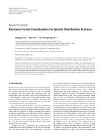
3.4. Effect of sample rate and size on
genre classification
When an audio file is compressed under different settings,
its features could change. In order to understand what
changes could happen, we used different sample rates
(22.050 kHz, 32 kHz, 44.1 kHz), sample sizes (8 bit, 16 bit) to
convert the audio file to wav format. As seen in Figure 1,we
examined the normalized mean difference between features
on all data points using one setting versus another setting.
302520151050
Marsyas features
2
1.5
1
0.5
0
0.5

1
1.5
Normalized mean difference
Mean(x
32,8
x
22,8
)/std(x
32,8
)
Mean(x
32,8
x
44,8
)/std(x
32,8
)
Mean(x
32,8
x
32,16
)/std(x
32,8
)
Figure 1: The change of Marsyas features when different sample
rates and sample sizes are used.
There is some variability on all the features, although fea-
tures 6 (BEAT), 7, 8 and 10 (STFT) seem to vary more than
others.
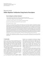
In order to understand the effect of feature changes due

to compression settings, we trained different classifiers using
different feature sets (ALL, BEAT, MFCC, MPITCH, STFT)
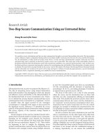
obtained under different compression settings. In Figures 2
and 3, the x-axis shows different audio sampling rates and
sizes: 1 : 22.05 kHz, 8 bit; 2 : 22.05 kHz, 16 bit; 3 : 32 kHz,
8bit;4:32kHz,16bit;5:44.1 kHz, 8 bit, 6 : 44.1kHz,16bit.
For each genre, 90% of all available data was used for training
and 10% was used for testing. In the figures and tables below,
the test classification accuracies are reported. Using ALL fea-
tures almost always gave better performance than using one
of the other specified feature sets. MFCC’s performance was
very close to that of ALL, though. MPITCH and BEAT usu-
ally gave the least classification accuracy. When ALL features
were used, we found out that the expected perfor mance did
not change a lot between different sample rates and sizes.
Table 1 shows the root and leaf genre classification ac-
curacies obtained using the first and last two (22.05 kHz or
44.1 kHz and 8 or 16 bits) compression settings. LDC per-
forms better than 10 NN for both root and genre classifica-
tion.
4. GENRE CLASSIFICATION USING MIDI AND NCD
One way to measure the distance between two music pieces
is to first extract features and then measure distance between
feature vectors. For example, [4] uses 109 features of musical
information such as orchestration, number of instruments,
adjacent fifths, and so forth. Once distances are available, a
classification algorithm, such as k-nearest neighbor, can be
used to predict the genre of a music piece.
4 EURASIP Journal on Advances in Signal Processing
654321

Audio sampling rates and sizes
0
10
20
30
40
50
60
70
80
90
100
Classification performance
ALL
BEAT
MFCC
MPITCH
STFT
Figure 2: Root genre test classification accuracies of LDC classifier
using different sets of features (each curve) at different audio sam-
pling rates and sizes (x-axis).
654321
Audio sampling rates and sizes
0
10
20
30
40
50
60

70
80
90
100
Classification performance
ALL
BEAT
MFCC
MPITCH
STFT
Figure 3: Leaf genre test classification accuracies of LDC classifier
using different sets of features (each curve) at different audio sam-
pling rates and sizes (x-axis).
In this study, in order to measure the distance between
two music pieces, we use normalized compression distance
(NCD). According to NCD, two objects are said to be close if
the information contained in one of them can be compressed
in the other. In other words, if t wo pieces are similar, then it is
possible to describe one given the other. The compression is
based on the ideal mathematical notion of Kolmogorov com-
plexity, which unfortunately is not effectively computable.
Table 1: Root and leaf genre test classification accuracies on audio
data obtained from MIDI, using different compression settings and
10 NN and LDC classifiers.
Audio
22.05 kHz,
8bits(1)
22.05 kHz,
16 bits (2)
44 kHz,

8bits(5)
44 kHz,
16 bits(6)
Root, 10 NN 0.52 ± 0.01 0.53 ± 0.01 0.54 ± 0.01 0.58 ± 0.01
Root, LDC
0.86 ± 0.01 0.84 ± 0.01 0.83 ± 0.01 0.86 ± 0.01
Leaf, 10 NN
0.19 ± 0.01 0.20 ± 0.01 0.23 ± 0.01 0.30 ± 0.01
Leaf, LDC
0.59 ± 0.01 0.63 ± 0.01 0.60 ± 0.01 0.63 ± 0.01
Table 2: Root and leaf genre test classification accuracies on MIDI
data using 10 NN classifier with NCD.
MIDI 30 seconds 60 seconds 120 seconds ALL
Root 0.67 ± 0.01 0.66 ± 0.01 0.67 ± 0.01 0.75 ± 0.01
Leaf
0.31 ± 0.01 0.39 ± 0.01 0.46 ± 0.01 0.42 ± 0.01
However, it is possible to approximate the Kolmogorov com-
plexity by using standard compression techniques. NCD uses
no background knowledge about music, it is completely gen-
eral and can, without change, be used in different areas like
linguistic classification and genomics.
In [6, 7], first the MIDI representation of a music piece is
processed and transformed into a string from a finite alpha-
bet. Then the distance between two music pieces x and y are
computed using their NCD:
d(x, y)
=
max

K(x | y), K(y | x)


max

K(x), K(y)

. (1)
In this formula, K(x) denotes the Kolmogorov complexity
of x and K(x
|y) denotes the Kolmogorov complexity of x
given y. K(x
|y) is approximated using K(x|y) ≈ K(xy) −
K(x). NCD uses the compressed length of a string as an ap-
proximation of its Kolmogorov Complexity. K(xy)iscom-
puted simply as the compressed length of x and y concate-
nated together. This compressed length approximation to
Kolmogorov complexity seems to have given good results for
anumberofdifferent data sets in [8].
In this study, we use our preprocessor [16, 17]onMIDI
files to turn them into strings. The MIDI preprocessor sam-
ples the MIDI file at each 5 ms. and discovers the notes simul-
taneously played at each interval. It converts each note played
in that interval to an integer between 0 and 127. Since all
pieces used in experiments are polyphonic, like in most of the
cases in the real world, polyphonic to monophonic conver-
sion is needed. The note which is heard as the highest pitch
[23] is taken as the representative of the interval. Then the
difference between consecutive monophonic notes is taken
and written to a binary file. Apart from [6, 7], tempo varia-
tions are taken into account and difference between consec-
utive monophonic notes is taken. Like them, we use NCD as

the distance measure between two pieces.
Table 2 shows the root and leaf genre classification ac-
curacy of the 10 NN classifier using NCD as the distance
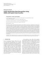
Zehra Cataltepe et al. 5
MIDI representation
of a music pieces s
x
x
training data
MIDI-to str. MIDI-to str. MIDI-to audio
NCD Marsyas
d(x, x
) x audio features of s
pm
= outputs of classifiers trained
according to d(x, x
)
pa
= outputs of classifiers trained
using training data
Weighted majority voting
Label of s
Figure 4: A method to combine MIDI and audio features to predict the genre of a MIDI music piece.
measure. Distances are computed using the first 30, 60,
120 seconds and finally using all the available music piece.
The accuracies shown are computed over 100 different
train/test partitions of all the available data. Using the whole
piece results in the best root genre classification perfor mance,
while using only the first 120 seconds results in the best leaf
genre classification perfor m ance. Note that, as in the case of

the previous section, the root and leaf genre classification
performances are quite below the results obtained in [4].
5. GENRE CLASSIFICATION USING BOTH
MIDI AND AUDIO FROM MIDI
We explored the root and leaf genre classification accuracy
using MIDI and audio separately and found out that the ac-
curacy varied between different feature sets and classifiers.
However, the accuracies reached were far below the accura-
cies obtained in [4]. In this section, we investigate if we can
get better results by combining MIDI and audio classifiers we
obtained in the previous two sections.
According to Kuncheva [24], in order for classifier com-
bination to be successful, classifiers need to be diverse. The
probability that many classifiers, trained independently, will
agree on the same wrong output is small. Therefore, majority
voting could give the right answer for the many, independent
and diverse classifiers case.
There are a number of methods to achieve diverse classi-
fiers: (a) use independent sub samples of data to train each
classifier, (b) use different sets of features to train each clas-
sifier, (c) use different algorithms to train each classifier. In
this paper, we use (b) and (c) to achieve classifier diversity.
MIDI distances and audio features give us an initial base
of different features. We get still more different features by
using different initial portions of the MIDI file and differ-
ent sample rates and sizes for the audio file. The k-nearest
neighbor and LDC classifiers also help achieve more diver-
sity. Therefore, we have a pool of different classifiers whose
voteswecancombinetoachievebetteraccuracy(Figure 4).
Let D

i
, i = 1, , L, indicate the different trained clas-
sifiers. In this paper, L
= 12 and i = 1 : 4 correspond
to 10 NN classifiers, trained using NCD between MIDI files.
i
= 5 : 8 corresponds to 10 NN classifiers, trained using all 30
features. i
= 9 : 12 corresponds to linear discriminant classi-
fiers trained, again, using all 30 features. Let d
i, j
be 1 if clas-
sifier i labels x in class j and 0 otherwise. Let w
i
denote the
weight of classifier i. The weighted majority voting chooses
class j
∗
such that
j
∗
= arg max
j=1, ,L

i=1, ,C
w
i
d
i, j
. (2)

We consider four different flavors of weighted majority vot-
ing described by the weights w
i
given to each classifier.
6 EURASIP Journal on Advances in Signal Processing
Table 3: Root and leaf genre classification accuracies when classifiers are combined.
MIDI
w
i
= 1
i
= 1 − 4:w
i
= 2
w
i
α acc
i
w
i
optimal
and
i = 5 − 8:w
i
= 1
audio
i = 9 − 12 : w
i
= 2
Root 0.88 ± 0.01 0.89 ± 0.01 0.89 ± 0.01 0.93 ± 0.01

Leaf
0.58 ± 0.01 0.58 ± 0.01 0.58 ± 0.01 0.62 ± 0.01
Table 4: Root genre confusion matrices for 12 different base classifiers.
No Feature, classifier
Actual = classic Actual = jazz Actual = pop
Pred class Pred jazz Pred pop Pred class Pred jazz Pred pop Pred class Pred jazz Pred pop
1 MIDI, 30 s, 10 NN 89 7 4 14 82 4 45 26 29
2
MIDI, 60 s, 10 NN 69 13 18 686 825 33 42
3
MIDI, 120 s, 10 NN 70 4 26 8761620 23 56
4
MIDI, ALL, 10 NN 75 4 21 6841013 22 66
5
Audio, 22, 8, 10 NN 72 13 15 10 48 41 21 42 37
6
Audio, 22, 16, 10 NN 71 6 23 12 41 47 19 34 47
7
Audio, 44, 8, 10 NN 63 15 22 8533914 39 47
8
Audio, 44, 16, 10 NN 69 12 19 14 46 40 10 30 60
9
Audio, 22, 8, LDC 94 3 2 688 612 13 75
10
Audio, 22, 16, LDC 96 0 4 3871012 20 68
11
Audio, 44, 8, LDC 98 1 2 28216 92170
12
Audio, 44, 16, LDC 97 0 3 48214 41878
(i) w

i
= 1: this voting scheme gives each classifier the
same amount of vote.
(ii) w
i
= 2if1 ≤ i ≤ 4or9 ≤ i ≤ 12 and w
i
= 1if
5
≤ i ≤ 8: inspired by the fact that audio-10 NN gives
the worst results, this method gives less weight to those
classifiers.
(iii) w
i
proportial to accuracy of ith classifier: this method
depends on the accuracy of each classifier which is not
available. However, using a subset of training data for
validation accuracy could be estimated.
(iv) w
i
selected to maximize accuracy: this method exhaus-
tively searches the w
i
’s in [0.2 : 1] interval and reports
the w
i
that results in the best accuracy. This method
is also not realizable in practice, however, it is included
to report the best possible performance using weighted
majority voting.

Table 3 shows the leaf and root genre classification accuracies
of each classifier combination method. Comparison of Tables
1, 2,and3 shows that root genre classification accuracy in-
creases when classes are combined for all of the combination
schemes.
Table 4 shows the confusion matrix entries for each of the
base classifiers. The entries are averaged over 100 train/test
partitions and normalized to 100 per actual class. Each row
corresponds to a classifier with a different feature and clas-
sification method. Second column shows whether the MIDI
or audio input is used and the type of classifier used. This
column also shows the length of the used piece for MIDI and
the sample rate and sample size for audio. Although the ac-
curacies were similar, clearly the confusion matrices are dif-
ferent for each feature-classifier combination and this helped
combination achieve better results. Another observation is
that classic is recognized best when 30 seconds of MIDI file
is used, whereas pop benefits from longer files. While higher
quality (i.e., more kHz and 16 bits) encoding usually helps
classic and pop, the same is not true for jazz.
Table 5 shows the confusion matrices for the classifier
combinations. Using audio and LDC usually gave the best
results on Tabl e 4,andTabl e 5’s entries are better than that.
Choosing classifier weights according to accuracies did not
improve over the equal-weighted majority voting. On the
other hand, choosing the optimal weights according the spe-
cific set of samples being classified resulted in better perfor-
mance.
6. CONCLUSIONS
In this paper, we first classified genres using MIDI files us-

ing normalized compression distance (NCD) and 10-nearest
neighbor (10 NN) classifier. We converted MIDI files to au-
dio and did genre classification using features at different
sample rates and sizes and LDC and KNN classifiers. Finally,
we combined 12 different classifiers we obtained at the pre-
vious steps, using different schemes of majority voting. We
found out that majority voting improved the classification
accuracy. The classification accuracies for MIDI or audio
only were much below the results obtained in [4]. Classifier
combination improved genre classification, althoug h the re-
sults are still worse than those reported by [4] on their data
sets. Since 109 different domain-based features such as or-
chestration, number of instruments, adjacent fifths, and so
Zehra Cataltepe et al. 7
Table 5: Root genre confusion matrices for four different combinations of base classifiers.
Actual = classic Actual = jazz Actual = pop
Combination method Pred class Pred jazz Pred pop Pred class Pred jazz Pred pop Pred class Pred jazz Pred pop
w
i
= 1 99 0 1 3934 81972
i
= 1 − 4:w
i
= 2
99 0 1 3934 81776
i
= 5 − 8:w
i
= 1
i = 9 − 12 : w

i
= 2
w
i
α acc
i
99 0 1 3934 81776
w
i
optimal 100 0 0 2943 51086
forth were used in [4], and, for example, instrumentation
features were assigned up to 42% weight among their fea-
tures, we think that our results could be improved if instead
of using NCD, we used features similar to those reported in
[4]. We should also note that, in contrast to [4], the approach
outlined in this paper does not require any musical back-
ground knowledge.
Currently, the audio to MIDI conversion is not very suc-
cessful, especially when multiple instruments are used in
the piece. We hope that as technology gets better, a similar
approach that combines audio and audio-to-MIDI features
could be used to improve audio genre classification.
ACKNOWLEDGMENTS
We would like to express our gr atitude to George Tzanetakis
and Cory McKay for generously sharing their data sets. We
also would like to thank Tzanetakis for Marsyas, Cilibrasi,
and colleagues for Complearn and Bob Duin and colleagues
for PrTools, which was used in some of the exper iments. We
thank the reviewers for helping us improve the quality of the
paper.

REFERENCES
[1] S. Lippens, J. P. Martens, and T. De Mulder, “A comparison
of human and automatic musical genre classification,” in Pro-
ceedings of IEEE International Conference on Acoustics, Speech
and Signal Processing (ICASSP ’04), vol. 4, pp. 233–236, Mon-
treal, Quebec, Canada, May 2004.
[2] R. Basili, A. Serafini, and A. Stellato, “Classification of musical
genre: a machine learning approach,” in Proceedings of the 5th
International Conference on Music Information Retrieval (IS-
MIR ’04), Barcelona, Spain, October 2004.
[3] T. Jarvinen, P. Toiviainen, and J. Louhivuori, “Classification
and categorization of musical styles with statistical analysis
and self-organizing maps,” in Proceedings of the AISB Sympo-
sium on Musical Creativity, pp. 54–57, Edinburgh, Scotland,
April 1999.
[4] C. McKay and I. Fujinaga, “Automatic genre classification us-
ing large high-level musical feature sets,” in Proceedings of 5th
International Conference on Music Information Retrieval (IS-
MIR ’04), Barcelona, Spain, October 2004.
[5] G. Tzanetakis, A. Ermolinskyi, and P. Cook, “Pitch histograms
in audio and symbolic music information retrieval,” Journal of
New Music Research, vol. 32, no. 2, pp. 143–152, 2003.
[6]R.Cilibrasi,P.M.B.Vit
´
anyi, and R. de Wolf, “Algorithmic
clustering of music based on string compression,” Computer
Music Journal, vol. 28, no. 4, pp. 49–67, 2004.
[7] M. Li, X. Chen, X. Li, B. Ma, and P. M. B. Vit
´
anyi, “The similar-

ity metric,” IEEE Transactions on Information Theory, vol. 50,
no. 12, pp. 3250–3264, 2004.
[8] E. Keogh, S. Lonardi, and C. A. Rtanamahatana, “Towards
parameter-free data mining,” in Proceedings of the 10th ACM
SIGKDD International Conference on Knowledge Discovery and
Data Mining (KDD ’04), pp. 206–215, Seattle, Wash, USA, Au-
gust 2004.
[9] D. Pan, “A tutorial on MPEG/audio compression,” IEEE Mul-
timedia, vol. 2, no. 2, pp. 60–74, 1995.
[10] J. J. Aucouturier and F. Pachet, “Representing musical genre: a
state of the art,” Journal of New Music Research, vol. 32, no. 1,
pp. 83–93, 2003.
[11] T. Lidy and A. Rauber, “Evaluation of feature extractors and
psycho-acoustic transformations for music genre classifica-
tion,” in Proceedings of the 6th International Conference on Mu-
sic Information Retrieval (ISMIR ’05),London,UK,September
2005.
[12] G. Tzanetakis and P. Cook, “Musical genre classification of au-
dio signals,” IEEE Transactions on Speech and Audio Processing,
vol. 10, no. 5, pp. 293–302, 2002.
[13] C. Xu, N. C. Maddage, X. Shao, F. Cao, and Q. Tian, “Musi-
cal genre classification using support vector machines,” in Pro-
ceedings of IEEE International Conference on Acoustics, Speech
and Signal Processing (ICASSP ’03), vol. 5, pp. 429–432, Hong
Kong, April 2003.
[14] F. Gouyon, S. Dixon, E. Pampalk, and G. Widmer, “Evaluat-
ing rhythmic descriptors for musical genre classification,” in
Proceedings of the 25th International AES Conference,London,
UK, June 2004.
[15] K. West and S. Cox, “Features and classifiers for the automatic

classification of musical audio sig nals,” in Proceedings of the
5th International Conference on Music Information Retrieval
(ISMIR ’04), Barcelona, Spain, October 2004.
[16] A. Sonmez, “Music genre and composer identification by u s-
ing Kolmogorov distance,” M. Sc. thesis, Computer Engineer-
ing Department, Istanbul Technical University, Istanbul, Tur-
key, 2005.
[17] Z. Cataltepe, A. Sonmez, and E. Adali, “Music classification us-
ing Kolmogorov distance,” in Representation in Music/Musical
Representation Congress, Istanbul, Turkey, October 2005.
[18] T. Li, M. Ogihara, and Q. Li, “A comparative study on content-
based music genre classification,” in Proceedings of the 26th An-
nual International ACM SIGIR Conference on Research and De-
velopment in Information Retrieval (SIGIR ’03), pp. 282–289,
Toronto, Ontario, Canada, July-August 2003.
8 EURASIP Journal on Advances in Signal Processing
[19] D. Turnbull and C. Elkan, “Fast recognition of musical gen-
res using RBF networks,” IEEE Transactions on Knowledge and
Data Engineering, vol. 17, no. 4, pp. 580–584, 2005.
[20] R.O.Duda,P.E.Hart,andD.G.Stork,Pattern Classification,
John Wiley & Sons, New York, NY, USA, 2000.
[21] J. Bergstra, N. Casagrande, and D. Eck, “Genre classification:
timbre and rhythm-based multiresolution audio classifica-
tion,” in Proceedings of 1st Annual Music Information Retrieval
Evaluation eXchange (MIREX) Genre Classification Contest,
London, UK, September 2005.
[22] T. Li and G. Tzanetakis, “Factors in automatic musical genre
classification of audio signals,” in Proceedings of IEEE Work-
shop on Applications of Signal Processing to Audio and Acoustics
(WASPAA ’03), New Paltz, NY, USA, October 2003.

[23] L. Uitdenbogerd and J. Zobel, “Music ranking techniques eval-
uated,” Australian Computer Science Communications, vol. 24,
no. 1, pp. 275–283, 2002.
[24] L. I. Kuncheva, Combining Pattern Classifiers, John Wiley &
Sons, New York, NY, USA, 2004.
Zehra Cataltepe is an Assistant Professor at
Computer Engineering Department, Istan-
bul Technical University. Her research inter-
ests are machine learning theory and appli-
cations, especially in bioinformatics, web/
document mining, and music recognition
and recommendation. She got her Ph.D. de-
gree from Caltech in computer science in
1998 and her B.S. degree from Bilk-ent Uni-
versity, Ankara, in 1992. She worked at Bell
Labs as a postdoc and then at StreamCenter Inc. and Siemens Cor-
porate Research as researcher after she got her Ph.D.
Yusuf Yaslan received the B.S. degree in
computer science engineering from Istan-
bul University, Turkey, in 2001. During
2001 and 2002, he was a practical trainer
at the FGAN-FOM Research Institute, in
Germany. In 2002, he joined the Multime-
dia Signal Processing and Pattern Recogni-
tion laboratory at Istanbul Technical Uni-
versity (ITU). He received his M.S. degree in
telecommunication engineering from ITU,
Turkey, in 2004. He is currently working at Computer Engineer-
ing Department at ITU as a research assistant, and pursuing his
Ph.D. in the same department. His research interests are in pattern

recognition, data and web mining, audio watermarking, and music
recommendation.
Abdullah Sonmez is a Ph.D. candidate at
the Department of Computer Engineering
at Istanbul Technical University and cur-
rently working in R&D center of Teknobil
Inc. as a researcher and developer. His re-
search interests include information retrival
especially in music, data mining and ma-
chine learning, especially in bioinformat-
ics, GSM and satellite-based communica-
tion networks and VoIP. He got his M.S. de-
gree from Istanbul Technical University in computer engineering
in 2005 and his B.S. degree from Istanbul Technical University in
2002.