Báo cáo hóa học: " Research Article Applying Novel Time-Frequency Moments Singular Value Decomposition Method and Artificial Neural Networks for Ballistocardiography" docx

Hindawi Publishing Corporation
EURASIP Journal on Advances in Signal Processing
Volume 2007, Article ID 60576, 9 pages
doi:10.1155/2007/60576
Research Article
Applying Novel Time-Frequency Moments Singular
Value Decomposition Method and Artificial Neural
Networks for Ballistocardiography
Alireza Akhbardeh,
1
Sakari Junnila,
1
Mikko Koivuluoma,
1
Teemu Koivistoinen,
2
and Alpo V
¨
arri
1
1
Institute of Signal processing, Tampere University of Technology, Korkeakoulunkatu 1, 33101 Tampere, Finland
2
Department of Clinical Physiology and Nuclear Medicine, Tampere University Hospital, Teiskontie 35,
33521 Tampere, Finland
Received 8 April 2005; Revised 5 April 2006; Accepted 10 September 2006
Recommended by Bernard Mulgrew
As we know, singular value decomposition (SVD) is designed for computing singular values (SVs) of a matrix. Then, if it is used
for finding SVs of an m-by-1 or 1-by-m array with elements representing samples of a signal, it will return only one singular
value t hat is not enough to express the whole signal. To overcome this problem, we designed a new kind of the feature extraction
method which we call “time-frequency moments singular value decomposition (TFM-SVD).” In this new method, we use statistical

features of time series as well as frequency series (Fourier transform of the signal). This information is then extracted into a certain
matrix with a fixed structure and the SVs of that matrix are sought. This transform can be used as a preprocessing stage in pattern
clustering methods. The results in using it indicate that the performance of a combined system including this transform and
classifiers is comparable with the performance of using other feature extraction methods such as wavelet transforms. To evaluate
TFM-SVD, we applied this new method and artificial neural networks (ANNs) for ballistocardiogram (BCG) data clustering to
look for probable heart disease of six test subjects. BCG from the test subjects was recorded using a chair-like ballistocardiograph,
developed in our project. This kind of device combined with automated recording and analysis would be suitable for use in many
places, such as home, office, and so forth. The results show that the method has hig h performance and it is almost insensitive to
BCG waveform latency or nonlinear disturbance.
Copyright © 2007 Alireza Akhbardeh et al. This is an open access article distributed under the Creative Commons Attribution
License, which permits unrestr icted use, distr ibution, and reproduction in any medium, provided the original work is properly
cited.
1. INTRODUCTION
Ballistocardiogram (BCG) [1, 2] is a movement-related sig-
nal caused by shifts in the center of the mass of the blood,
which consists of components attributable to cardiac activ-
ity, respiration, and body movements. One of the advantages
of the BCG measurement is that no electrodes are needed
to be attached to the subject [3]. Therefore, it could provide
the possibility of serving as a relatively low-cost, noninva-
sive, easy-to-use, home screening procedure for cardiac per-
formance assessment. Also, the BCG provides complimen-
tary information to traditional ECG measurements, telling
us more about the mechanical properties of the heart. An
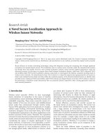
example of the BCG signal is shown in Figure 1 [4]. Dur-
ing the past several years, some classical as well as intelligent
pattern recognition methods have been developed for BCG
analysis. Yu and Dent [3] and Jansen et al. [5]listedsomeof
these methods in more detail. The performance of some of
the existing methods is very good when not considering elec-

tromechanical drifts, BCG cycle’s latency, motion artifac ts,
or other kinds of nonlinear disturbances [6]. The results will
have some errors if such important factors are not counted.
Another important limitation of the existing approaches is
their suitability for fast implementation as well as online pro-
cessing.
In this paper, we introduce a new method for feature
extraction, which we call “time-frequency moments singu-
lar value decomposition (TFM-SVD).” To evaluate the abil-
ity of the new method, we used it to compute the most im-
portant BCG waveform features and then clustered them
using an artificial neural network (ANN). To find the per-
formance of the combined approach, six test subjects from
three groups were used: two healthy young persons, two
healthy old men, and two old men with a previous heart
2 EURASIP Journal on Advances in Signal Processing
40
20
0
20
40
60
Amplitude
703 704 705 706 707 708 709 710
Time (s)
J
J
J
J
JJ

I
I
I
I
I
I
Figure 1: The heart-originated BCG signal during one respiratory
cycle [4]. The “I” and “J” spikes are marked with circles. The dot-
ted lines point the “R” spikes detected from the ECG signal, and
the dashed lines point the beginning and the end of the respiratory
cycle.
(myocardial) infarction. In Section 2, the used measurement
system is presented. The developed signal processing meth-
ods are presented in Section 3, followed by results and dis-
cussion.
2. MEASUREMENT SYSTEM
In the past, the BCG has been measured using several dif-
ferent methods. The most traditional way is to allow free
body movements in a supine (lying) position and to mea-
sure the body movements in the horizontal direction (head-
to-toe axis). In our work, we use pressure sensitive EMFi
1
sensors [7, 8] to measure small forces generated by the body
in a sitting position. For this purpose, a special measurement
chair fitted with EMFi-sensors under the upholstery was con-
structed [9]. Two sensor films were used, one for the seat
and one for the backrest. In this paper, we only use the sig-
nal recorded from the seat sensor. The charge signal from the
EMFi-sensors is converted to a voltage signal using a small-
charge amplifier. The converted signal was recorded together

with electrocardiogram (ECG), the impedance cardiogram
(ICG), and some other biosignals using a commercial Circ-
Mon (JR Medical Ltd, Tallinn, Estonia) circulation monitor
with a sampling frequency of 200 Hz. The sampling rate is
fixed in CircMon, but according to Shannon theorem and
BCG bandwidth, the sampling rate of 200 Hz is adequate, it
is about five times higher than BCG bandwidth (0–40 Hz)
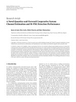
[10]. The chair and other devices of the system can be seen
in Figure 2. More information about the use of EMFi-sensors
for BCG measurement and the performance of the measure-
ment system can be found from publications [4, 11].
1
EMFi is a registered trademark of Emfit Ltd.
Figure 2: A chair equipped with an EMFi-film sensor, the charge
amplifier, a CircMon device, and a laptop PC.
Another similar BCG measurement technique is the
static-charge sensitive bed (SCSB). Its structure and opera-
tion are more complex, as it measures the “rubbing” action
applied to the film. Due to its str ucture, SCSB is more capa-
ble in detecting movement also parallel to the film plane [12].
The EMFi sensor is closer to a traditional force sensor, which
measures the force applied vertical to the film [13]. Accord-
ing to our experience, the signals measured from a supine
subject have similar temporal and spectral properties, but the
results are not the same. Therefore, in this application, with
measurements carried out in a sitting position and with the
sensor directly under the subject’s body, the EMFi-sensor is
well suited.
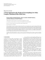
2.1. Patient recordings
BCG of the test subjects was recorded in a clinical tr ial at

Tampere University Hospital in 2004-2005 using the mea-
surement hardware presented in this section. A reference
ECG signal was recorded simultaneously from the chest of
the subject’s body. Examples of the recorded BCG/ECG sig-
nals are presented in Figure 3.
3. SIGNAL ANALYSIS PROCEDURES
Signal processing methods were applied to the data after the
recordings. The procedure we used for post-recording classi-
fication (Figure 4) of the recorded BCG data includes these
three steps: (A) BCG cycle extraction using the ECG signal
of the subject (segmentation stage); (B) feature computing
using TFM-SVD; (C) using ANNs to cluster features. These
stages are discussed in detail in the following subsections.
3.1. BCG data segmentation
The final aim of this research work is the BCG cycle cluster-
ing, not BCG data segmentation. In this work, we used the
ECG data of the subjects to extract BCG waveforms in every
Alireza Akhbardeh et al. 3
5
4
3
2
1
0
1
2
3
4
5
ECG

20 21 22 23 24 25 26 27 28
Time (s)
(a)
5
4
3
2
1
0
1
2
3
4
5
BCG
20 21 22 23 24 25 26 27 28
Time (s)
(b)
Figure 3: Typical ECG and BCG records of a normal subject.
cardiac period. To achieve this aim, the R-components of
the ECG signal, threshold detecting, and 250 point windows
were used. The raw signal from the EMFi-sensor includes
components of breathing, motion artifacts, low and high fre-
quency noises, and so forth. Thus, we had to use a bandpass
filter to extrac t the heart-originated BCG signal. According
to our experience, if we use a bandpass filter of [3, 14]Hzto
smooth the recorded BCG signals, we can extra ct the most
important components of BCG signals for pattern recogni-
tion purposes, and remove other components. Of course, for
monitoring or other purposes, we must use another type of

filtering, but for our application this bandwidth was found
suitable.
3.2. BCG features extraction using TFM-SVD
To define T FM-SVD, first we must be familiar with singular
value decomposition (SVD), briefly explained below.
3.2.1. Singular value decomposition
Singular value decomposition is used because it captures the
essential information of a matrix, somewhat similarly as the
eigenvalues do. A singular value and the corresponding sin-
gular vectors of a rectangular matrix A are a scalar σ and a
pair of vectors u and v that satisfy
Aν
= σu,
A
T
u = σν.
(1)
With the singular values on the diagonal of a diagonal matrix
and the corresponding singular vectors forming the columns
Recorded
BCG signal
Recorded
ECG signal
BCG cycles extraction
using R-component of ECG
Time-frequency moments
singular value decomposition
Neural networks
Youn g
normal

Old
normal
Old
abnormal
Figure 4: Block diagram of the post-recording signal analysis.
of two orthogonal matrices U and V,wehave
AV
= U

,
A
T
U = V

.
(2)
Since U and V are orthogonal, this becomes the singular
value decomposition
A
= U

V
T
. (3)
The full singular value decomposition of an m-by-n matrix
involves an m-by-mU,anm-by-n

,andann-by-nV.In
other words, U and V are both square and are the same size
as A.IfA has many more rows than columns, the resulting U

can be quite large, but most of its columns are multiplied by
zeros in

. In this situation, the economy sized decomposi-
tion saves both time and storage by producing an m-by-nU,
an n-by-n

, and the same V [15].
3.2.2. Time-frequency moments singular
value decomposition
As explained in the previous section, the singular value de-
composition (SVD) is an appropriate tool for analyzing a
mapping from one vector space into another vector space,
possibly with a different dimension. If the matrix under anal-
ysis is square, symmetric, and positive definite, then its eigen-
value and singular value decompositions are the same. In
particular, the singular value decomposition of a real ma-
trix is always real, but the eigenvalue decomposition of a real
nonsymmetric matrix might be complex [15]. However, if
we use i t to find SVs o f an m-by-1or1-by-m array with el-
ements representing samples of a signal, it will return only
onesingularvaluethatisnotenoughtoexpressallpartsofa
signal.
To overcome this problem, we introduce a new kind
of feature extraction method the so-called time-frequency
4 EURASIP Journal on Advances in Signal Processing
moments singular value decomposition (TFM-SVD) in this
paper. In this new method, we suggest the use of eight sta-
tistical features of the input signal in time domain as well
as frequency domain. The reason for the use of both time

and frequency domains is that if the signal under analysis
is a nonstationary signal, as most biological sig nals and our
example BCG are, then we will need a time-frequency ana-
lyzing tool to find its most important features, and we can-
not use the transforms that use either temporal or frequency
features. Although there are some other existing transforms
such as the wavelet transform to analyze BCG [14, 16–18], we
tried to introduce another kind of BCG analysis w hich is able
to give results similar to results of the wavelet transform. Our
suggestion is to form two matrices: one to s tore the most el-
ementary statistical parameters of the signal in time domain
(Mt) and another one (Mf) to store the most elementary
statistical parameters of the frequency domain representa-
tion of the signal. After that, we can use singular value de-
compositions (SVD) to extract singular values (SVs) of those
matrices. We can use these obtained SVs as the most impor-
tant features of the input signal. The proposed method has
the following steps to compute eight features of s ignal “x[n]”
with length N (samples), which is inside the range [
5, 5].
(1) Run fast fourier transform (FFT) algorithm to find
spectrum (y[m]) of signal x[n].
(2) Compute four statistical moments of time-series x[n]
which are
mean
= E[x] = μ,
variance
t = E

(x μ)

2

,
sharpness
t = E

(x μ)
3

,
4th moment
t = E

(x μ)
4

.
(4)
(3) Compute statistical moments of frequency-series
y[m]:
mean
= E[y] = μf,
variance
f = E

(y μf)
2

,
sharpness

f = E

(y μf)
3

,
4th moment
f = E

(y μf)
4

.
(5)
(4) Assemble a new matrix (Mt) with the four following
statistical moments of the input signal in time domain
(x[n]):
Mt
=

a μ variance t/b
sharpness
t/c 4th moment t/d

,(6)
where a, b, c, d are constant values and must be in the
range where four elements of this matrix are scaled to
the range [L1, L2]. This scaling is needed to make all
elements of the matrix Mt uniform to the same range.
(5) Assemble another matrix (Mf) with the following

four statistical moments of the spectrum of the input
(y[m]):
Mf
=

af μf variance f/bf
sharpness
f/cf 4th moment f/df

,(7)
where, again, af, bf, cf, df are constant values and must
be in the range where four elements of the matrix Mf
are scaled to the range [L3, L4]. This scaling is needed
to make all elements of the matrix Mt uniform to the
same range.
(6) Find singular values (SVs) of the matrix Mt:SVD
(Mt); this will return two SVs for any kind of input sig-
nal x[n], because the dimension of Mt matrix is 2
2.
(7) Find singular values (SVs) of matrix Mf:SVD(Mf);
this will return another two SVs for any kind of spec-
trum (y[m]) of an input signal, because the dimension
of the Mf matrix is 2
2.
(8) Finally, assemble the so-called time-frequency mo-
ments (TFM) vector with dimension 4
1:
TFM matrix
=


SVD(Mt)
SVD(Mf)

. (8)
As can be seen, these steps will return fixed four SVs
of time-frequency moments for any type of signal with any
size. The properties of this new kind of the feature extraction
method are suitable especially for our application because we
would like to optimize and reduce the dimension of the in-
put s ignals (BCG cycles) as much as p ossible. This method is
quite insensitive to phase shifting of the BCG cycles because
of its structure.
The reason behind choosing the above-mentioned four
moments is their ability to extract essential information from
both time and frequency domains. In probability theory and
statistics, the mean is the expected value of a real-valued ran-
dom variable (signal x), which is also called the population
mean. For a data set, the mean is just the sum of all the obser-
vations divided by the number of observations. The variance
of a random variable is a measure of its statistical dispersion,
indicating how far from the expected value its values typically
are. The variance of a real-valued random variable is its sec-
ond central moment, and it also happens to be its second cu-
mulant. The variance of a random variable is the square of its
standard deviation. Sharpness shows the amplitude and the
direction of the changes in the random process. The four t h
moment, similar to Kurtosis, is a measure of the “peaked-
ness” of the probability distribution of a real-valued random
variable. Higher fourth moment means that more of the vari-
ance is due to infrequent extreme deviations, as opposed to

frequent modestly sized deviations. The other four features
indicate the same measures that form the frequency domain
of a real-valued random variable. In our tests, we found that
higher than four moments do not give us new information
compared to moments one to four. Although we recommend
only using the first four moments of a real-valued random
variable in the proposed algorithm, it is possible to add more
moments, in both time and frequency domains, to the above-
mentioned algorithm.
Alireza Akhbardeh et al. 5
Singular value decomposition is used because it captures
the essential information of a matrix (compression), some-
what similarly as the eigenvalues do. Referring to our expe-
riences, using SVD after the extraction of the moments gives
us better ability to train a neural network for pattern classifi-
cation.
The choice of TFM normalization parameters depends
on the input signal range. For instance, if the input signal
is inside the range [α
1
, α
2
]whereα
2
>α
1
, the time domain
moments will be in these ranges:
α
1

μ α
2
,
0
variance t

α
2
α
1

2
,

α
2
α
1

3
sharpness t

α
2
α
1

3
,
0

4th moment t

α
2
α
1

4
.
(9)
So, the constant values of time domain must be
a
=
α
2
α
1
max



α
1


,


α
2




,
b
= α
2
α
1
,
c
=

α
2
α
1

2
,
d
=

α
2
α
1

3
(10)

to have an Mt matrix in the range

L1 =

α
2
α
1

, L2 = +

α
2
α
1

. (11)
The moments in the frequency domain will be in these
ranges:
N
α
1
μ
f
N α
2
,
0
variance f N
2


α
2
α
1

2
,
N
3

α
2
α
1

3
sharpness f N
3

α
2
α
1

3
,
0
4th moment f N
4


α
2
α
1

4
,
(12)
where N is the length of the signal. Thus, the constant values
of frequency domain must be
af
=
α
2
α
1
N max



α
1


,


α
2




,
bf
= N
2

α
2
α
1

,
cf
= N
3

α
2
α
1

2
,
df
= N
4

α

2
α
1

3
(13)
to have an Mf matrix in the range

L3 =

α
2
α
1

, L4 = +

α
2
α
1

. (14)
3.2.3. BCG feature computing using TFM-SVD
In this study, we used TFM-SVD and computed TFM-SVs
of every BCG cycle x[n] using the procedure explained in
Section 3.2.2. Every BCG cycle has 250 samples because of
our measurement system and its sampling rate (200 HZ).
The TFM-SVD method helps us to find the most impor-
tant features of the BCG cycles (waveforms) and to reduce

the cycle’s dimension (N)fromN
= 250 features to 4 fea-
tures. Before using the TFM-SVD algorithm, we must ini-
tialize its constant values. In this study, we used N
= 250,
L1
= L3 = 10, and L2 = L4 = 10, so constants are
a
= 2, b = 10, c = 100, d = 1000, af = 2/250, bf =
250
2
10 = 6.25 10
5
,cf = 250
3
10
2
= 1.5625 10
9
,
df
= 250
4
10
3
= 3.90625 10
12
. On the other hand, they
shift Mt and Mf elements’ values to the range [
10, 10] if

the input signal’s values (x[n]) are inside the range [
5, 5].
This range (L1
= L3 = 10, and L2 = L4 = 10) is chosen for
convenience and there are no restrictions on initializing the
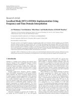
TFM-SVD constants. The results (TFM-SV features of whole
extracted BCG cycles) in a 3D presentation for six typical
subjects (two young normal, two old normal, and two old
abnormal subjects) are shown in Figure 5. As we explained,
the TFM-SVD algorithm returns only four features for every
BCG cycle. To show how these features are scattered in a 3D
presentation, we have to consider only the first three features
and ignore the fourth one for every BCG cycle.
3.3. BCG data clustering using artificial
neural networks
For BCG feature classification, we used two kinds of very fa-
mous ANNs: multilayer perceptrons (MLPs) and radial basis
functions (RBFs) [19, 20]. Before presenting the TFM-SVD
and the coefficients of the BCG cycles to the neural network,
we must normalize them to the range [0,1].
3.3.1. Multilayer perceptrons
M ultilayer perceptrons (MLPs) are feed-forward neural net-
works trained with the standard back propagation algorithm.
They are supervised networks, which means that they require
a desired response in order to be trained. They lear n how to
transform input data into a desired response, and therefore
they are widely used for pattern classification. With one or
two hidden layers, they can approximate virtually any input-
output map. They have been shown to approximate the per-
formance of optimal statistical classifiers in difficult prob-

lems. Most neural network applications involve MLPs.
3.3.2. Radial basis functions
RBF networks [19, 20] employ neurons that consist of radial
basis functions. In contrast to classic multilayer perceptrons,
the activation of a neuron is not given by the weighted sum
6 EURASIP Journal on Advances in Signal Processing
0
0.2
0.4
0.6
0.8
Singular value 1
(frequency domain)
0
0.2
0.4
0.6
0.8
1
Singular value 1 (time domain)
1
0.8
0.6
0.4
0.2
0
Singular value 2
(time domain)
Young healthy
Old healthy

Old unhealthy
3D BCG time-frequency singular
values (TFSVs) distribution
Figure 5: A 3D scattergram for TFM-SV features of all extr acted BCG cycles of six subjects under test (two young normal, two old normal,
and two old abnormal subjects). Only the first three features of the TFM-SVD algorithm are normalized to [0,1] and shown in this 3D
visualization.
of all its inputs but by the computation of a radial basis func-
tion. Generally, the kernels-Gaussian function
ϕ(u; t
k
) = exp

1
σ
2
k


u t
k


2

, k = 1, 2, , k, σ
k
> 0,
(15)
is used where u is the input of the neuron, t is the basis of the
neuron, and σ is the amplitude of the neuron. RBF networks

are feed-forward networks and consist of one input layer (u),
one hidden layer of Gaussian neurons (H), and one output
layer (y). The value of an output unit y
i
(given a network
input u)iscomputedby
y
i
=
K

k=1
w
ik
ϕ
i

u; t
k

+ w
i0
, (16)
where w
ik
is the weight (= height) of neuron Hi for output y
i
and w
i0
is a general threshold (bias) of output y

i
subtracted
from the weighted inputs. The Gaussian neurons work as ex-
perts for certain areas of the d-dimensional input space. Ac-
tivation of each neuron depends on its distance to the input
vector. Learning algorithms like back propagation (we used a
stochastic learning [9, 10]) can be used to adjust the nonfixed
parameters of the network including kernels centers, weights,
and stigma.
4. RESULTS
To demonstrate the performance of our approaches and to
compare results, we used MLP (two hidden layers with 15
and 10 neurons relatively) and RBF neural networks (hidden
layer with 15 neurons) with 4 inputs, and 3 outputs to clas-
sify 6 subjects into 3 categories: young healthy students aged
between 20–30 years (2 subjec ts), old healthy men aged be-
tween 50–70 years (2 subjects), and two old subjects (50–70
years old) with a heart infarction in their medical history.
The number and the size of the hidden layers for both MLP
and RBF networks were optimized for this application (BCG
classification). If we use another kind of physiological signal
or change the number of subjects under test, we must check
the structure of the network ag a in.
For every subject of the three categories, the previous
stage (TFM-SVD) gave us four features of every BCG cycle.
These data were normalized, mapped to the area [0, 1], and
finally saved randomly into a unique data matrix. We used a
small part of the data for training artificial neural networks
(500 BCG cycles used for MLP nets and 300 BCG for RBF
nets) and the rest of the data (2000 BCG cycles) for testing the

performance of the ANN classifier, not using the same data
for training and testing the system. On the other h and, in
this study there were no excluded subjects for testing and we
used the same subjects for both training and testing the MLP
and RBF neur al networks. However, to de velop a complete
diagnosing system to find the heart condition of the subjects
under test, we had to exclude some subjects for testing its
performance.
Table 1 shows the performance of the two approaches. In
this test, the MLP p erformed clearly better than the RBF net-
work (SBJs in the table means subjects). If the MLP had made
the decision to which class the subject belongs, it would have
classified every subject correctly. This means that more than
50% of the BCG cycles for every subject were always in the
right class w hen BCG cycles were selected randomly. Thus
we can say that the whole recordings were classified correctly
Alireza Akhbardeh et al. 7
Table 1: Results of the BCG classification using neural networks
and BCG cycles in Figure 5. TFM-SVD is used for computing BCG
waveform features. SBJ means subject. Ever y cell shows the correct
classification percentage for every class. Class 1: young healthy stu-
dents aged between 20–30 years (2 subjects). Class 2: old healthy
men aged b etween 50–70 years (2 subjects). Class 3: two old sub-
jects (50–70 years old) with a previous heart infarction. Overall (%):
performance computed using r andomly selected training and test-
ing BCG data of 6 subjects.
Class1 Class2 Class3 Overall
Class 1
SBJ1 97% 3% —
SBJ2 93% 7% —

Class 2
SBJ1 — 93% 7%
SBJ2 — 68% 32%
Class 3
SBJ1 — 42% 58%
SBJ2 — 7% 91%
Overall 85%
(a) MLP neural network using 500 epochs for training and 2000 for
testing net
Class 1 Class 2 Class 3 Overall
Class 1
SBJ1 83% 17% —
SBJ2 90% 10% —
Class 2
SBJ1 — 67% 33%
SBJ2 — 84% 16%
Class 3
SBJ1 — 100% 0%
SBJ2 — 49% 51%
Overall 73%
(b) RBF neural network using 300 epochs for training and 2000 for
testing net
using the MLP network. This means that the local minima
or nonlinear disturbances have only a small effect on the
MLP’s overall performance. In terms of our investigations,
this performance will not increase if more epochs or adap-
tation cycles are used during the training phase for the MLP
network.
RBF would have misclassified one subject and would have
nearly misclassified another. Again, in terms of our research,

the results will not improve if more epochs or adaptation cy-
cles are used during the training phase for the RBF network.
If we compare the results of using the TFM-SVD method
for BCG’s feature extraction with our results using the
wavelet transforms (WT) to extract the most important fea-
tures of the BCG cycles [14, 16–18], we see that the results for
both of these methods are comparable. The overall perfor-
mance of the MLP network using WT was above 90%, while
it was 85% using TFM-SVD for the same (six) subjects un-
der test. Although the performance using the TFM-SVD was
more than 5% lower than using the WT, the TFM-SVD is
faster and easier to implement than the WT. This is because
the WT is a multiresolution time-frequency transform and
we must use an iterative algorithm, the so-called Mallat al-
gorithm, to find a higher resolution in the frequency domain
and low resolution in the time domain [21]. For instance,
in [14, 16–18], we used wavelet coefficients of BCG cycles
in level (resolution) six of Mallat algorithm and this needed
some time to compute.
5. DISCUSSION
To discriminate BCG features, researchers have presented
different methods [1, 3]. Most of the existing methods have
high accuracy in the BCG features discrimination, while not
taking into consideration that the BCG waveforms have la-
tency or nonlinear disturbances such as motion artifacts
and electromechanical drifts/noises. However, ignoring these
kinds of important issues may potentially give us incorrect
information about patients.
In this paper, we developed approaches which have good
performance, even with nonlinear disturb ances or latency. To

overcome these kinds of phenomena, we introduced a new
feature extraction method that we call “time-frequency mo-
ments singular value decomposition (TFM-SVD).” For the
classification of the extracted BCG cycles, we used two neural
classifiers, MLP and RBF nets. The results showed that this
classifier multilayer network has a high performance, even
with nonlinear disturbance or latency. The MLP had a better
performance compared to the RBF. Because of the local min-
ima phenomena, the RBF could not classify class 3 (old ab-
normal men) well. This inability will increase if we use more
than 300 BCG cycles for t raining the RBF net and more than
500 for the MLP net (overtraining problem).
Classifying the BCG cycles correctly is very important for
post processing. The first stage of our classification system
is a segmentation stage used to extract BCG cycles. We cur-
rently use the R-components of the ECG signal for the de-
tection of the cardiac period, but it is also possible to do the
extraction without the ECG. We have already developed the
BCG segmentation method without using ECG [15, 16]. The
method uses a bandpass-filtered low-frequency coarse BCG
signal for the detection of the I-component of BCG, and it
is used for the detection of the cardiac period. It should also
be mentioned that the developed method in this paper is not
limited to BCG data classification and it can be used to other
applications of physiological signal processing such as evoke
potentials, EEG, EOG, and EMG.
Our initial aim in this study is only to introduce a system
to classify BCG waveforms. To have a complete diagnosing
system, we need much more subjec ts from all of the three cat-
egories, which takes time and more investigations. The more

developed system and analysis method could be used for the
automatic measurement and evaluation of a person’s health
and heart condition, w hen he/she is visiting a doctor’s of-
fice. The automated analysis assists the doctor in faster deci-
sion making and directs the doctor to perform needed addi-
tional measurements. The system could also be used in home
health monitoring and long term follow-up monitoring ap-
plications.
ACKNOWLEDGMENTS
The a uthors would like to thank Dr. Tiit K
¨
o
¨
obi and Dr.
V
¨
ain
¨
o Turjanmaa from Tampere University Hospital for
their involvement in the development of the measurement
8 EURASIP Journal on Advances in Signal Processing
system hardware and organizing the test measurements in
Tampere University Hospital. We also thank Ms. Marjaana
Ylh
¨
ainen and Mrs. Pirjo J
¨
arventausta for carrying out the
measurements, and all the test subjects for their participa-
tion. Finally, we would like to thank Mr. John Shepherd

from Tampere University of Technology Language Center
for proofreading this article. This study was financially sup-
ported by the Academy of Finland, the Proactive Information
Technology Program 2002–2005, and the Finnish Center of
Excellence Program 2000–2005.
REFERENCES
[1] I. Starr, “Further clinical studies with the ballistocardiograph
on abnormal form, on digitalis action, in thyroid disease, and
in coronary heart disease,” Transactions of the Association of
American Physicians, vol. 59, pp. 180–189, 1946.
[2] B. M. Baker Jr., W. R. Scarborough, R. E. Mason, et al., “Coro-
nary artery disease studied by ballistocardiography: a com-
parison of abnormal ballistocardiograms and electrocardio-
grams,” Transactions of the American Clinical and Climatologi-
cal Association, vol. 62, p. 191, 1950.
[3] X. Yu and D. Dent, “Neural networks in ballistocardiography
(BCG) using FPGAs,” in IEE Colloquium on Software Support
and CAD Techniques for FPGAs, pp. 7/1–7/5, London, UK,
April 1994.
[4] M. Koivuluoma, L. C. Barna, and A. V
¨
arri, “Signal process-
ing in ProHeMon project: objectives and first results,” in Pro-
ceedings of the Proactive Computing Workshop (PROW ’04),pp.
55–58, Helsinki, Finland, November 2004.
[5] B. H. Jansen, B. H. Larson, and K. Shankar, “Monitoring of the
ballistocardiogram with the static charge sensitive bed,” IEEE
Transactions on Biomedical Engineering, vol. 38, no. 8, pp. 748–
751, 1991.
[6] A. Akhbardeh, M. Farrokhi, and A. V. Tehrani, “EEG fea-

tures extraction using neuro-fuzzy systems and shift-invariant
wavelet transforms for epileptic seizures diagnosing,” in Pro-
ceedings of 26th Annual International Conference of the Engi-
neering in Medicine and Biology Society (EMBC ’04), vol. 1, pp.
498–502, San Francisco, Calif, USA, September 2004.
[7] J. Lekkala and M. Paajanen, “EMFi-new electret material for
sensors and actuators,” in Proceedings of 10th International
Symposium on Electrets (ISE ’99), pp. 743–746, Delphi, Greece,
September 1999.
[8] M. Koivuluoma, J. Alamets
¨
a, and A. V
¨
arri, “EMFI as physio-
logical signal sensor, first result in ProHeMon project,” in Pro-
ceedings of the URSI XXVI Convention on Radio Science and
Second Finnish Wireless Communication Workshop,p.2s,Tam-
pere, Finland, 2004.
[9] S. Junnila, T. Koivistoinen, T. K
¨
o
¨
obi, J. Niitylahti, and A. V
¨
arri,
“A simple method for measuring and recording ballistocardio-
gram,” in Proceedings of 17th Biennial International EURASIP
Conference (BIOSIGNAL ’04), pp. 232–234, Brno, Czech Re-
public, June 2004.
[10] P. Strong, Biophysical Measurements, Tektronix, Beaverton,

Ore, USA, 1970.
[11] S. Junnila, A. Akhbardeh, T. Koivistoinen, and A. V
¨
arri, “An
EMFi-film sensor based Ballistocardiographic chair: perfor-
mance and cycle extraction method,” in Proceedings of IEEE
Workshop on Signal Processing Systems (SiPS ’05), pp. 373–377,
Athens, Greece, November 2005.
[12] J. Alihanka, K. Vaahtoranta, and S E. Bj
¨
orkqvist, “Apparatus
in medicine for the monitoring and or recording of the body
movements of a person on a bed, for instance of a patient,”
March 1982, US patent no. 4 320 766.
[13] K. Kirjavainen, “Electromechanical film and procedure for
manufacturing same,” 1987, US patent no. 4 654 546.
[14] A. Akhbardeh, M. Koivuluoma, T. Koivistoinen, and A. V
¨
arri,
“Ballistocardiogram diagnosis using neural networks and
shift-invariant daubechies wavelet transform,” in Proceedings
of 13th European Signal Processing Conference (EUSIPCO ’05),
p. 4, Antalya, Turkey, September 2005.
[15] S. Haykin, Adaptive Filter Theory, Prentice Hall, Englewood
Cliffs, NJ, USA, 1996.
[16] A. Akhbardeh, S. Junnila, T. Koivistoinen, and A. V
¨
arri, “Bal-
listocardiogram classification using a novel transform so-
called AliMap and biorthogonal wavelets,” in Proceedings of

IEEE International Workshop on Intelligent Signal Processing
(WISP ’05), pp. 64–69, Faro, Portuga, September 2005.
[17] A. Akhbardeh, M. Koivuluoma, T. Koivistoinen, and A. V
¨
arri,
“BCG data discrimination using daubechies compactly sup-
ported wavelet transform and neural networks towards heart
disease diagnosing,” in Proceedings of the IEEE International
Symposium on Intelligent Control, 13th Mediterrean Conference
on Control and Automationnl, vol. 2005, pp. 1452–1457, Li-
massol, Cyprus, June 2005.
[18] A. Akhbardeh, S. Junnila, M. Koivuluoma, T. Koivistoinen,
and A. V
¨
arri, “Heart disease diagnosing mechatronics based
on static charge sensitive chair’s measurement, biorthogonal
wavelets and neural classifiers,” in Proceedings of IEEE/ASME
International Conference on Advanced Intelligent Mechatronics
(AIM ’05), pp. 676–681, Monterey, Calif, USA, July 2005.
[19] A. Akhbardeh and A. Erfanian, “Eye tracking user interface us-
ing EOG signal and neuro-fuzzy systems for human-computer
interaction aids,” M.Sc. thesis, Iran University of Science &
Technoloy, Narmak, Tehran, Iran, 2001.
[20] S. Haykin, Neural Networks: A Comprehensive Foundation,
Macmillan College, New York, NY, USA, 1984.
[21] S. Mallat, A Wavelet Tour of Signal Processing, Academic Press,
New York, NY, USA, 1997.
Alireza Akhbardeh was born in 1974 and
grew up in Tabriz, East Azerbaijan, Iran. He
received his B.S. degree in electrical engi-

neering from the Tabriz University in 1998.
In 2001, he completed his M.S. degree in
electrical engineering—bioelectrics at the
Iran University of Science and Technology,
Tehran. From 2001 to 2004, he was a Lec-
turer, an Academic Member, at the Tabriz
Azad University and some other universities
in Iran. At the same time, he was an Instrumentation and Con-
trol (I&C) Specialist in the Ministry of Energy, Tehran, Iran. From
2005, he has been a Research Scientist working towards his Doc-
toral degree at the Institute of Signal Processing, Tampere Univer-
sity of Technology, Finland. He has been awarded/granted six times
during his B.S., M.S., and Ph.D. studies from the universities and
the Ministry of Energy of Iran. He also received the Best Presenta-
tion Prize in a session of the 2005 IEEE ISIC conference, Cyprus.
Between 2004 and 2006, he published more than 30 papers on pat-
tern recognition, development of fast learning algorithms, signal
processing, and biomedical applications.
Alireza Akhbardeh et al. 9
Sakari Junnila was born in Uusikaupunki,
Finland, in 1975. He received his M.S.
degree in information technology—digital
and computer engineering from the Tam-
pere University of Technology in 1999. Since
then, he has worked as a Research Scien-
tist in the Institute of Digital and Computer
Systems (2000–2005) and the Institute of
Signal Processing from 2005 till now, Tam-
pere University of Technology, Finland. He
is currently working towards his Dr.Tech. degree in digital and

computer engineering at the Tampere University of Technology.
His current research interests include wireless short-range com-
munication, medical monitoring and data-acquisition systems, and
medical device standardization.
Mikko Koivuluoma wasborninKurikka,
Finland, in 1967. He received his M.S. de-
gree in electrical engineering—signal pro-
cessing from the Tampere University of
Technology in 1997. Since then, he has
worked as a Research Scientist (1997–1999)
and as an Assistant from 2000 till now in the
Institute of Signal Processing, Tampere Uni-
versity of Technology, Finland. He is cur-
rently working towards his Dr.Tech. degree
in signal processing at the Tampere University of Technology. His
current research interests include ballistocardiographic signals and
medical monitoring.
Teemu Koivistoinen wasborninVarkaus,
Finland, in 1979. He received his M.S. de-
gree in electrical engineering—biomedical
engineering from the Tampere University of
Technology in 2003. From 2002 to 2006,
he worked as a Researcher in the Depart-
ment of Clinical Physiology, Tampere Uni-
versity Hospital, Finland. He is currently
working towards his M.D. and Ph.D. de-
grees in medicine at the Tampere University.
His current research interests include patient monitoring solutions
and impedance cardiography solutions.
Alpo V

¨
arri received the M.S. degree in elec-
trical engineering in 1986 and the Dr.Tech.
degree in signal processing in 1992, both
from Tampere University of Technology,
Finland. Currently he is a Senior Researcher
and the Vice Head of the Institute of Sig-
nal Processing of Tampere University of
Technology. His research interests include
biomedical signal processing and pattern
recognition. Since 1994, he has participated
in Health Informatics Standardization within CEN/TC251 and
ISO/TC215.