Báo cáo hóa học: " Rapid Prototyping of Field Programmable Gate Array-Based Discrete Cosine Transform Approximations" pot

EURASIP Journal on Applied Signal Processing 2003:6, 543–554
c
 2003 Hindawi Publishing Corporation
Rapid Prototyping of Field Programmable Gate
Array-Based Discrete Cosine Transform
Approximations
Trevor W. Fox
Department of Electrical and Computer Engineering, University of Calgary, 2500 University Drive N.W.,
Calgary, Alberta, Canada T2N 1N4
Email:
Laurence E. Turner
Department of Electrical and Computer Engineering, University of Calgary, 2500 University Drive N.W.,
Calgary, Alberta, Canada T2N 1N4
Email:
Received 28 February 2002 and in revised form 15 October 2002
A method for the rapid design of field programmable gate array (FPGA)-based discrete cosine transform (DCT) approximations
is presented that can be used to control the coding gain, mean square error (MSE), quantization noise, hardware cost, and power
consumption by optimizing the coefficient values and datapath wordlengths. Previous DCT design methods can only control the
quality of the DCT approximation and estimates of the hardware cost by optimizing the coefficient values. It is shown that it is
possible to rapidly prototype FPGA-based DCT approximations with near optimal coding gains that satisfy the MSE, hardware
cost, quantization noise, and power consumption specifications.
Keywords and phrases: DCT, low-power, FPGA, binDCT.
1. INTRODUCTION
The discrete cosine transform (DCT) has found wide appli-
cation in audio, image, and video compression and has been
incorporated in the popular JPEG, MPEG, and H.26x stan-
dards [1]. The phenomenal growth in the demand for prod-
ucts that use these compression standards has increased the
need to develop a rapid prototyping method for hardware-
based DCT approximations. Rapid prototyping design meth-
ods reduce the time necessary to demonstrate that a complex

design is feasible and worth pursuing.
The number of logic resources and the speed of field pro-
grammable gate arrays (FPGAs) have increased dramatically
while the cost has diminished considerably. Desig ns can be
quickly and economically prototyped using FPGAs.
A methodology that can be used to rapidly proto-
type DCT implementations with control over the hardware
cost, the quantization noise at each subband output, the
power consumption, and the quality of the DCT approx-
imation would be useful. For example, a DCT implemen-
tation that requires few FPGA resources frees additional
space for other signal processing functions, which can per-
mit the use of a smaller less expensive FPGA. Also near
exact DCT approximations can be obtained such that the
hardware cost and power consumption requirements are
satisfied.
A rapid prototyping methodology for the design of
FPGA-based DCT approximations that can be used to con-
trol the quality of the DCT approximation, the hardware
cost, the quantization noise at each subband output, a nd the
power consumption has not been previously introduced in
the literature. A method for the design of fixed point DCT
approximations has recently been introduced in [2], but it
does not specifically target FPGAs or application-specific in-
tegrated circuits (ASICs). The method discussed in [2]can
be used to control the quality of the DCT approximation
and the estimate of the hardware cost (the total number of
adders and subtractors required to implement all of the con-
stant coefficient multipliers) by optimizing the coefficient
values. Unfortunately, the method presented in [2] only esti-

mates the hardware cost, ignores the power consumption and
quantization noise, and ignores the datapath wordlengths
(the number of bits used to represent a signal). In contrast,
the method proposed in this paper can be used to con-
trol the quality of the DCT approximation, the exact hard-
ware cost, the quantization noise at each subband output,
544 EURASIP Journal on Applied Signal Processing
X
1
X
5
X
3
X
7
X
6
X
2
X
4
X
0
x
0
x
1
x
2
x

3
x
4
x
5
x
6
x
7
−
+
C3π/16
+
++
√
2
+
−
+
Cπ/16
−S3π/16
+
−
√
2
+
−
Sπ/16
−Sπ/16
Cπ/16

++
−
+
−
++
S3π/16
C3π/16
+
−
+
√
2C3π/8
+
−
+
−
√
2S3π/8
√
2S3π/8
+
√
2C3π/8
+
−
+
+
−
++
+

+
+
Figure 1: Signal flow graph of Loeffler’s factorization of the eight-point DCT.
and the power consumption by choosing both the datapath
wordlengths and the coefficient values.
Previously, datapath wordlength and coefficient opti-
mization have been considered separately [3, 4, 5, 6]. Opti-
mizing both simultaneously produces implementations that
require less hardware and power because the hardware cost,
the power consumption, and the quantization noise are re-
lated to both the datapath wordlengths and coefficient values.
The proposed method relies on the FPGA place and route
(PAR) process to gauge the exact hardware cost and XPWR (a
power estimation program provided in the Xilinx ISE Foun-
dation toolset) to estimate the power consumption.
This paper is org anized as follows. Section 2 describes the
fixed-point DCT architecture used in this paper. Section 3
describes the implementation of the constant coefficient
multipliers. Section 4 defines five performance measures that
quantify the quality of the DCT approximation and imple-
mentation. Section 5 defines the design problem. Section 6
introduces a local search method that can be used to design
FPGA-based DCT approximations, and Section 7 discusses
the convergence of this method. Sections 8 and 9 demon-
strate that trade-offs between the quality of the DCT approx-
imation, hardware cost, and power consumption are possi-
ble. These trade-offs are useful in exploring the design space
to find a suitable design for a particular application. Conclu-
sions are presented in Section 10.
2. DCT STRUCTURES FOR FPGA-BASED

IMPLEMENTATIONS
Recently, a number of fixed-point FPGA-based DCT imple-
mentations have been proposed. The architecture proposed
in [7] uses a recursive DCT implementation that lacks the
parallelism required for high-speed throughput. The archi-
tectures presented in [8]offer significantly more parallelism
by uniquely implementing each constant coefficient multi-
plier, but this architecture requires an unnecessarily large
number of coefficient multipliers (thirty-two constant coef-
ficient multipliers for an eight-point DCT).
Loeffler’s DCT structure [9], see Figure 1,requiresonly
twelve constant coefficient multipliers to implement an
eight-point DCT (which is used in the JPEG and MPEG stan-
dards [1]). In contrast, the factorization employed in the
FPGA implementations presented in [7, 8] require thirty-two
coefficient multiplications for an eight-point DCT.
None of the above DCT st ructures can be used in lossless
compression applications because the product of the forward
and inverse DCT matrices does not equal the identity matrix
when using finite precision fixed-point arithmetic.
2.1. A low-cost DCT structure that permits perfect
reconstruction under fixed-point arithmetic
The rapid prototyping method proposed in this paper can
be used to design DCT implementations based on any
of the structures presented in [7, 8, 9]. However these
structures cannot be used in lossless compression applica-
tions and these structures require a large number of con-
stant coefficient multipliers, which increases the hardware
cost.
Each constant coefficient multiplier requires a unique

implementation. It is therefore advantageous to choose a
structure that requires a minimum number of constant co-
efficient multipliers to reduce the hardware cost. The DCT
structure that is used in this paper [10] can be applied in
lossless compression applications and is low cost, requiring
only eight constant coefficient multipliers.
Rapid Prototyping of FPGA-Based DCT Approximations 545
Theworkin[10] uses the lifting scheme [11, 12]toim-
plement the plane rotations inherent in many DCT factoriza-
tions which permits perfect reconstruction under fi nite pre-
cision fixed-point arithmetic. This class of DCT approxima-
tion is referred to as the binDCT. Consider the plane rota-
tion matrix which occurs in Loeffler’s and most other DCT
factorizations:
R
=

cos(α)sin(α)
− sin(α)cos(α)

. (1)
Each entry in R requires a coefficient multiplication that
can be approximated using a sum of powers-of-two repre-
sentation. Unfortunately the corresponding inverse plane ro-
tation must have infinite precision to ensure that RR
−1
= I
where I is the identity matrix. Practical finite precision fixed-
point implementations of plane rotations cannot therefore
be used to produce transforms with perfect reconstruction

properties.
The plane rotation matrix can be factored to create a for-
ward and inverse transform matrix pair with perfect recon-
struction properties even under finite precision fixed-point
arithmetic [12]
R =

cos(α)sin(α)
− sin(α)cos(α)

=

1 p
01

10
u 1

1 p
01

, (2)
where p = (cos(α) − 1)/ sin(α)andu = sin(α). This factor-
ization is described as the forward plane rotation with three
lifting steps [10]. The values p and u are the coefficient val-
ues that can be implemented using fixed-point arithmetic.
Theinverseplanerotationis
R
−1
=


cos(α)sin(α)
− sin(α)cos(α)

−1
=

1 −p
01

10
−u 1

1 −p
01

.
(3)
The inverse plane rotation uses the same fixed-point co-
efficients, p and u. Figure 2 shows the signal flow graph of the
plane rotation and the plane rotation with three lifting steps.
The plane rotations of Loeffler’s factorization can be re-
placed by lifting sections which create a forward and inverse
transform pair with perfect reconstruction properties even
with finite precision coefficients [10]. This DCT architecture
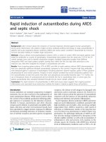
can be pipelined. Figure 3 shows the pipelined Loeffler’s fac-
torization with the lifting str u cture which is used in this pa-
per. Each addition, subtraction, and multiplication feeds a
delay in Figure 3. The symbol “D” denotes a delay for pur-
pose of pipelining.

3. IMPLEMENTATION OF THE CONSTANT
COEFFICIENT MULTIPLIERS
A constant-valued multiplication can be carried out by a se-
ries of additions and arithmetic shifts instead of using a mul-
tiplier [13]. For example, 15y is equivalent to 2
3
y +2
2
y +
2
1
y + y, where 2
n
is implemented as an arithmetic shift to
the left by n bits. Allowing subtr actions as well as additions
and arithmetic shifts reduces the number of required arith-
X
1
cos(α)
+
Y
1
sin(α)
−sin(α)
X
2
cos(α)
+
Y
2

(a)
X
1
++
Y
1
cos(α) − 1
sin(α)
sin(α)
cos(α) − 1
sin(α)
X
2
+ Y
2
(b)
Figure 2: Signal flow graph of (a) the plane rotation and (b) the
plane rotation with three lifting steps.
metic operations [13]. For example, 2
4
y − y is an alternate
implementation of 15y that requires one subtraction and
one arithmetic shift opposed to three additions and three
arithmetic shifts. Arithmetic shifts are essentially free in bit-
parallel implementations because they can be hardwired.
For convenience, the operations 2
3
y +2
2
y +2

1
y + y and
2
4
y − y can be expressed as signed binary numbers, 1111 and
1000 − 1, respectively. Each one or minus one digit is called a
nonzero element.
Acoefficient is said to be in canonic signed digit (CSD)
form when a minimum number of nonzero elements are
used to represent a coefficient value [13]. This results when
no two consecutive nonzero elements are present in the coef-
ficient. Examples of CSD coefficients are 1000 − 1, 1010101,
and 10 − 10001. CSD coefficients are preferred over binary
multiplications because of the reduced number of arithmetic
operations. Figure 4 shows the CSD implementation of a
constant coefficient multiplier of value 85.
3.1. Subexpression sharing
Subexpression sharing [14] can be used to further reduce the
coefficient complexity of CSD constant coefficient multipli-
ers. Numbers in the CSD format exhibit repeated subexpres-
sions of signed digits. For example, 101 is a subexpression
that occurs twice in 1010101. The coefficient complexity can
be reduced if the 101 subexpression is built only once and
is shared within the constant coefficient multiplier. In this
case, the coefficient complexity drops from three adders to
two adders. Figure 4 shows the implementation of a constant
coefficient multiplier of 85 using CSD coding and subexpres-
sion sharing. Subexpression sharing results in an implemen-
tation that can be up to fifty percent smaller than using CSD
coding [14]. All of the DCT implementations presented in

this paper use subexpression sharing.
546 EURASIP Journal on Applied Signal Processing
X
1
X
5
X
3
X
7
X
6
X
2
X
4
X
0
x
0
x
1
x
2
x
3
x
4
x
5

x
6
x
7
+++
8D
1/2
++
2D
−
+
6D
+
−
+ D
−
+
7D
p
1
u
1
+
−
+
3D
+
−
5D
−

+
3D
+
2D
+
2D
−
+
−
+3D
+
2D
−
+
3D
p
2
u
2
p
3
−
p
4
u
3
p
5
−
1/2

−
+
D
+
3D
+
−
+3D
−
+
D
−
+3D +
−
++ 2D
Figure 3: Signal flow graph of the pipelined Loeffler’s factor ization with the lifting structure.
x(n)
 2
 4
 6
+
+
+
y(n)
(a)
x(n)  2
+
 4
+
y(n)

(b)
Figure 4: Implementation of a constant coefficient multiplier of
value 85 using (a) CSD coding and (b) subexpression sharing.
4. PERFORMANCE MEASURES FOR FPGA-BASED DCT
APPROXIMATIONS
The DCT approximation-dependent and implementation-
dependent performance measures that can be controlled by
the method discussed in this paper include:
(1) coding gain;
(2) mean square error (MSE);
(3) hardware cost;
(4) quantization noise;
(5) power consumption.
Each performance m easure is defined below.
4.1. Coding gain
The coding gain (a measure of the degree of energy com-
paction offered by a transform [1]) is important in compres-
sion applications because it is proportional to the peak signal
to noise ratio (PSNR). Transforms with hig h coding gains
can be used to create faithful reproductions of the original
image with little error. The biorthogonal coding gain [15]is
defined as
C
g
= 10 log
10
σ
2
x



N−1
i=0
σ
2
x
i


f
i


2
2

1/N
, (4)
where  f
i

2
2
is the norm of the ith basis function, N is the
number of subbands (N = 8 for an eight-point DCT), σ
2
x
i
is
the variance of the ith subband, and σ

2
x
is the variance of the
input signal.
A zero mean unit variance AR(1) process with correlation
coefficient ρ = 0.95 is an accurate approximation of natural
images [10] and is used in our numerical experiments. The
variance of the ith subband is the ith diagonal element of R
yy
,
the autocorrelation matrix of the transformed signal
R
yy
= HR
xx
H
T
, (5)
where H is the forward transform matrix of the DCT trans-
form and R
xx
is the autocorrelation of the input signal. The
autocorrelation matrix R
xx
is symmetric and Toeplitz. The
elements in the first row, R
xx
1
, define the entire matrix
R

xx
1
=

1 ρ ··· ρ
N−1

. (6)
4.2. Mean square error
The MSE between the transformed data generated by the
exact and approximate DCTs quantifies the accuracy of the
DCT approximation. The MSE can be calculated determin-
istically [10] using the expression
MSE
=
1
N
Trace

DR
xx
D
T

, (7)
Rapid Prototyping of FPGA-Based DCT Approximations 547
In
X
X
2

−y
Q Out
(a)
In
X
X
2
−y
+
e
Out
(b)
Figure 5: Signal flow graph of (a) coefficient multiplier and (b) co-
efficient multiplier modeling quantization with the noise source e.
where D is the difference between the forward transform ma-
trix of the exact and approximate DCTs, and R
xx
is the auto-
correlation matrix of the input signal. It is advantageous to
have a low MSE value to ensure a near ideal DCT approxi-
mation.
4.3. Hardware cost
The hardware cost is the quantity of logic required to im-
plement a DCT approximation. On the Xilinx Virtex series
of FPGAs, the hardware cost is measured as the total num-
ber of slices required to implement the design. A Xilinx Vir-
tex slice contains two D-t ype flip-flops and two four-inputs
lookup tables. The Xilinx PAR process assigns logic functions
and interconnect to the slices, and can be used to gauge the
exact hardware cost. In recent years, the PAR runtimes have

dropped from hours to minutes for small to midrange de-
signs. Consequently, the PAR process can now be used di-
rectly by an optimization method to gauge the exact hard-
ware cost of a design. This paper presents a design method
for FPGA-based DCT approximations that uses the PAR to
provide the exact hardware cost of a design.
4.4. Quantization noise
A fixed-point constant coefficient multiplier can be imple-
mented as the cascade of an integer multiplier followed by a
power-of-two division (see Figure 5). Due to the limited pre-
cision of the datapath wordlength, it is not possible to repre-
sent the result of all divisions. Quantization becomes neces-
sary and occurs at the power-of-two division. A quantization
nonlinearity can be modeled as the summation of the signal
with a noise source [16] (see Figure 5).
If the binary point is in the right most position (all s ig-
nal values represent integers), then the maximum error in-
troduced in a multiplication is one for two’s complement
truncation arithmetic. A worst case bound, based on the L1
norm, on the quantization noise introduced by a coefficient
multiplication at the ith subband output [2], (
|N
a
i
|), is given
by


N
a

i


≤
L

k=1


g
ki


, (8)
In Q Out
(a)
In
+
e
Out
(b)
Figure 6: Signal flow graph of (a) the truncation of a datapath
wordlength and (b) the truncation of a datapath wordlength mod-
eling quantization with the noise source e.
where g
ki
is the feedforward gain from the output of the kth
multiplier to the ith subband output, and L is the number of
multipliers present in the transform.
Quantization through datapath wordlength truncation

can be arbitrarily introduced at any node (datapath) in a
DCT implementation to reduce hardware cost at the expense
of injected noise (see Figure 6)asdemonstratedin[3, 4]. A
worst case bound, based on the L1 norm, on the quantiza-
tion noise at the ith subband introduced through datapath
wordlength truncation, (|N
b
i
|), is given by


N
b
i


≤
P

k=1


h
ki



2
m
k

− 1

, (9)
where h
ki
is the feedforward gain from kth quantized node to
the ith subband output, m
k
is the number of bits truncated
from the LSB side of the wordlength at the kth node, and
P is the number of quantized datapath wordlengths present
in the transform. The total noise at the ith subband output
(|N
tot
i
|) is the sum of all scaled noise sources as given by


N
tot
i


=


N
a
i



+


N
b
i


. (10)
4.5. Power consumption
The power dissipated due to the switching activity in a
CMOS circuit [17] can be estimated using
P
= aC
tot
fV
2
, (11)
where a is the node transition factor, C
tot
is the total load
capacitance, f is the clock frequency, and V is the voltage of
the circuit. The node transition factor is the average number
of times a node makes a transition in one clock period.
The power consumption can be reduced by lowering the
clock frequency. Unfortunately a reduced clock rate lowers
the throughput and is not preferred for high-performance
compression systems that must process large amounts of
data. Lowering the supply voltage level reduces the power

consumption at the expense of a reduction in the maximum
clock frequency. Two alternatives remain. The load capaci-
tance and the node transition factor can be reduced. Subex-
pression sharing reduces both the node transition factor and
548 EURASIP Journal on Applied Signal Processing
the load capacitance of the constant coefficient multipliers.
The coefficient values and the datapath wordlengths can be
optimized to further reduce the node transition factor and
the total load capacitance of the DCT implementation.
The power consumption of the constant coefficient mul-
tipliers depends on the hardware cost and the logic depth
[18, 19, 20]. The hardware cost determines the total load ca-
pacitance. It is possible to reduce the power consumption by
lowering the hardware cost (using less slices and intercon-
nect). However, the hardware cost is a poor if not an incorrect
measure of the power consumption for constant coefficient
multipliers with a high logic depth as was observed in [18,
19, 20]. A transition in logic state must propagate through
more logic elements in a high-logic depth circuit, which in-
creases the power consumption. Transitions occur when the
signal changes value, and when spurious transitions, called
glitches, occur before a steady logic value is reached. High-
logic depth constant coefficient multipliers tend to use more
power than low-logic depth constant coefficient multipliers
irrespective of the hardware cost [18]. Subexpression sharing
produces low-cost and low-logic depth constant coefficient
multipliers [21], which reduces the amount of power.
It is possible to reduce the power consumption of the
constant coefficient multipliers by choosing coefficient val-
ues and datapath wordlengths that result in constant coeffi-

cient multiplier implementations with a reduced logic depth
and hardware cost [18].
4.5.1 Gauging the power consumption
The Xilinx ISE tool set includes a software package called
XPWR that can be used to estimate the power consump-
tion of a design implemented on a Xilinx Virtex FPGA. The
method discussed in this paper optimizes the coefficient val-
ues and the datapath wordlengths to yield a DCT implemen-
tation with the desired power consumption requirement.
XPWR is used to produce an estimate of the power consump-
tion whenever the design method requires a power consump-
tion figure.
5. PROBLEM STATEMENT AND FORMULATION
The design problem can be stated as follows: find a set of
coefficient values and datapath wordlengths, h, that yields
a DCT approximation with a high coding gain such that
the MSE, quantization noise, hardware cost, and power con-
sumption specifications are satisfied. This problem can be
formulated as a discrete constrained optimization problem:
minimize
−C
g
subject to
g
1
(h) = MSE(h) − MSE
max
≤ 0, (12)
g
2

(h) = SlicesRequired(h) − MaxSlices ≤ 0, (13)
g
3
(h) = EstimatedPower(h) − MaxPower ≤ 0, (14)
g
4
i
(h) =


N
tot
i


− MaxNoise
i
≤ 0fori = 0, ,7, (15)
where the constants MSE
max
, MaxPower, and MaxS-
lices are the largest permissible MSE, power consump-
tion, and hardware cost values, respectively. The functions
SlicesRequired(h) and EstimatedPower(h) yield the hardware
cost and the estimated power consumption, respectively. The
constant MaxNoise
i
is the largest permissible quantization
noise value in the ith subband. A one-dimensional DCT
approximation with eight subbands (which is used in the

JPEG and MPEG standards [1]) requires eight constraints
(i = 0, ,7) to control the quantization noise at each sub-
band output. Little if any quantization noise should contam-
inate the low-frequency subbands in compression applica-
tions because these subbands contain most of the signal en-
ergy. The high-frequency subbands can tolerate more quan-
tization noise since little signal energy is present in these sub-
bands. It is therefore advantageous to set differing quantiza-
tion noise constraints for each individual subband.
The above problem is difficult to solve analytically or nu-
merically because analytic derivatives of the objective func-
tion and constraints cannot be determined. Instead discrete
Lagrange multipliers can be used [22]. Fast discrete La-
grangian local searches have been developed [23, 24, 25] that
can be used to solve this discrete constrained optimization
problem. The constraints (12), (13), (14), and (15)canbe
combined to form a discrete Lagrangian function with the
introduction of a positive-valued scaling constant 
weight
and
the discrete Lagrange multipliers (λ
1
, λ
2
, λ
3
,andλ
4
i
)

L
d
=−
weight
C
g
+ λ
1
max

0,g
1
(h)

+ λ
2
max

0,g
2
(h)

+ λ
3
max

0,g
3
(h)


+
7

i=0
λ
4
i
max

0,g
4
i
(h)

.
(16)
6. A DISCRETE LAGRANGIAN LOCAL SEARCH
METHOD
The discrete Lagrangian local search was introduced in [22]
and later applied to filter bank design in [23] and peak con-
strained least squares (PCLS) FIR design in [24, 25]. The
discrete Lagrangian local search method presented here (see
Procedure 1) is adapted from the local search method pre-
sented in [24, 25].
6.1. Initialization of the algorithmic constants
The proposed method uses the following constants:
(i) λ
1
weight
, λ

2
weight
, λ
3
weight
, λ
4
weight
i
control the growth of the
discrete Lagrange multipliers;
(ii) 
weight
affects the convergence time of the local search
as discussed in [23];
(iii) MaxIteration is the largest number of iterations the al-
gorithm is permitted to execute.
Although experience shows hand tuning λ
1
weight
, λ
2
weight
,
λ
3
weight
, λ
4
weight

i
,and
weight
permits the design of DCT approxi-
mations with the highest coding gain given the constraints, it
is often time consuming and inconvenient. Instead, we in-
troduce an alternative initialization method. The algorith-
mic constants (
weight
, λ
1
weight
, λ
2
weight
, λ
3
weight
,andλ
4
weight
i
)can
be chosen to multiply the objective function and the con-
straints so that no constraint initially dominates the discrete
Lagrangian function, and the relative magnitude of (h)is
Rapid Prototyping of FPGA-Based DCT Approximations 549
Initialize the algorithmic parameters:
λ
1

weight
, λ
2
weight
, λ
3
weight
, λ
4
weight
i
,andMaxIteration
Initialize the discrete Lagrange multipliers:
λ
1
= 0, λ
2
= 0, λ
3
= 0, and λ
4
i
= 0fori = 0, ,7
Initialize the variables of optimization
h = Quantized DCT coefficients and full precision datapath wordlengths
While (not converged and not executed MaxIterations) do
change the current variable by ±1toobtainh

if L
d

(h

) <L
d
(h) then a ccept pr oposed change (h = h

)
update λ
1
once every three coefficient changes using
λ
1
← λ
1
+ λ
1
weight
max(0,g
1
(h))
update the following discrete Lagrange multipliers once every three iterations
λ
2
← λ
2
+ λ
2
weight
max(0,g
2

(h))
λ
3
← λ
3
+ λ
3
weight
max(0,g
3
(h))
λ
4
i
← λ
ij
4
+ λ
4
weight
i
max(0,g
4
i
(h)) for i = 0, ,7
end
Procedure 1: A local search method for the design of DCT approximations.
more easily weighted against the constraints. To this end, the
algorithmic constants can be initialized as follows:
λ

1
weight
=
1
MSE
max
, (17)
λ
2
weight
=
1
MaxSlices
, (18)
λ
3
weight
=
1
MaxPower
, (19)
λ
4
weight
i
=
1
MaxN oise
i
for i = 0, ,7, (20)


weight
=
θ

0
, (21)
where 
0
is the objective function evaluated using the quan-
tized DCT coefficients, and θ is a constant, 0 <θ<1, used
to control the quality of solutions and performance of the al-
gorithm. The local search favors DCT approximations with
high coding gain values when θ is close to one because the
objective function tends to dominate the discrete Lagrangian
function early in the search. However, the algorithm con-
verges at a slower rate because the discrete Lagrange multi-
pliers must assume a larger value, which requires more itera-
tions, before the constraints are satisfied. Small θ values per-
mit faster convergence at the expense of lower coding gain
values because the search favors minimizing the constraint
values over minimizing the objective function.
Equations (17), (18), (19), and (20) prevent any discrete
Lagrange multiplier from initially dominating the other dis-
crete Lagrange multipliers. The function g
2
(h) yields integer
values and g
4
i

(h) yields values greater than one that are of-
ten thousands of times larger than values produced by the
other constraints. Equally weighting λ
1
weight
, λ
2
weight
, λ
3
weight
,and
λ
4
weight
i
would bias the search to favor constraints (13)and
(15) over the remaining constraints.
6.2. Updating the coefficients and datapath
wordlengths
The variables of optimization, h, are composed of the coef-
ficient values and the datapath wordlengths. The coefficient
values are rational values (see Figure 5) of the form
coefficient =
x
2
CWL
, (22)
where x is an integer value that is determined during op-
timization and CWL is the coefficient wordlength which is

used to set the magnitude of the right shift.
The datapath wordlength is the number of bits used to
represent the signal in the datapath. The binary point posi-
tion of the input values to the DCT approximation can be ar-
bitrarily set [3]. The discussion in [3] places the binary point
to the left of the most sig nificant bit ( MSB) of the datapath
wordlength (all input values have a magnitude less than one).
In this paper, the binary point is placed in the right most po-
sition (all input values represent integers) which is consistent
with the literature on DCT-based compression [1].
The coefficients are initially set equal to the floating point
precision DCT coefficients rounded to the nearest permit-
ted finite precision value. The datapath wordlengths are set
wide enough to prevent overflow. The largest possible value
at the kth datapath wordlength in the DCT approximation is
bounded by


Max
k


≤
N−1

i=0


g
ik



M, (23)
where N is the number of DCT inputs, g
ik
is the feedforward
gain from the ith DCT input to the kth datapath, and M is the
largest possible input value (255 for the JPEG standard [1]).
The bit position of the MSB and the number of bits required
to fully represent the signal (excluding the sign bit) at the kth
550 EURASIP Journal on Applied Signal Processing
MSB
S
b
6
b
5
b
4
b
3
b
2
b
1
b
0
7bits
Binary point
MSB

Sb
6
b
5
b
4
b
3
b
2
b
1
0
6bits
Figure 7: A datapath wordlength of (a) seven bits and (b) the data-
path wordlength truncated to six bits.
datapath is
MSB
k
=

log
2

Max
k

. (24)
A datapath wordlength with more than MSB
k

bits is
wasteful and should not be used because the magnitude of
the maximum signal value can be represented using MSB
k
bits.
Each datapath wordlength and each coefficient value is
changed by ±1and±2
− CWL
, respectively, in a round robin
fashion, and each change is accepted if the discrete La-
grangian function decreases in value. Altering a coefficient
value changes the gains from the inputs to the internal nodes
that feed from the changed coefficient. Consequently, (23)
and (24) must be used to update the MSB positions for all of
the datapaths when a coefficient value is changed.
A reduction or increase in the datapath wordlength oc-
curs at the least significant bit (LSB) side of the datap-
ath wordlength. The binary point position (and hence the
value represented by the MSB) does not change despite any
changes in the datapath wordlength. The possibility of over-
flow is therefore excluded because the maximum value repre-
sented by the MSB of the datapath still exceeds the magnitude
of the largest possible signal value even though the datapath
precision may be reduced. Figure 7 shows a reduction from
seven bits to six bits in a datapath wordlength.
6.3. Updating the discrete Lagrange multipliers
If a constraint is not satisfied, then the respective discrete
Lagrange multiplier grows in value using the following re-
lations:
λ

1
←− λ
1
+ λ
1
weight
max

0,g
1
(h)

,
λ
2
←− λ
2
+ λ
2
weight
max

0,g
2
(h)

,
λ
3
←− λ

3
+ λ
3
weight
max

0,g
3
(h)

,
λ
4
i
←− λ
4
i
+ λ
4
weight
i
max

0,g
4
i
(h)

for i = 0, ,7.
(25)

The local search methods presented in [23, 24, 25] update
the discrete Lagrange multipliers once every three iterations
to prevent the random probing behavior discussed in [23].
However this u pdate schedule can produce poor results for
this optimization problem. The MSE is only a function of the
coeffi cients and not of the datapath wordlengths. The growth
of λ
1
depends only on the value of the coefficients. During
the optimization of the datapath wordlengths, λ
1
would con-
tinue to grow at a constant rate despite any changes in the
datapath wordlengths. The MSE begins to dominate the dis-
crete Lagrangian function resulting in higher objective func-
tion values. This problem is eliminated by updating λ
1
only
once every three changes in the coefficient values. The other
discrete Lagrange multipliers are updated once every three
iterations.
6.4. Local estimators of the hardware cost
and power consumption
A set of VHDL files that implement the DCT approximation
are produced before each PAR. Ideally, the design method
should perform a PAR every iteration. Although the r un
times for PARs have dropped dramatically, they still require
several minutes for designs presented in this paper. A typi-
cal runtime for the proposed method requires hours of com-
putation if a PAR is performed every iteration. To reduce

the runtime, it is possible to perform a PAR every N itera-
tions and estimate the hardware cost in between the PARs. A
hardware cost estimate, SlicesRequired(h), can be obtained
based on the number of full adders required by the cur-
rent DCT approximation, FullAdders(h), the number of full
adders required by the DCT approximation dur ing the last
PAR, FullAdders
PAR
, and the number of slices produced at
the last PAR, Slices
PAR
:
SlicesRequired(h) =
Slices
PAR
FullAdders
PAR
FullAdders(h). (26)
This provides a local estimate of the number of slices re-
quired to implement the DCT approximation.
In a similar fashion, a local estimate for the required
power, PowerEstimate(h), can be obtained based on the
power reported at the last PAR, Power
PAR
, and the previously
defined FullAdders
PAR
and FullAdders
PAR
:

PowerEstimate(h)
=
Power
PAR
FullAdders
PAR
FullAdders(h). (27)
The local search terminates when all of the constraints are
satisfied, the discrete Lagrangian function cannot be f urther
minimized, and when the local estimates of the hardware cost
and power consumption match the figures reported from the
Xilinx ISE toolset. These conditions ensure that the hard-
ware cost and power consumption figures at the discrete con-
strained local minimum are exact.
7. CONVERGENCE OF THE LOCAL SEARCH METHOD
The necessary condition for the convergence of a discrete La-
grangian local search occurs when all of the constr aints are
Rapid Prototyping of FPGA-Based DCT Approximations 551
satisfied, implying that h is a feasible solution to the design
problem. If any of the constraints is not satisfied, then the
discrete Lagrange multipliers of the unsatisfied constraints
will continue to grow in value to suppress the unsatisfied
constraints.
The discrete Lagrangian function equals the value of the
objective function when all of the constraints are satisfied.
The local search then minimizes the objective function. The
search terminates when all of the constraints are satisfied,
which prevents the growth of the discrete Lagrange multipli-
ers, and when h is a feasible local minimizer of the objective
function, which prevents changes to h. These conditions for

termination match the necessary and sufficient conditions
for the occurrence of a discrete constrained local minimum
[22]. Consequently, the search can only terminate w hen a
discrete constrained local minimum has b een located. (A for-
mal proof of this assertion is found in [22].) This property
holds for any positive nonzero values of λ
1
weight
, λ
2
weight
, λ
3
weight
,
and λ
4
weight
i
.
These constants control the speed of growth of the dis-
crete Lagrange multipliers and hence convergence time of
the search. More iterations are required to find a discrete
constrained local minimum if these constants assume a near
zero value, but experimentation suggests that lower objec-
tive function values can be expected and vise versa. Equations
(17), (18), (19), and (20)provideacompromisebetweenthe
convergence time and the quality of the solution.
The rate of convergence varies according to the design
specifications. Design problems with tight constraints re-

quire at most 1000 iterations to converge for designs consid-
ered in this paper. Design problems with no constraints on
the hardware cost or the power consumption require as little
as 50 iterations to converge.
7.1. Performance of the local search method
The use of the local estimators, (26)and(27), have been
found to decrease the runtime of the method discussed in
this paper by as much as a factor of twenty four. The speed
increase can be measured by comparing the runtimes of the
local search when using and not using the local estimators.
The following DCT approximation is used in this compar-
ison: MSE
max
= 1e-3, MaxNoise
j
= 48 for j = 0, ,7,
MaxSlices = 400, and MaxPower = 0.8W. Figure 8 shows
the hardware cost at each iteration using (26). The local
search requires 735 iterations and 16 PARs (N = 45) to con-
verge on a solution that satisfies all of the design constraints.
The local search requires 21 minutes of computation time to
solve this design problem on a Pentium II 400 MHz PC.
Large reductions in the hardware cost are obtained early
in the local search which leads to significant errors in the
hardware cost local estimator. These errors are corrected ev-
ery N iterations when the PAR is performed which causes the
large discontinuities seen at the beginning of Figure 8.The
accuracy of the local estimators improves as the hardware
cost approaches MaxSlices because smaller changes in the
DCT approximation are necessary to satisfy the constraints.

The local search terminates when all of the constraints are
satisfied, the discrete Lagrangian function cannot be f urther
minimized, and FullAdders
PAR
= FullAdders(h). The final
DCT approximation has a coding ga in of 8.8232 dB and the
MSE equals 1.6e-5.
The local search is now used to solve the same design
problem but a PAR is performed at every iteration. Figure 9
shows the hardware cost at each iteration. In this case, the lo-
cal search requires 882 iterations and 882 PARs to converge
on a solution that satisfies all of the design constraints. The
local search requires 503 minutes of computation time for
this design problem on a Pentium II 400 MHz PC. This run-
time is long and it may not be practical to explore the design
space.
The discrete Lagrangian function used in the second
numerical experiment differs from the discrete Lagrangian
function used in the first numerical experiment because the
local estimators are not used. Consequently, the local search
converges along a different path. The DCT approximation
obtained during this numerical experiment has a coding gain
of 8.8212 dB and the MSE equals 5.3e-5. More iterations are
required to converge in the second example but this is not al-
ways the case. The large discontinuities in Figure 8 do not ap-
pear in Figure 9 because the exact hardware cost is obtained
at each iteration.
8. CODING GAIN, MSE, AND HARDWARE COST
TRADE-OFF
Table 1 shows a family of FPGA-based DCT approximations.

Relaxing the constraint on the hardware cost (setting MaxS-
lices to a large number) produces a nearly ideal DCT approx-
imation. Entry 1 in Table 1 shows a near ideal DCT approx-
imation that produces low amounts of quantization noise at
the subband outputs since no data wordlength truncation
was necessar y to satisfy the hardware cost constraint.
The method presented in [2] was used to reduce the
quantization noise to only corrupt the LSB in the worst case
for all subbands except the DC subband. The input signal is
scaled above the worst case bound on the quantization noise
and the output is reduced by the same factor. A power-of-
two shift that exceeds the value of the worst case bound on
the quantization noise is an inexpensive factor for scaling be-
cause no additions or subtractions are required. The DC sub-
band does not suffer from any quantization noise since no
multipliers feed this subband.
The hardware cost for nearly eliminating the quantiza-
tion noise at each subband output is high and may not be
practical if only a limited amount of computational resources
are available to the DCT approximation. A trade-off between
the coding gain, MSE, and hardware cost is useful in design-
ing small DCT cores with high coding gain values that must
share limited space with other cores on an FPGA. The coding
gain varies as a direct result of varying the value of MaxSlices.
Entries 2 to 5 in Ta b le 1 show the trade-off between the
coding gain, MSE, and hardware cost for DCT approxima-
tions targeted for the XCV300-6 FPGA when the power con-
sumption is ignored, MSE
max
= 1e-3, MaxNoise

0
= 8,
552 EURASIP Journal on Applied Signal Processing
7016015014013012011011
Number of iterations
400
450
500
550
600
650
700
Hardware cost (slices)
Figure 8: The hardware cost during the design of a DCT approxi-
mation as measured using the local estimator (equation (26)).
MaxN oise
1
= 16, MaxNoise
j
= 32 for j = 2, ,6, and
MaxN oise
7
= 64. Entries 1 to 5 in Table 1 satisfy these con-
straints. This family of DCT approximations has small MSE
values and produces little quantization noise in the low fre-
quency subbands making it suitable for l ow cost compression
applications.
Entry 2 in Table 1 shows a near exact DCT approxima-
tion w i th a sig nificantly reduced hardware cost compared to
Entry 1. If the coding gain is critical, then this DCT approx-

imation is useful. By tolerating a slight reduction in the cod-
ing gain, the hardware cost can be reduced further. The D CT
approximation of Entry 5 in Tab l e 1 requires 208 less slices
(a reduction of thirty percent) than the DCT approximation
of Entry 2 in Ta b l e 1 and requires 438 less slices (a reduction
of forty-eight percent) than the DCT approximation of En-
try 1 in Ta ble 1. If coding gain is not critical, then this DCT
approximation may be appropriate. It is therefore possible
to use the proposed design method to find a suitable DCT
approximation for the hardware cost/performance require-
ments of the application.
Entry 6 in Ta b l e 1 shows the extreme of this trade-
off. This DCT approximation is very inexpensive at the ex-
pense of generating significantly more quantization noise
(the worst case bound on quantization noise in each subband
is 128). This DCT approximation may not be appropriate for
any application because of the severity of the quantization
noise.
851
801
751
701
651
601
551
501
451
401
351
301

251
201
151
101
51
1
Number of iterations
400
450
500
550
600
650
700
Hardware cost (slices)
Figure 9: The hardware cost during the design of a DCT approxi-
mation as measured using the PAR at each iteration.
9. CODING GAIN, MSE, AND POWER CONSUMPTION
TRADE-OFF
Atrade-off between the coding gain, the MSE, and the
power consumption is possible and useful in designing low-
power DCT approximations with high coding gain values.
Entries 2 to 4 of Table 2 show the trade-off between the cod-
ing gain and power consumption when MSE
max
= 1e-3,
MaxN oise
0
= 8, MaxNoise
1

= 16, MaxNoise
j
= 32 for
j = 2, ,6, and MaxNoise
7
= 64. The coding gain varies
as a direct result of varying MaxPower. Entry 1 in Tabl e 2
shows the power consumption of a near ideal DCT approx-
imation discussed in the previous section. Low-power DCT
approximations result from a slight decrease in coding gain
(compare entries 2 to 4 in Table 2). Entry 5 in Tabl e 2 shows
a low-power DCT approximation obtained at the expense of
significantly more quantization noise (the worst case bound
on quantization noise in each subband is 128).
10. CONCLUSION
A rapid prototyping methodology for the design of FPGA-
based DCT approximations (which can be used in lossless
compression applications) has been presented. This method
can be used to control the MSE, the coding gain, the level of
quantization noise at each subband output, the power con-
sumption, and the exact hardware cost. This is achieved by
Rapid Prototyping of FPGA-Based DCT Approximations 553
Table 1: Coding gain, MSE, hardware cost, and maximum clock frequency results for DCT approximations based on Loeffler’s factorization
using the lifting structure implemented on the XCV300-6 FPGA.
Entry number
Coding gain
MSE
Hardware cost Maximum clock
(dB) (slices) frequency (MHz)
1 8.8259 1.80e-8 912 117

2 8.8257 8.00e-6 682 129
3 8.8207 4.00e-5 600 135
4 8.7877 6.02e-4 530 142
5 8.7856 6.22e-4 474 135
6 7.8292 2.03e-2 313 142
Table 2: Coding gain, coefficient complexity, MSE, and power consumption results for DCT approximations based on Loeffler’s factorization
using the lifting structure implemented on the XCV300-6 FPGA with a clock rate of 100 MHz.
Entry number
Coding gain
MSE
Hardware cost Estimated power Measured power
(dB) (slices) consumption (W) consumption (W)
1 8.8259 1.80e-8 912 1.12 0.98
2 8.8257 8.00e-6 682 0.90 0.83
3 8.8201 2.70e-5 552 0.78 0.76
4 8.7856 6.22e-4 474 0.70 0.61
5 7.8292 2.03e-4 313 0.53 0.42
optimizing both the coefficient and datapath wordlength val-
ues which previously has not been investigated. Trade-offs
between the coding gain, the MSE, the hardware cost, and
the power consumption are possible and useful in finding a
DCT approximation suitable for the application.
ACKNOWLEDGMENT
This work was supported in part by the Natural Sciences and
Engineering Research Council of Canada.
REFERENCES
[1] K. Sayood, Introduction to Data Compression,MorganKauf-
mann Publishers, San Francisco, Calif, USA, 2000.
[2] T.W.FoxandL.E.Turner, “Lowcoefficient complexity ap-
proximations of the one dimensional discrete cosine trans-

form,” in Proc. IEEE Int. Symp. Circuits and Systems, vol. 1,
pp. 285–288, Scottsdale, Ariz, USA, May 2002.
[3] G. A. Constantinides, P. Y. K. Cheung, and W. Luk, “Heuristic
datapath allocation for multiple wordlength systems,” in Proc.
Design Automation and Test in Europe, pp. 791–796, Munich,
Germany, March 2001.
[4] W. Sung and K. I. Kum, “Simulation-based word-length opti-
mization method for fixed-point digital signal processing sys-
tems,” IEEE Trans. Signal Processing, vol. 43, no. 12, pp. 3087–
3090, 1995.
[5] A. Benedetti and P. Perona, “Bit-width optimization for con-
figurable DSP’s by multi-interval analysis,” in Proc.34thAsilo-
mar Conference on Signals, Systems and Computers, vol. 1, pp.
355–359, Pacific Grove, Calif, USA, November 2000.
[6] S. A. Wadekar and A. C. Parker, “Accuracy sensitive word-
length selection for algorithm optimization,” in International
Conference on Computer Design, pp. 54–61, Austin, Tex, USA,
October 1998.
[7] J.P.Heron,D.Trainor,andR.Woods, “Imagecompression
algorithms using re-configurable logic,” in Proc. 31st Asilomar
Conference on Signals, Systems and Computers, pp. 399–403,
Pacific Grove, Calif, USA, November 1997.
[8] N. W. Bergmann and Y. Y. Chung, “Efficient implementation
of DCT-based video compression on custom computers,” in
Proc. 31st Asilomar Conference on Signals, Systems and Com-
puters, pp. 1532–1536, Pacific Grove, Calif, USA, November
1997.
[9] C. Loeffler, A. Ligtenberg, and G. S. Moschytz, “Practical fast
1D DCT algorithms with 11 multiplications,” in Proc. IEEE
Int. Conf. Acoustics, Speech, Signal Processing, vol. 2, pp. 988–

991, Glasgow, Scotland, May 1989.
[10] J. Liang and T. D. Tran, “Fast multiplierless approximations
of the DCT with the lifting scheme,” IEEE Trans. Signal Pro-
cessing, vol. 49, pp. 3032–3044, December 2001.
[11] W. Sweldens, “The lifting scheme: A custom-design construc-
tion of biorthogonal wavelets,” Appl. Comput. Harmon. Anal.,
vol. 3, no. 2, pp. 186–200, 1996.
[12] I. Daubechies and W. Sweldens, “Factoring wavelet trans-
forms into lifting steps,” J. Fourier Anal. Appl.,vol.4,no.3,
pp. 247–269, 1998.
[13] R. I. Hartley and K. K. Parhi, Digit-Serial Computation,
Kluwer Academic Publishers, Boston, Mass, USA, 1995.
[14] R. I. Hartley, “Subexpression sharing in filters using canonic
signed digit multipliers,” IEEE Trans. on Circuits and Systems
II: Analog and Digital Sig nal Processing, vol. 43, no. 10, pp.
677–688, 1996.
[15] J. Katto and Y. Yasuda, “Performance evaluation of sub-
band coding and optimization of its filter coefficients,” in
Visual Communications and Image Processing, vol. 1605 of
SPIE Proceedings, pp. 95–106, Boston, Mass, USA, November
1991.
554 EURASIP Journal on Applied Signal Processing
[16] L. B. Jackson, “On the interaction of roundoff noise and dy-
namic range in digital filters,” Bell System Technical Journal,
vol. 49, no. 2, pp. 159–184, 1970.
[17] K. K. Parhi, VLSI Digital Signal Processing Systems ,JohnWiley
and Sons, New York, NY, USA, 1999.
[18] S. S. Demirsoy, A. G. Dempster, and I. Kale, “Transition anal-
ysis in multiplier-block based FIR filter structures,” in Proc.
IEEE International Conference on Electronic Circuits and Sys-

tems, pp. 862–865, Kaslik, Lebanon, December 2000.
[19] D. H. Horrocks and Y. Wongsuwan, “Reduced complexity
primitive operator FIR filters for low power dissipation,” in
Proc. European Conference Circuit Theory and Design, pp. 273–
276, Stresa, Italy, August 1999.
[20] D. Perello and J. Figueras, “RTL energy consumption metric
for carry-save adder trees: Application to the design of low
power digital FIR filters,” in Proc. 9th International Workshop
on Power and Timing Modeling, Optimization and Simulation,
pp. 301–311, Kos Island, Greece, October 1999.
[21] M. Martinez-Peiro, E. Boemo, and L. Wanhammar, “Design
of high speed multiplierless filters using a nonrecursive signed
common subexpression algorithm,” IEEE Trans. on Circuits
and Systems II: Analog and Digital Signal Processing, vol. 49,
no. 3, pp. 196–203, 2002.
[22] B. W. Wah and Z. Wu, “The theory of discrete Lagrange multi-
pliers for nonlinear discrete optimization,” in Proc. Principles
and Practice of Constraint Programming, pp. 28–42, Springer-
Verlag, Alexandria, Va, USA, October 1999.
[23] B.W. Wah, Y. Shang, and Z. Wu, “Discrete Lagrangian meth-
ods for optimizing the design of multiplierless QMF banks,”
IEEE Trans. on Circuits and Systems II: Analog and Digital Sig-
nal Processing, vol. 46, no. 9, pp. 1179–1191, 1999.
[24] T. W. Fox and L. E. Turner, “The design of peak constrained
least squares FIR filters with low complexity finite precision
coefficients,” in Proc. IEEE Int. Symp. Circuits and Systems,
vol. 2, pp. 605–608, Sydney, Australia, May 2001.
[25] T. W. Fox and L. E. Turner, “The design of peak constrained
least squares FIR filters with low complexity finite precision
coefficients,” IEEE Trans. on Circuits and Systems II: Analog

and Digital Signal Processing, vol. 49, no. 2, pp. 151–154, 2002.
Trevor W. Fox received the B.S. and Ph.D.
degrees in electrical engineering from the
University of Calgary in 1999 and 2002, re-
spectively. He is presently working for Intel-
ligent Engines in Calgary, Canada. His main
research interests include digital filter de-
sign, reconfigurable digital signal process-
ing, and rapid prototyping of digital sys-
tems.
Laurence E. Turner received the B.S. and
Ph.D. degrees in electrical engineering from
the University of Calgary in 1974 and 1979,
respectively. Since 1979, he has been a fac-
ulty member at the University of Calgary
where he currently is a Full Professor in
theDepartmentofElectricalandComputer
Engineering. His research interests include
digital filter design, finite precision effects
in digital filters and the development of
computer-aided design tools for digital system design.