Báo cáo hóa học: " A New Method for Estimating the Number of Harmonic Components in Noise with Application in High Resolution Radar" pdf

EURASIP Journal on Applied Signal Processing 2004:8, 1177–1188
c
 2004 Hindawi Publishing Corporation
A New Method for Estimating the Number
of Harmonic Components in Noise with
Application in High Resolution Radar
Emanuel Radoi
Laboratoire E3I2, Ecole Nationale Sup
´
erieure des Ing
´
enieurs des Etudes et Techniques d’Armement (ENSIETA),
2 rue Franc¸ois Verny, 29806 Brest, France
Email:
Andr
´
e Quinquis
Laboratoire E3I2, Ecole Nationale Sup
´
erieure des Ing
´
enieurs des Etudes et Techniques d’Armeme nt (ENSIETA),
2 rue Franc¸ois Verny, 29806 Brest, France
Email:
Received 18 Februar y 2003; Revised 8 December 2003; Recommended for Publication by Bjorn Ottersten
In order to operate properly, the superresolution methods based on orthogonal subspace decomposition, such as multiple signal
classification (MUSIC) or estimation of signal parameters by rotational invariance techniques (ESPRIT), need accurate estimation
of the signal subspace dimension, t hat is, of the number of harmonic components that are superimposed and corrupted by noise.
This estimation is particularly difficult when the S/N ratio is low and the statistical properties of the noise are unknown. Moreover,
in some applications such as radar imagery, it is very important to avoid underestimation of the number of harmonic components
which are associated to the target scattering centers. In this paper, we propose an effective method for the estimation of the signal

subspace dimension which is able to operate against colored noise with performances superior to those exhibited by the classical
information theoretic criteria of Akaike and Rissanen. The capabilities of the new method are demonstrated through computer
simulations and it is proved that compared to three other methods it carries out the best trade-off from four points of view, S/N
ratio in white noise, frequency band of colored noise, dynamic range of the harmonic component amplitudes, and computing
time.
Keywords and phrases: superresolution methods, subspace projection, discriminant function, high-resolution radar.
1. INTRODUCTION
There has been an increasing interest for many years in the
field of superresolution methods, such as multiple signal
classification (MUSIC) [1, 2] or estimation of signal par am-
eters by rotational invariance techniques (ESPRIT) [3, 4].
They have been conceived to overcome the limitations of the
Fourier-transform-based techniques, which are mainly re-
lated to the resolution achieved, especially when the num-
ber of available samples is reduced, and to the choice of the
weighting windows, which controls the sidelobe le vel. Fur-
thermore, there is always a tradeoff to do between the spatial
(spectral, temporal, or angular) resolution and the dynamic
resolution.
The most effective classes of superresolution methods di-
vide the observation space into two orthogonal subspaces
(the so-called signal subspace and noise subspace) and are
based on the autocorrelation matrix eigenanalysis. In con-
junction with signal subspace dimension estimation criteria,
they are well known to provide performances close to the
Cramer-Rao bound [5].
Akaike information criterion (AIC) [6] is one of the most
frequently used techniques to perform the estimation of the
signal subspace dimension in the case of the white Gaussian
noise. The number of harmonic components is determined

to achieve the best concordance between the model and the
observation data. Analytically, this condition is expressed in
the form
N = min
k

C(k)

,(1)
where C(k) is a cost function related to the log-likelihood
ratio of the model parameters for N
= k.
However, Rissanen demonstrated that the AIC yields an
inconsistent estimate and proposed the minimum descrip-
tion length (MDL) criterion [7] to overcome this prob-
lem. Although the estimate given by the MDL criterion is
1178 EURASIP Journal on Applied Signal Processing
consistent, the signal subspace dimension is underestimated,
especially when the number of samples is small.
In our experiments, we have used both the AIC and the
MDL criteria adapted by Wax and Kailath [8]. If P is the
number of independent realizations of length M, then the
cost functions in the two cases have the following expres-
sions,
AIC(k) =−2P(M − k)log


M
i=k+1
λ

1/( M−k)
i

1/(M − k)


M
i=k+1
λ
i

+2k(2M − k),
MDL(k) =−P(M − k)log


M
i=k+1
λ
1/( M−k)
i

1/(M − k)


M
i=k+1
λ
i

+

1
2
k(2M − k)logP,
(2)
where {λ
i
}
i=1, ,M
stand for the eigenvalues of the autocorre-
lation matrix.
When the noise statistics are unknown, other methods
have been proposed, such as the Gerschg
¨
orin disk technique
[9], known also as the Gerschg
¨
orin disk estimator (GDE) cri-
terion. It makes use of a set of disks, whose centers and radii
are both calculated from the autocorrelation matrix Σ.Let
A be the M × M matrix obtained by the following unitary
transformation,
A =





a
11
··· a

1M
.
.
.
.
.
.
.
.
.
a
M1
··· a
MM





= Q
H
ΣQ,(3)
where
Q =

q
1
··· q
M


,
q
k
=

1 e
j2πf
k
··· e
j2πf
k
(M−1)

T
√
M
, k = 1, , M,
(4)
are the orthogonal Fourier vectors so that q
k

2
= 1. The M
normalized frequencies are uniformly spaced from 0 to 1 −
1/M. It can be shown that a
kk
= q
H
k
Σq

k
∼
=
λ
k
. The centers of
the Gerschg
¨
orin disks are then given by C
k
= a
kk
, while their
radii by R
k
=

M
i=1, i=k
|a
ki
|. The cost function is expressed in
the form
GDE(k) = dist(k) −
δ
M
M

i=1
dist(i), (5)

where
dist(k)
=





C
k
C
max

2
+

R
k
R
max

2
(6)
are sorted in decreasing order. The choice of the coefficient δ
is somehow arbitrary. Its value should be dependent only on
the autocorrelation matrix dimension M according to [10],
where it is set to 1. However, we found out that it also de-
pends on the number of harmonic components to be esti-
mated. Although this dependence is weak, it results in signif-
icant differences in terms of detection performance when a

random number of sinusoids are superimposed with respect
to the case when the signal contains only two harmonic com-
ponents, as it is shown in Section 4.
The solution is considered to be the argument which
yields the last positive value of the cost function defined
above. Although GDE method performs b etter than AIC and
MDL for colored noise, it is less effective for white noise and
significantly increases the computing time compared to these
two criteria.
The method we propose in this paper for the estimation
of the signal subspace dimension performs the best tradeoff
in terms of robustness to white noise, robustness to colored
noise, dynamic range of the spectral components, and com-
puting time.
The rest of the paper is organized as follows. The princi-
ple of the new criterion and the associated cost function are
described in Section 2. Section 3 gives an analytical demon-
stration for a simplified, but representative, variation of the
autocorrelation matrix eigenvalues. Section 4 provides some
convincing results which prove the capabilities of the pro-
posed method and validate it on the example of a radar range
profile reconstruction using the MUSIC technique. General
conclusion is drawn in Section 5 together with some perspec-
tives about our future research work.
2. NEW CRITERION DERIVATION
The variation of the autocorrelation matrix eigenvalues is di-
rectly related to the number of harmonic components ( N)
present in the analyzed signal. Indeed, there are exactly N
nonzero eigenvalues in the noiseless case, while if an addi-
tive white Gaussian noise (AWGN) is considered, the M

− N
smallest eigenvalues should all equal to the noise variance
[11].
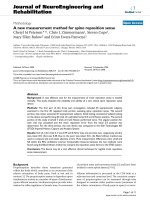
An example is provided on Figure 1 for the case of the
superposition of 2 sinusoids (N = 4) corrupted by AWGN.
Thus, for large S/N ratios the number of significant eigenval-
ues equals the number of harmonic components, the others
taking values close to zero, as it can be seen on Figure 1a.
When the noise level increases, the N largest eigenvalues are
still associated to the eigenvectors which span the signal sub-
space,butitismuchmoredifficult to make a robust deci-
sion using only their simple variation. Thus, the dist ribu-
tion of the eigenvalues associated to the noise subspace is not
uniform, as predicted in theory, because of the small num-
ber of data samples considered, while the transition between
the two classes of eigenvalues becomes less and less marked
(Figure 1b).
Consequently, the distribution of the autocorrelation
matrix eigenvalues cannot be considered a reliable criterion
for estimating the number of harmonic components, when
the S/N ratio is weak, no matter whether the noise is white
or not. However, the AIC and MDL criteria demonstrate
that even if a simple thresholding is not able to provide this
Estimation of Number of Components for High Resolution Algorithms 1179
0 1 2 3 4 5 6 7 8 9 10 11
k
0
0.5
1
1.5

2
2.5
3
3.5
4
Autocorrelation matrix eigenvalues
(a)
01234567891011
k
0
1
2
3
4
5
6
7
Autocorrelation matrix eigenvalues
(b)
Figure 1: Variation of the autocorrelation matrix eigenvalues for 2 superimposed sinusoids corrupted by white Gaussian noise, (a) S/N =
30 dB and (b) S/N = 5dB.
Signal subspace
Noise subspace
012345678910
k
0
0.05
0.1
0.15
0.2

0.25
0.3
0.35
Discriminant functions
(a)
012345678910
k
−0.2
−0.1
0
0.1
0.2
0.3
Cost function
(b)
Figure 2: Ideal shapes of (a) the discriminant functions and (b) the associated cost function, for N = 4.
estimate, the eigenvalue variation can be still used, in a dif-
ferent form, for obtaining N.
The main idea behind the new method is that estimat-
ing N is equivalent to finding how many eigenvalues are
associated to each of the two subspaces, signal and noise. This
can be considered a classification problem with two classes,
whose separation limit can be found using two discriminant
functions to be defined. In the ideal case, for the example
given above, these functions should have the shapes shown
on Figure 2a. They have been normalized so that they can be
considered equivalent probability density functions (pdf) as-
sociated to the two classes.
This approach, which makes use of discriminant func-
tions instead of the probabilities, is considered to be an effec-

tive alternative to the Bayes decision approach in the pattern
classification theory. While suboptimality may still occur be-
cause of improper choice of the discriminant functions, as
in the case of incorrect distribution assumption in the Bayes
approach, the discriminant function based method usually
offers implementational simplicity and it may be possible to
circumvent the data consistency issue [12].
If g
1
and g
2
denote the two discriminant functions, then a
new cost function, represented on Figure 2b,canbedefined
in the form
C
new
(k) = g
1
(k) − g
2
(k). (7)
1180 EURASIP Journal on Applied Signal Processing
Signal subspace
Noise subspace
012345678910
k
−0.05
0
0.05
0.1

0.15
0.2
0.25
0.3
0.35
0.4
0.45
Discriminant functions
(a)
0 1 2 3 4 5 6 7 8 9 10 11
k
−0.2
−0.1
0
0.1
0.2
0.3
0.4
Cost function
(b)
Figure 3: Real shapes of (a) the discriminant functions and (b) the associated cost function, for N = 4andS/N = 5dB.
Just like in the case of the GDE criterion, the solution N is
obtained as the argument which yields the last positive value
of this cost function.
We will present in the following the proposed forms for
the two discriminant functions g
1
and g
2
.Theyhavebeende-

duced in an empirical way, using some remarks on the behav-
ior of the autocorrelation matrix eigenvalues (see Section 3).
The values {λ
k
}
k=1, ,M
can be considered as their mem-
bership measures with respect to the signal subspace. Conse-
quently, in order to approximate the first ideal shape shown
on Figure 2a, the function g
1
is chosen as the variation of the
last M − 1 eigenvalues sorted in decreasing order and nor-
malized in order to obtain an equivalent probability density
function
g
1
(k) =
λ
k+1

M
i=2
λ
i
, k = 1, , M − 1. (8)
The variation of the second discriminant function should
capture in a suitable way the jump from the last eigenvalue
associated to the signal subspace and the first eigenvalue as-
sociated to the noise subspace. As it was stated above, it is dif-

ficult to detect directly this jump in the case of noisy signals.
However, it can be noticed that even for these signals there is
a slope variation between the two classes of eigenvalues. The
main idea for defining the second discriminant function is
then to exploit this slope variation to distinguish between the
two classes. Thus, the function g
2
, corresponding to the noise
subspace, is chosen to have an inverse variation with respect
to the function g
1
andisdefinedasanequivalentprobability
density function too,
g
2
(k) =
ξ
k

M−1
i=1
ξ
i
, k = 1, , M − 1, (9)
where ξ
k
= 1 −α(λ
k
−µ
k

)/µ
k
and µ
k
= (1/(M − k))

M
i
=k+1
λ
i
and α is taken so that α max
k
[(λ
k
− µ
k
)/µ
k
] = 1.
Note that {ξ
k
}
k=1, ,M
mainly measures the relative slope
variation of the eigenvalues {λ
k
}
k=1, ,M
.Thedifference be-

tween the current eigenvalue and the mean of the next ones
has been preferred to the simple subtraction of the next
eigenvalue in order to integrate the irregular eigenvalue vari-
ation. A smoother form of the second discriminant function
can be thus obtained.
The shapes of the two discriminant functions calculated
with (8)and(9), for the example given above, are represented
on Figure 3a. The corresponding cost function is also repre-
sented on Figure 3b. Note that even if the real shapes of the
discriminant functions approximate rather poorly the ideal
ones, the cost function issued from their difference allows
quite satisfactorily the estimation of N.
3. PARTICULAR CASE OF A LINEAR PIECEWISE
VARIATION OF THE AUTOCORRELATION
MATRIX EIGENVALUES
The theoretical validity of this criterion will be demonstrated
in the following, on the simplified case of the linear variation
of the autocorrelation matrix eigenvalues, as illustrated on
Figure 4. It can be expressed in the following form,
λ
k
=



b − ak, k = 1, , N,
d − ck, k = N +1, , M.
(10)
There are some important elements concerning this fig-
ure to be discussed. When the noise is white, the smallest

M − N eigenvalues should be all equal to the noise vari-
ance. In practice it is never true, because the noise is never
Estimation of Number of Components for High Resolution Algorithms 1181
MN +1N210
k
∆λ
2
d − ck
∆λ
1
b −ak
λ
k
Figure 4: Piecewise linear model for the variation of the autocorre-
lation matrix eigenvalues.
completely white. The more colored is the noise, the larger is
the dynamic range ∆λ
2
.
The N largest eigenvalues are related to the harmonic sig-
nal component. The value of ∆λ
1
is mainly given by the fre-
quency gap between the closest components. The closer they
are, the larger is the dynamic range ∆λ
1
.
The eigenvalue variation is not necessarily linear, but the
results obtained in this case can be generalized. This type of
variation has also the advantage of being the simplest model

which is able to integrate the elements related to the most
difficult components to be resolved and to the noise charac-
teristics.
The slopes corresponding to the eigenvalue variation in
the two domains represented on Figure 4 can be readily cal-
culated,
∆λ
1
= a(N − 1) =⇒ a =
∆λ
1
N − 1
,
∆λ
2
= c(M − N − 1) =⇒ c =
∆λ
2
M − N −1
.
(11)
The eigenvalues are usually normalized so that
λ(1)
= 1 =⇒ b = a +1=⇒ b = 1+
∆λ
1
N − 1
. (12)
Because even the smallest eigenvalue must be positive,
the follow ing condition has to be met,

d − cM > 0 =⇒ d = ε +
M
M − N −1
∆λ
2
, (13)
with ε>0, but ε  1.
Obviously, it is necessary to insure that the smallest
eigenvalue corresponding to the signal subspace is larger than
the largest eigenvalue corresponding to the noise subspace,
λ(N) >λ(N +1)
=⇒ 1 − ∆λ
1
>ε+ ∆λ
2
. (14)
The eigenvalue variation can be rewritten now in the fol-
lowing form,
λ(k) =









1 −
∆λ

1
N − 1
(k − 1), k = 1, , N,
ε +
∆λ
2
M − N −1
(M − k), k = N +1, , M.
(15)
In order to build the first discriminant function as a pdf,
the fol lowing sum is calculated,
S
1
=
M

k=2
λ(k)
= N − 1 −
N
2
∆λ
1
+
(M − N)(M + N −1)
2(M − N −1)
∆λ
2
+(M − N)ε.
(16)

The function g
1
(k) can be therefore expressed as
g
1
(k) =
1
S
1
λ(k +1)
=











1
S
1

1 −
∆λ
1
N − 1

k

, k = 1, , N − 1,
1
S
1

ε +
∆λ
2
M − N −1
(M − k)

, k = N, , M − 1.
(17)
The first step for calculating the second discriminant
function g
2
(k) consists in expressing the partial eigenvalue
average
µ(k) =
1
M − k
M

j=k+1
λ( j)
=






















1
M − k

S
1
+1− k −
∆λ
1
N − 1
k(k − 1)
2


,
k = 1, , N,
ε +
∆λ
2
2(M − N −1)
(M − k +1),
k = N +1, , M − 1.
(18)
The expression of µ(k)from1toN has been obtained by
taking into account that

M
j=k+1
λ( j) = S
1
−

k
j=2
λ( j). The
previous result leads to
η(k) =
λ(k) − µ(k)
µ(k)
=






















2(N − 1)

M − S
1
− 1

− ∆λ
1
(k − 1)(2M − 3k)
2(N − 1)

S

1
+1− k

− ∆λ
1
k(k − 1)
,
k
= 1, , N,

(M − k +1)/2(M − N +1)

∆λ
2
ε +

(M − k +1)/2(M − N +1)

∆λ
2
,
k = N +1, , M − 1.
(19)
Note that even for the simplest case of a linear model for
the eigenvalue variation, it becomes too complicated to con-
tinue using the exact forms of the expressions deduced above.
That is why the following approximations will be considered
hereinafter,
∆λ
2

 1, ∆λ
2
 ∆λ
1
, ε  1. (20)
1182 EURASIP Journal on Applied Signal Processing
Amuchsimplerformforη(k) is obtained, taking into
account these approximations,
η(k)
∼
=

















M − N
N − k

, k = 1, , N − 1,
2

1 − ∆λ
1

2ε + ∆λ
2
, k = N,
1, k = N +1, , M − 1.
(21)
Themaximumvalueofthisfunctionisobtainedfork
=
N. It can be consequently normalized and then transformed
into the second discriminant function,
h(k) = 1 − η
norm
(k)
∼
=














1 −
1
η(N)
M − N
N − k
, k = 1, , N − 1,
0, k = N,
1 −
1
η(N)
, k = N +1, , M − 1.
(22)
The final form of the second discriminant function is ob-
tained by simply t ransforming the function h(k) into a pdf,
which means to normalize it to the following sum,
S
2
=
M−1

k=1
h(k)
∼
=
M − (M − N − 1)
2ε + ∆λ
2

2

1 − ∆λ
1

.
(23)
Consequently, the following form is finally obtained for
the second discriminant function,
g
2
(k) =
h(k)
S
2
=
















1
S
2

1 −
1
η(N)
M − N
N − k

, k = 1, , N − 1,
0, k = N,
1
S
2

1 −
1
η(N)

, k = N +1, , M − 1.
(24)
Using the same approximations as indicated above, the
first discriminant function becomes
g
1
(k)
=












1 −

∆λ
1
/(N − 1)

k
N

1 − ∆λ
1
/2

− 1
, k = 1, , N − 1,
(M − k)∆λ
2
(M − N −1)

N


1 − ∆λ
1
/2

− 1

, k = N, , M − 1.
(25)
The values of the two discriminant functions corre-
sponding to the arguments N and N + 1 are to be calculated
in order to demonstrate that the solution of the problem
is N,
g
1
(N) =
∆λ
2

(M − N)/(M − N − 1)

N

1 − ∆λ
1
/2

− 1
,
g

1
(N +1)=
(1 + ε)∆λ
2
N

1 − ∆λ
1
/2

− 1
,
g
2
(N) = 0,
g
2
(N +1)
=
2

1 − ∆λ
1

− 2ε − ∆λ
2
2(N −1)

1−∆λ
1


+(M−N −1)

2

1−∆λ
1

−2ε−∆λ
2

∼
=
1
M
.
(26)
It is obvious from these relationships that
g
1
(N) >g
2
(N). (27)
On the other hand,
g
1
(N +1)<g
2
(N +1)⇐⇒ (1 + ε)∆λ
2

<
N − 1 − (N/2)∆λ
1
M
.
(28)
If the limit value for ∆λ
1
is considered, that is, ∆λ
1
= 1,
the fol lowing inequality is obtained,
(1 + ε)∆λ
2
<
N/2
− 1
M
. (29)
This means that in the worst case the solution of the
problem is still N if the noise power and whiteness are so
that the condition above is accomplished. It corresponds to
S/N ratios lower than those from the validity domain of the
Akaike and Rissanen criteria.
4. SIMULATION RESULTS
Three types of computer simulations have been conducted in
order to demonstrate the capabilities of the new method.
A superposition of two sinusoids (N = 4), corrupted by
an additive white Gaussian noise, has been firstly considered.
Since the number of samples is 16, two harmonic compo-

nents cannot be resolved by Fourier analysis if their normal-
ized frequencies are closer than 1/16 = 0.0625. For each S/N
ratio between 0 and 20 dB, 10000 independent simulations
have been performed for calculating the detection rate. The
two normalized frequencies associated to the two sinusoids
are chosen randomly for each iteration so that the distance
between them is between 1/32 and 1/16.Theresultsarepre-
sented on Figure 5.
Note that the proposed criterion slightly outperforms the
AIC and MDL criteria in terms of detection rate (Figure 5a).
Figures 5b and 5c illustrate the mean estimate and vari-
ance variations. They indicate a very interesting behavior of
the new method. Thus, it can be readily seen (Figure 5b)
that it is the only among the four criteria that overestimates
Estimation of Number of Components for High Resolution Algorithms 1183
AIC criterion
MDL criterion
GDE criterion
New criterion
0 5 10 15 20
S/N ratio (dB)
0
0.1
0.2
0.3
0.4
0.5
0.6
0.7
0.8

0.9
1
Detection rate
(a)
AIC criterion
MDL criterion
GDE criterion
New criterion
0 5 10 15 20
S/N ratio (dB)
1
1.5
2
2.5
3
3.5
4
4.5
5
5.5
Average
(b)
AIC criterion
MDL criterion
GDE criterion
New criterion
0 5 10 15 20
S/N ratio (dB)
−40
−35

−30
−25
−20
−15
−10
−5
0
5
Var iance
(c)
AIC criterion
MDL criterion
GDE criterion
New criterion
0 5 10 15 20
S/N ratio (dB)
0
0.1
0.2
0.3
0.4
0.5
0.6
0.7
0.8
0.9
1
Detection rate
(d)
Figure 5: Performance of the four criteria for the case of two superimposed sinusoids with the same magnitude: (a) detection rate against

white noise, (b) estimate mean, (c) estimate variance, and (d) detection rate against colored noise (a = 0.75).
the number of harmonic components for low S/N ratios.
This is particularly important in superresolution radar im-
agery applications, where underestimation has to be always
avoided because it leads to lost scattering centers in the
reconstructed image of the radar target. It is also obvi-
ous that the new criterion is the most consistent because
its variance, expressed in dB on Figure 5c, decreases the
fastest.
The variation of the detection rate corresponding to the
four criteria for a colored noise is presented on Figure 5d.
The colored noise has been obtained by filtering the white
noise using an AR filter of order 1, defined by its denomi-
nator coefficient a, which has been chosen as 0.7 for the ex-
ample g iven here. Note that the new criterion clearly out-
performs again both the AIC and MDL cr iteria, being in the
same time less robust than the GDE criterion.
1184 EURASIP Journal on Applied Signal Processing
AIC criterion
MDL criterion
GDE criterion
New criterion
0246810
Dynamic range (dB)
0
0.1
0.2
0.3
0.4
0.5

0.6
0.7
0.8
0.9
1
Detection rate
(a)
AIC criterion
MDL criterion
GDE criterion
New criterion
00.10.20.30.40.50.60.70.80.9
AR filter coefficient
0
0.1
0.2
0.3
0.4
0.5
0.6
0.7
0.8
0.9
1
Detection rate
(b)
Figure 6: Performance of the four criteria for the case of two superimposed sinusoids: ( a) detection rate against white noise (S/N = 10 dB)
and different magnitudes of the harmonic components and (b) detection rate against colored noise (S/N = 15 dB) and the same magnitude
of the harmonic components.
0.8

0.6
0.4
0.2
0
First pole
0.5
0
Second pole
0
0.5
1
Detection rate
(a)
0.8
0.6
0.4
0.2
0
First pole
0.5
0
Second pole
0
0.5
1
Detection rate
(b)
0.8
0.6
0.4

0.2
0
First pole
0.5
0
Second pole
0
0.5
1
Detection rate
(c)
0.8
0.6
0.4
0.2
0
First pole
0.5
0
Second pole
0
0.5
1
Detection rate
(d)
Figure 7: Performance of the four criteria for the case of two superimposed sinusoids with the same magnitude corrupted by a second-order
AR random process (S/N = 15 dB): (a) AIC criterion, (b) MDL cr iterion, (c) GDE criterion, and (d) new criterion.
Estimation of Number of Components for High Resolution Algorithms 1185
AIC criterion
MDL criterion

GDE criterion
New criterion
0 5 10 15 20 25 30
S/N ratio (dB)
0
0.1
0.2
0.3
0.4
0.5
0.6
0.7
0.8
0.9
1
Detection rate
(a)
AIC criterion
MDL criterion
GDE criterion
New criterion
0 5 10 15 20 25 30
S/N ratio (dB)
0
0.1
0.2
0.3
0.4
0.5
0.6

0.7
0.8
0.9
1
Detection rate
(b)
AIC criterion
MDL criterion
GDE criterion
New criterion
0 5 10 15 20 25 30
S/N ratio (dB)
0
0.1
0.2
0.3
0.4
0.5
0.6
0.7
0.8
0.9
1
Detection rate
(c)
AIC criterion
MDL criterion
GDE criterion
New criterion
0 5 10 15 20 25 30

S/N ratio (dB)
0
0.1
0.2
0.3
0.4
0.5
0.6
0.7
0.8
0.9
1
Detection rate
(d)
Figure 8: Performance of the four criteria for the case of a random number of superimposed sinusoids uniformly frequency spaced and
having the same mag nitude: (a) detection rate against white noise, (b) detection rate against colored noise (a = 0.75), (c) detection rate
against colored noise (a = 0.9), and (d) detection rate against colored noise (a = 0.95).
A more complete study has been performed on the be-
havior of the four criteria, with respect to the dynamic range
of the amplitudes of the two sinusoids (Figure 6a) and to the
whiteness of the noise (Figure 6b). S/N ratios of 10 dB and
15 dB, respectively, have been considered in the two cases. As
it can be seen, the AIC and MDL criteria perform better when
the dynamic range of the amplitudes is larger than 3 dB, but
they are much less robust than the other two criteria for col-
ored noise.
We have also evaluated the performance of the four com-
pared criteria when the signal is corrupted by a second-order
AR random process (Figure 7). The two poles of the white-
noise-driven AR filter take values between 0 and 0.95, with

an increment of 0.05.
1186 EURASIP Journal on Applied Signal Processing
Ideal
MUSIC
0 5 10 15 20 25
x[m]
0
0.2
0.4
0.6
0.8
1
1.2
1.4
A
(a)
1234567
k
−0.1
−0.05
0
0.05
0.1
0.15
0.2
0.25
0.3
0.35
New criterion function
(b)

Ideal
MUSIC
0 5 10 15 20 25
x[m]
0
0.2
0.4
0.6
0.8
1
1.2
1.4
A
(c)
1234567
k
−0.1
−0.05
0
0.05
0.1
0.15
0.2
0.25
0.3
0.35
New criterion function
(d)
Figure 9: Estimation of the number of the scattering centers of a radar target by the proposed method: (a) peak estimation using MUSIC
technique, (b) cost function variation for S/N = 25 dB, (c) peak estimation using MUSIC technique, and (d) cost function variation for

S/N = 10 dB.
Just like in the case of the first-order AR random process,
the detection rate obtained using the new approach begins
to decrease when the two poles start approaching simulta-
neously the unit circle so that the proposed method is ob-
viously outperformed by the GDE c riterion in its neigh bor-
hood. However, it performs better than the AIC and MDL
criteria for a wide range of variation of the two poles.
A random number of harmonic components has been
considered in the second phase of computer simulations. In
this case, al l the superimposed sinusoids have the same mag-
nitude and are uniformly frequency spaced, the normalized
frequencies of two successive components being separated by
0.06. The results are given on Figure 8, for four values of the
AR filter coefficient, 0, 0.75, 0.9, and 0.95.
The S/N ratio domain has been extended because the
GDE criterion reaches the maximum value of the detection
rate around 30 dB, compared to 20 dB for the case of two si-
nusoids. Hence, it is clear that the detection performance of
this method depends on the number of harmonic compo-
nents to be detected, as we have already stated in Section 1.
It is also important to note that the new criterion performs
again better than the AIC and MDL criteria for all the S/N
ratios and even better than the GDE criterion if the AR coef-
ficient is up to 0.9.
Finally, the third type of simulations have been devoted
to a high-resolution r adar application. The goal is to fi nd the
most accurate estimate of the range profile of a radar tar-
get using its complex signature in the frequency domain. An
Estimation of Number of Components for High Resolution Algorithms 1187

AIC & MDL
GDE
New criterion
0 50 100 150 200 250 300
Number of samples
0
5
10
15
20
25
30
35
Computing time
Figure 10: Computing time required by the four criteria over 10000
independent simulations and different numbers of samples.
illustrative example is shown on Figure 9 for the case of five
scattering centers. Their positions along the line of sight are
recovered very precisely using the MUSIC technique, while
their number is correctly estimated by the new criterion de-
fined above. Note that even for low S/N ratios, the associ-
ated cost function gives an appropriate and unambiguous
result.
The last comparison of the four criteria has been per-
formed with respect to the computing time required to esti-
mate the number of harmonic components. It has been mea-
sured over 10000 independent simulations and for different
numbers of samples from 16 to 256. The results which are
given on Figure 10 have been obtained on a PC Pentium IV,
operating at 650 MHz.

5. CONCLUSION
A new method is proposed in the paper for estimating the
number of harmonic components in colored noise. Its prin-
ciple is based on the original idea which consists in refor-
mulating the estimation problem as a classification problem
with two classes. An analytical demonstration is provided for
a special case of a piecewise linear variation of the autocorre-
lation matrix eigenvalues. Although this model is very sim-
ple, it contains all the essential information related to the
number of the harmonic components, to the power and the
whiteness of the noise, and to the closest spectral compo-
nents.
The new method has been compared to AIC, MDL, and
GDE techniques and its capabilities have been evaluated from
the point of view of the supported dynamic range of the har-
monic component magnitudes, of its behavior against white
and colored noise, and of the required computing time. We
found out that the new criterion realizes the best tradeoff in
estimating the signal subspace dimension. Thus, it performs
better than AIC and MDL methods, in white and especially
colored noise, and it has a better behavior than the GDE cri-
terion against white noise and with respect to the amplitude
dynamic range. It is still better than this one, even against col-
ored noise, for a wide range of the associated frequency band.
It is also the fastest among the criteria mentioned above. Fi-
nally, it is the only method which overestimates the number
of harmonic components, for low S/N ratios and small num-
ber of samples.
This last property makes our method particularly useful
in radar imagery applications, where it is preferable to over-

estimate the number of scattering centers than underestimate
it. Hence, as future work, we plan to use it in the context of
our ongoing research concerning the robust reconstruction
and classification of radar target images by superresolution
methods [13, 14].
REFERENCES
[1] G. Bienvenu and L. Kopp, “Adaptivity to background noise
spatial coherence for high resolution passive methods,” in
Proc. IEEE Int. Conf. Acoustics, Speech, Signal Processing,pp.
307–310, Denver, Colo, USA, April 1980.
[2] R. O. Schmidt, A signal subspace approach to multiple emitter
location and spectral estimation, Ph.D. thesis, Stanford Uni-
versity, Stanford, Calif, USA, 1981.
[3] A. Paulraj, R. Roy, and T. Kailath, “A subspace rotation ap-
proach to signal parameter estimation,” Proc. IEEE, vol. 74,
no. 7, pp. 1044–1045, 1986.
[4] R. Roy and T. Kailath, “ESPRIT—Estimation of signal param-
eters via rotational invariance techniques,” IEEE Trans. Acous-
tics, Speech, and Signal Processing, vol. 37, no. 7, pp. 984–995,
1989.
[5] P. Stoica and T. S
¨
oderstr
¨
om, “Statistical analysis of MUSIC
and subspace rotation estimates of sinusoidal frequencies,”
IEEE Trans. Signal Processing, vol. 39, no. 8, pp. 1836–1847,
1991.
[6] H. Akaike, “A new look at the statistical model identification,”
IEEE Trans. Automatic Control, vol. AC-19, no. 6, pp. 716–723,

1974.
[7] J. Rissanen, “Modeling by shortest data description,” Auto-
matica, vol. 14, no. 5, pp. 465–471, 1978.
[8] M. Wax and T. Kailath, “Detection of signals by information
theoretic criteria,” IEEE Trans. Acoustics, Speech, and Signal
Processing, vol. 33, no. 2, pp. 387–392, 1985.
[9] H T. Wu, J F. Yang, and F K. Chen, “Source number estima-
tors using transformed Gerschgorin radii,” IEEE Trans. Signal
Processing, vol. 43, no. 6, pp. 1325–1333, 1995.
[10] O. Caspary and P. Nus, “New criteria based on Gerschgorin
radii for source number estimation,” in Proc. European Sig-
nal Processing Conference, vol. I, pp. 77–80, Rhodes, Greece,
September 1998.
[11] L. Marple, DigitalSpectralAnalysiswithApplications,
Prentice-Hall, Englewood Cliffs, NJ, USA, 1987.
[12] B H. Juang and S. Katagiri, “Discriminative learning for min-
imum error classification,” IEEE Trans. Signal Processing, vol.
40, no. 12, pp. 3043–3054, 1992.
[13] A. Quinquis, E. Radoi, and S. Demeter, “Enhancing the reso-
lution of slant range radar range profiles using a class of sub-
space eigenanalysis based techniques: A comparative study,”
DigitalSignalProcessing, vol. 11, no. 4, pp. 288–303, 2001.
1188 EURASIP Journal on Applied Signal Processing
[14] A. Quinquis and E. Radoi, “Classification des images ISAR
des cibles 3D par signatures invariantes en rotation,” in Proc.
GRETSI, Toulouse, France, September 2001.
Emanuel Radoi received his B.S. in radar
systems from the Military Technical
Academy of Bucharest in 1992. In 1997,
he received the M.S. degree in electronic

engineering, and in 1999 he received the
Ph.D. degree in signal processing, both
from the University of Brest. Between 1992
and 2002 he taught and developed research
activities in the radar systems field at the
Military Technical Academy of Bucharest.
In 2003 he joined the Engineering School ENSIETA of Brest, where
he is currently Associate Professor. His main research interests
include superresolution methods, radar imagery, automatic target
recognition, and information fusion.
Andr
´
e Quinquis received the M.S. degree
in 1986 and the Ph.D. degree in 1989 in
signal processing, both from the University
of Brest. Between 1989 and 1992 he taught
and developed research activities in signal
and image processing at the Naval Academy
in Brest. In 1992 he joined the Engineer-
ing School ENSIETA of Brest, where he held
the positions of Senior Researcher and Head
of the Electronics and Informatics Depart-
ment. Since 2001 he has been Scientific Director of ENSIETA. He
is mainly interested in signal processing, time-frequency methods,
and statistical estimation and decision theory. Dr. Quinquis is an
author of 8 books and of more than 80 papers (international jour-
nals and conferences) in the area of signal processing.