Báo cáo hóa học: " Sound Synthesis of the Harpsichord Using a Computationally Efficient Physical Model" potx
Bạn đang xem bản rút gọn của tài liệu. Xem và tải ngay bản đầy đủ của tài liệu tại đây (1.71 MB, 15 trang )
EURASIP Journal on Applied Signal Processing 2004:7, 934–948
c
2004 Hindawi Publishing Corporation
Sound Synthesis of the Harpsichord Using
a Computationally Efficient Physical Model
Vesa V
¨
alim
¨
aki
Laboratory of Acoustics and Audio Signal Processing, Helsinki University of Technology, P.O. Box 3000,
02015 Espoo, Finland
Email: vesa.valimaki@hut.fi
Henri Penttinen
Laboratory of Acoustics and Audio Signal Processing, Helsinki University of Technology, P.O. Box 3000,
02015 Espoo, Finland
Email: henri.penttinen@hut.fi
Jonte Knif
Sibelius Academy, Centre for Music and Technology, P.O. Box 86, 00251 Helsinki, Finland
Email: jknif@siba.fi
Mikael Laurson
Sibelius Academy, Centre for Music and Technology, P.O. Box 86, 00251 Helsinki, Finland
Email: laurson@siba.fi
Cumhur Erkut
Laboratory of Acoustics and Audio Signal Processing, Helsinki University of Technology, P.O. Box 3000,
02015 Espoo, Finland
Email: cumhur.erkut@hut.fi
Received 24 June 2003; Revised 28 November 2003
A sound synthesis algorithm for the harpsichord has been developed by applying the principles of digital waveguide modeling. A
modification to the loss filter of the string model is introduced that allows more fl exible control of decay rates of partials than is
possible with a one-pole dig ital filter, which is a usual choice for the loss filter. A version of the commuted waveguide synthesis
approach is used, where each tone is generated with a parallel combination of the string model and a second-order resonator that
are excited with a common excitation signal. The second-order resonator, previously proposed for this purpose, approximately
simulates the beating effect appearing in many harpsichord tones. The characteristic key-release thump terminating harpsichord
tones is reproduced by triggering a sample that has been extracted from a recording. A digital filter model for the soundboard
has been designed based on recorded br idge impulse responses of the harpsichord. The output of the string models is injected in
the soundboard filter that imitates the reverberant nature of the soundbox and, particularly, the ringing of the short parts of the
strings behind the bridge.
Keywords and phrases: acoustic signal processing, digital filter design, electronic music, musical acoustics.
1. INTRODUCTION
Sound synthesis is particularly interesting for acoustic key-
board instruments, since they are usually expensive and large
and may require amplification during performances. Elec-
tronic versions of these instruments benefit from the fact
that keyboard controllers using MIDI are commonly avail-
able and fit for use. Digital pianos imitating the timbre and
features of grand pianos are among the most popular elec-
tronic instruments. Our current work focuses on the imita-
tion of the harpsichord, which is expensive, relatively rare,
but is still commonly used in music from the Renaissance
and the baroque era. Figure 1 shows the instrument used in
this study. It is a two-manual harpsichord that contains three
individual sets of strings, two bridges, and has a large sound-
board.
Sound Synthesis of the Harpsichord Using a Physical Model 935
Figure 1: The harpsichord used in the measurements has two man-
uals, three string sets, and two bridges. The picture was taken during
the tuning of the instrument in the anechoic chamber.
Instead of wavetable and sampling techniques that are
popular in digital instruments, we apply modeling tech-
niques to design an electronic instrument that sounds nearly
identical to its acoustic counterpart and faithfully responds
to the player’s actions, just as an acoustic instrument. We use
the modeling principle called commuted waveguide synthe-
sis [1, 2, 3], but have modified it, because we use a digital
filter to model the soundboard response. Commuted syn-
thesis uses the basic property of linear systems, that in a
cascade of transfer functions their ordering can be changed
without affecting the overall transfer function. This way, the
complications in the modeling of the soundboard resonances
extracted from a recorded tone can be hidden in the in-
put sequence. In the original form of commuted synthesis,
the input signal contains the contribution of the excitation
mechanism—the quill plucking the string—and that of the
soundboard with all its vibrating modes [4]. In the current
implementation, the input samples of the string models are
short (less than half a second) and contain only the initial
part of the soundboard response; the tail of the soundbo a rd
response is reproduced with a reverberation algorithm.
Digital waveguide modeling [5]appearstobeanexcel-
lent tool for the synthesis of harpsichord tones. A strong ar-
gument supporting this view is that tones generated using
the basic Karplus-Strong algorithm [6] are reminiscent of
the harpsichord for many listeners.
1
This synthesis technique
has been shown to be a simplified version of a waveguide
string model [5, 7]. However, this does not imply that realis-
tic harpsichord synthesis is easy. A detailed imitation of the
properties of a fine instrument is challenging, even though
the starting point is very promising. Careful modifications
to the algorithm and proper signal analysis and calibration
routines are needed for a natural-sounding synthesis.
The new contributions to stringed-instrument models
include a sparse high-order loop filter and a soundboard
1
The Karplus-Strong algorithm manages to sound something like the
harpsichord in some registers only when a high sampling rate is used, such
as 44.1 kHz or 22.05 kHz. At low sample rates, it sounds somewhat similar
to violin pizzicato tones.
model that consists of the cascade of a shaping filter and a
common reverb algorithm. The sparse loop filter consists of
a conventional one-pole filter and a feedforward comb filter
inserted in the feedback loop of a basic string model. Meth-
ods to calibrate these parts of the synthesis algorithm are pro-
posed.
This paper is organized as follows. Section 2 gives a short
overview on the construction and acoustics of the harpsi-
chord. In Section 3, signal-processing techniques for synthe-
sizing harpsichord tones are suggested. In particular, the new
loop filter is int roduced and analyzed. Section 4 concentrates
on calibration methods to adjust the parameters according
to recordings. The implementation of the synthesizer using
a block-based graphical programming language is described
in Section 5 , where we also discuss the computational com-
plexity and potential applications of the implemented sys-
tem. Section 6 contains conclusions, and suggests ideas for
further research.
2. HARPSICHORD ACOUSTICS
The har psichord is a stringed keyboard instrument with a
long history dating back to at least the year 1440 [8]. It is
the predecessor of the pianoforte and the modern piano. It
belongs to the group of plucked string instruments due to
its excitation mechanism. In this section, we describe br iefly
the construction and the operating principles of the harpsi-
chord and give details of the instr ument used in this study.
For a more in-depth discussion and description of the harp-
sichord, see, for example, [9, 10, 11, 12], and for a descrip-
tion of different types of harpsichord, the reader is referred
to [10].
2.1. Construction of the instrument
The form of the instrument can be roughly described as tri-
angular, and the oblique side is typically curved. A harpsi-
chord has one or two manuals that control two to four sets of
strings, also called registers or string choirs. Two of the string
choirs are typically tuned in unison. These are called the 8
(8
foot) registers. Often the third string choir is tuned an oc tave
higher, and it is called the 4
register. The manuals can be set
to control different registers, usually with a limited number
of combinations. This permits the player to use different reg-
isters with left- and right-hand manuals, and therefore vary
the timbre and loudness of the instrument. The 8
registers
differ from each other in the plucking point of the strings.
Hence, the 8
registers are called 8
back and front registers,
where “back” refers to the plucking point away from the nut
(and the player).
The keyboard of the harpsichord typically spans four or
five octaves, which became a common standard in the early
18th century. One end of the strings is attached to the nut
and the other to a long, curved bridge. The portion of the
string behind the bridge is attached to a hitch pin, which
is on top of the soundboard. This portion of the string also
tends to vibrate for a long while after a key press, and it gives
theinstrumentareverberantfeel.Thenutissetonavery
rigid wrest plank. The bridge is attached to the soundboard.
936 EURASIP Journal on Applied Signal Processing
g
sb
Tone
corrector
Soundboard
filter
R(z)
Excitation
samples
Timbre
control
S(z)
Output
g
release
Release
samples
Trig ger at
release time
Trig ger at
attack time
Figure 2: Overall structure of the harpsichord model for a single string. The model st ructure is identical for all strings in the three sets, but
the parameter values and sample data are different.
Therefore, the bridge is mainly responsible for transmitting
string vibrations to the soundboard. The soundboard is very
thin—about 2 to 4 mm—and it is supported by several ribs
installed in patterns that leave trapezoidal areas of the sound-
board vibrating freely. The main function of the soundboard
is to amplify the weak sound of the vibrating strings, but it
also filters the sound. The soundboard forms the top of a
closed box, which typically has a rose opening. It causes a
Helmholtz resonance, the frequency of which is usually be-
low 100 Hz [12]. In many harpsichords, the soundbox also
opens to the manual compartment.
2.2. Operating principle
A plectrum—also called a quill—that is anchored onto a
jack, plucks the strings. The jack rests on a string, but there is
a small piece of felt (called the damper) between them. One
end of the wooden keyboard lever is located a small distance
below the jack. As the player pushes down a key on the key-
board, the lever moves up. This action lifts the jack up and
causes the quill to pluck the string. When the key is released,
the jack falls back and the damper comes in contact with the
string with the objective to dampen its vibrations. A spring
mechanism in the jack guides the plectrum so that the string
is not replucked when the key is released.
2.3. The harpsichord used in this study
The harpsichord used in this study (see Figure 1)wasbuilt
in 2000 by Jonte Knif (one of the authors of this paper) and
Arno Pelto. It has the characteristics of harpsichords built in
Italy and Southern Germany. This harpsichord has two man-
uals and three sets of string choirs, namely an 8
back, an
8
front, and a 4
register. The instrument was tuned to the
Vallotti tuning [13] with the fundamental frequency of A
4
of
415 Hz.
2
There are 56 keys from G
1
to D
6
,whichcorrespond
to fundamental frequencies 46 Hz and 1100 Hz, respectively,
in the 8
register; the 4
register is an oc tave higher, so the
corresponding lowest and highest fundamental frequencies
are about 93 Hz and 2200 Hz. The instrument is 240 cm long
2
The tuning is considerably lower than the current standard (440 Hz or
higher). This is typical of old musical instruments.
and 85 cm wide, and its strings are all made of brass. The
plucking point changes from 12% to about 50% of the string
length in the bass and in the treble range, respectively. T his
produces a round timbre (i.e., weak even harmonics) in the
treble r a nge. In addition, the dampers have been left out in
the last octave of the 4
register to increase the reverberant
feel during playing. The wood material used in the instru-
ment has been heat treated to artificially accelerate the aging
process of the wood.
3. SYNTHESIS ALGORITHM
This section discusses the signal processing methods used in
the synthesis algorithm. The structure of the algorithm is
illustrated in Figure 2. It consists of five digital filters, two
sample databases, and their interconnections. The physical
model of a vibrating string is contained in block S(z). Its in-
put is retrieved from the excitation signal database, and it
can be modified during run-time with a timbre-control fil-
ter, which is a one-pole filter. In paral lel with the string , a
second-order resonator R(z) is tuned to reproduce the beat-
ing of one of the partials, as proposed earlier by Bank et al.
[14, 15].Whilewecouldusemoreresonators,wehavede-
cided to target a maximally reduced implementation to min-
imize the computational cost and number of parameters. The
sum of the string model and resonator output signals is fed
through a soundboard filter, which is common for all strings.
The tone corrector is an equalizer that shapes the spectrum
of the soundboard filter output. By varying coefficients g
release
and g
sb
, it is possible to adjust the relative levels of the string
sound, the soundboard response, and the release sound.
In the following, we describe the string model, the sample
databases, and the soundboard model in detail, and discuss
the need for modeling the dispersion of harpsichord strings.
3.1. Basic string model revisited
We use a version of the vibrating string filter model proposed
by Jaffe and Smith [16]. It consists of a feedback loop, where
a delay line, a frac tional delay filter, a high-order allpass filter,
and a loss filter are cascaded. The delay line and the fractional
delay filter determine the fundamental frequency of the tone.
The h igh-order allpass filter [16] simulates dispersion which
Sound Synthesis of the Harpsichord Using a Physical Model 937
One-pole
filter
z
−1
−
+
a
b
Ripple
filter
z
−R
r
z
−L
1
F(z)
A
d
(z)
x(n)
y(n)
Figure 3: Str ucture of the proposed string model. The feedback loop contains a one-pole filter (denominator of (1)), a feedforward comb
filter called “ripple filter” (numerator of (1)), the rest of the delay line, a fractional delay filter F(z), and an allpass filter A
d
(z) simulating
dispersion.
is a typical characteristic of vibrating strings and which in-
troduces inharmonicity in the sound. For the fractional delay
filter, we use a first-order allpass filter, as originally suggested
by Smith and Jaffe[16, 17]. This choice was made b ecause it
allows a simple and sufficient approximation of delay when
a high sampling ra te is used.
3
Furthermore, there is no need
to implement fundamental frequency variations (pitch bend)
in harpsichord tones. Thus, the recursive nature of the allpass
fractional delay filter, which can cause transients during pitch
bends, is not harmful.
The loss filter of waveguide string models is usually im-
plemented as a one-pole filter [18], but now we use an ex-
tended version. The tr ansfer function of the new loss filter
is
H(z) = b
r + z
−R
1+az
−1
,(1)
where the scaling parameter b is defined as
b = g(1 + a), (2)
R is the delay line length of the ripple filter, r is the ripple
depth, and a is the feedback gain. Figure 3 shows the block
diagram of the string model with details of the new loss filter,
which is seen to be composed of the conventional one-pole
filter and a ripple filter in cascade. The total delay line length
L in the feedback loop is 1+R+L
1
plus the phase delay caused
by the fractional delay filter F(z) and the allpass filter A
d
(z).
The overall loop gain is determined by parameter g,
which is usual ly selected to be slightly smaller than 1 to en-
sure stability of the feedback loop. The feedback gain param-
eter a defines the overall lowpass character of the filter: a
value slightly smaller than 0 (e.g., a =−0.01) yields a mild
lowpass filter, which causes high-frequency partials to decay
faster than the low-frequency ones, which is natural.
The ripple depth parameter r is used to control the de-
viation of the loss filter gain from that of the one-pole filter.
3
The sampling rate used in this work is 44100 Hz.
The delay line length R is determined as
R = round
r
rate
L
,(3)
where r
rate
is the ripple rate parameter that adjusts the rip-
ple density in the frequency domain and L is the total delay
length in the loop (in samples, or sampling intervals).
Theripplefilterwasdevelopedbecauseitwasfoundthat
the magnitude response of the one-pole filter alone is overly
smooth when compared to the required loop gain behavior
for harpsichord sounds. Note that the ripple factor r in (1)
increases the loop gain, but it is not accounted for in the scal-
ing factor in (2). This is purposeful because we find it useful
that the loop gain oscillates symmetrically around the mag-
nitude response of the conventional one-pole filter (obtained
from (1) by setting r = 0). Nevertheless, it must be ensured
somehow that the overall loop gain does not exceed unity at
any of the harmonic frequencies—otherwise the system be-
comes unstable. It is sufficient to require that the sum g + |r|
remains below one, or |r| < 1−g. In practice, a slightly larger
magnitude of r still results in a stable system when r<0,
because this choice decreases the loop gain at 0 Hz and the
conventional loop filter is a lowpass filter, and thus its gain at
the harmonic frequencies is smaller than g.
With small positive or negative values of r, it is possible to
obtain wavy loop gain characteristics, where two neighboring
partials have considerably different loop gains and thus decay
rates. The frequency of the ripple is controlled by parameter
r
rate
so that a value close to one results in a very slow wave,
while a value close to 0.5 results in a fast variation where the
loop gain for neighboring even and odd partials differs by
about 2r (depending on the value of a). An example is shown
in Figure 4 where the properties of a conventional one-pole
loss filter are compared against the proposed ripply loss filter.
Figure 4a shows that by adding a feedforward path with small
gain factor r = 0.002, the loop gain characteristics can be
made less regular.
Figure 4b shows the corresponding reverberation time
(T
60
) curve, which indicates how long it takes for each partial
to decay by 60 dB. The T
60
values are obtained by multiplying
the time-constant values τ by −60/[20 log(1/e)] or 6.9078.
938 EURASIP Journal on Applied Signal Processing
0 500 1000 1500 2000 2500 3000
Frequency (Hz)
0.985
0.99
0.995
1
Loop gain
(a)
0 500 1000 1500 2000 2500 3000
Frequency (Hz)
0
5
10
T
60
(s)
(b)
Figure 4: The frequency-dependent (a) loop gain (magnitude response) and (b) reverberation time T
60
determined by the loss filter. The
dashed lines show the smooth characteristics of a conventional one-pole loss filter (g = 0.995, a =−0.05). The solid lines show the
characteristics obtained with the ripply loss filter (g = 0.995, a =−0.05, r = 0.0020, r
rate
= 0.5). The bold dots indicate the actual
properties experienced by the partials of the s ynthetic tone (L = 200 samples, f
0
= 220.5Hz).
The time constants τ(k) for partial indices k = 1, 2, 3, ,on
the other hand, are obtained from the loop gain data G(k)as
τ(k) =
−1
f
0
ln
G(k)
. (4)
The loop gain sequence G(k) is extracted directly from the
magnitude response of the loop filter at the fundamental fre-
quency (k = 1) and at the other partial frequencies (k =
2, 3, 4, ).
Figure 4b demonstrates the power of the ripply loss fil-
ter: the second partial can be rendered to decay much slower
than the first and the third partials. This is also perceived
in the synthetic tone: soon after the attack, the second par-
tial stands out as the loudest and the longest ringing partial.
Formerly, this kind of flexibility has been obtained only with
high-order loss filters [17, 19]. Still, the new filter has only
two parameters more than the one-pole filter, and its com-
putational complexity is comparable to that of a first-order
pole-zero filter.
3.2. Inharmonicity
Dispersion is always present in real strings. It is caused by
the stiffness of the string material. T his property of st rings
gives rise to inharmonicity in the sound. An offspring of the
harpsichord, the piano, is famous for its strongly inharmonic
tones, especially in the bass range [9, 20]. This is due to the
large elastic modulus and the large diameter of high-strength
steel strings in the piano [9]. In waveguide models, inhar-
monicity is modeled with allpass filters [16, 21, 22, 23]. Nat-
urally, it would be cost-efficient not to implement the inhar-
monicity, because then the allpass filter A
d
(z) would not be
needed at all.
The inharmonicity of the recorded harpsichord tones
were investigated in order to find out whether it is relevant
to model this property. The partials of recorded harpsichord
tones were picked semiautomatically from the magnitude
spectrum, and with a least-square fit we estimated the in-
harmonicity coefficient B [20] for each recorded tone. The
measured B values are displayed in Figure 5 together with the
threshold of audibility and its 90% confidence intervals taken
from listening test results [24]. It is seen that the B coeffi-
cient is above the mean threshold of audibility in all cases, but
above the frequency 140 Hz, the measured values are within
the confidence interval. Thus, it is not guaranteed that these
cases actually correspond to audible inharmonicity. At low
frequencies, in the case of the 19 lowest keys of the harpsi-
chord, where the inharmonicity coefficients are about 10
−5
,
the inharmonicity is audible according to this comparison.
It is thus important to implement the inharmonicity for the
lowest 2 octaves or so, but it may also be necessary to imple-
ment the inharmonicity for the rest of the notes.
This conclusion is in accordance with [10], where inhar-
monicity is stated as part of the tonal quality of the harp-
sichord, and also with [12], where it is mentioned that the
inharmonicity is less pronounced than in the piano.
3.3. Sample databases
The excitation signals of the string models are stored in a
database from where they c an be retrieved at the onset time.
The excitation sequences contain 20,000 samples (0.45 s),
Sound Synthesis of the Harpsichord Using a Physical Model 939
0 200 400 600 800 1000
Fundamental frequency (Hz)
10
−7
10
−6
10
−5
10
−4
10
−3
10
−2
B
Figure 5: Estimates of the inharmonicity coefficient B for all 56 keys
of the harpsichord (circles connected with thick line). Also shown
are the threshold of audibility for the B coefficient (solid line) and
its 90% confidence intervals (dashed lines) taken from [24].
and they have been extracted from recorded tones by can-
celing the partials. The analysis and calibration procedure is
discussed further in Section 4 of this paper. The idea is to
include in these samples the sound of the quill scraping the
string plus the beginning of the attack of the sound so that
a natural attack is obtained during synthesis, and the ini-
tial levels of partials are set properly. Note that this approach
is slightly different from the standard commuted synthesis
technique, where the full inverse filtered recorded signal is
used to excite the string model [18, 25]. In the latter case,
all modes of the soundboard (or soundbox) are contained
within the input sequence, and virtually perfect resynthesis is
accomplished if the same parameters are used for inverse fil-
tering and synthesis. In the current model, however, we have
truncated the excitation signals by windowing them with the
right half of a Hanning window. The soundboard response
is much longer than that (several seconds), but imitating its
ringing tail is taken care of by the soundboard filter (see the
next subsection).
In addition to the excitation samples, we have extracted
short release sounds from recorded tones. One of these is re-
trieved and played each time a note-off command occurs. Ex-
tracting these samples is easy: once a note is played, the player
can wait until the string sound has completely decayed, and
then release the key. This way a clean recording of noises re-
lated to the release event is obtained, and any extra process-
ing is unnecessary. An alternative way would be to synthesize
these knocking sounds using modal synthesis, as suggested in
[26].
3.4. Modeling the reverberant soundboard
and undamped strings
When a note is plucked on the harpsichord, the string vibra-
tions excite the bridge and, consequently, the soundboard.
00.511.52
Time (s)
0
500
1000
1500
2000
2500
3000
3500
4000
Frequency (Hz)
−40
−35
−30
−25
−20
−15
−10
−5
0
dB
Figure 6: Time-frequency plot of the harpsichord air radiation
when the 8
bridge is excited. To exemplify the fast decay of the
low-frequency modes only the first 2 seconds and frequencies up
to 4000 Hz are displayed.
The soundboard has its own modes depending on the size
and the materials used. The radiated acoustic response of the
harpsichord is reasonably flat over a frequency range from 50
to 2000 Hz [11]. In addition to exciting the air and struc tural
modes of the instrument body, the pluck excites the part of
the string that lies behind the bridge, the high modes of the
low strings that the dampers cannot perfectly attenuate, and
the highest octave of the 4
register strings.
4
The resonance
strings behind the bridge are about 6 to 20 cm long and have
a very inharmonic spectral structure. The soundboard filter
used in our harpsichord synthesizer (see Figure 2)isrespon-
sible for imitating all these features. However, as will be dis-
cussed further in Section 4.5, the lowest body modes can be
ignored since they decay fast and are present in the excita-
tion samples. In other words, the modeling is divided into
two parts so that the soundboard filter models the rever-
berant tail while the attack part is included in the excitation
signal, which is fed to the string model. Reference [11] dis-
cusses the resonance modes of the harpsichord soundboard
in detail.
The radiated acoustic response of the harpsichord was
recorded in an anechoic chamber by exciting the bridges
(8
and 4
) with an impulse hammer at multiple positions.
Figure 6 displays a time-frequency response of the 8
bridge
when excited between the C
3
strings, that is, approximately
at the middle point of the bridge. The decay times at fre-
quencies below 350 Hz are considerably shorter than in the
frequency range from 350 to 1000 Hz. The T
60
values at the
respective bands are about 0.5 seconds and 4.5 seconds. This
can be explained by the fac t that the short string portions
4
The instrument used in this study does not have dampers in the last
octave of the 4
register.
940 EURASIP Journal on Applied Signal Processing
behind the bridge and the undamped str ings resonate and
decay slowly.
As suggested by several authors, see for example, [14, 27,
28], the impulse response of a musical instrument body can
be modeled with a reverberation algorithm. Such algorithms
have been originally devised for imitating the impulse re-
sponse of concert halls. In a previous work, we triggered a
static sample of the body response with every note [29]. In
contrast to the sample-based solution, which produces the
same response every time, the reverberation algorithm pro-
duces additional variation in the sound: as the input signal
of the reverberation algorithm is changed, or in this case as
the key or register is changed, the temporal and frequency
content of the output changes accordingly.
The soundboard response of the harpsichord in this work
is modeled with an algorithm presented in [30]. It is a mod-
ification of the feedback delay network [31], where the feed-
back matrix is replaced with a single coefficient, and comb
allpass filters have been inserted in the delay line loops. A
schematic view of the reverberation algorithm is shown in
Figure 7. This structure is used because of its computational
efficiency. The H
k
(z) blocks represent the loss filters, A
k
(z)
blocks are the comb allpass filters, and the delay lines are of
length P
k
. In this work, eight (N = 8) delay lines are imple-
mented.
One-pole lowpass filters are used as loss filters which im-
plement the frequency-dependent decay. The comb al lpass
filters increase the diffusion effec t and they all have the tr ans-
fer function
A
k
(z) =
a
ap,k
+ z
−M
k
1+a
ap,k
z
−M
k
,(5)
where M
k
are the delay-line lengths and a
ap,k
are the allpass
filter coefficients. To ensure stability, it is required that a
ap,k
∈
[−1, 1]. In addition to the reverberation algorithm, a tone-
corrector filter, as shown in Figure 2, is used to match the
spectral envelope of the target response, that is, to suppress
the low frequencies below 350 Hz and give some additional
lowpass characteristics at high frequencies. The choice of the
parameters is discussed in Section 4.5.
4. CALIBRATION OF THE SYNTHESIS ALGORITHM
The harpsichord was brought into an anechoic chamber
where the recordings and the acoustic measurements were
conducted. The registered signals enable the automatic cali-
bration of the harpsichord synthesizer. This section describes
the recordings, the signal analysis, and the calibration tech-
niques for the string and the soundboard models.
4.1. Recordings
Harpsichord tones were recorded in the large anechoic cham-
ber of Helsinki University of Technology. Recordings were
made with multiple microphones installed at a distance of
about 1 m above the soundboard. T he signals were recorded
digitally (44.1 kHz, 16 bits) directly onto the hard disk, and
to remove disturbances in the infrasonic range, they were
highpass filtered. The highpass filter is a fourth-order But-
terworth highpass filter with a cutoff frequency of 52 Hz or
32 Hz (for the lowest tones). The filter was applied to the
signal in both directions to obtain a zero-phase filtering .
The recordings were compared in an informal listening test
among the authors, and the signals obtained with a high-
quality studio microphone by Schoeps were selected for fur-
ther analysis.
All 56 keys of the instrument were played separately with
six different combinations of the registers that are commonly
used. This resulted in 56 × 6 = 336 recordings. The tones
were allowed to decay into silence, and the key release was in-
cluded. The length of the single tones varied b etween 10 and
25 seconds, because the bass tones of the harpsichord tend
to ring much longer than the treble tones. For completeness,
we recorded examples of different dynamic levels of different
keys, although it is known that the harpsichord has a limited
dynamic range due to its excitation mechanism. Short stac-
cato tones, slow key pressings, and fast repetitions of single
keys were also registered. Chords were recorded to measure
the variations of attack times between simultaneously played
keys. Additionally, scales and excerpts of musical pieces were
played and recorded.
Both bridges of the instrument were excited at several
points (four and six points for the 4
and the 8
bridge, re-
spectively) with an impulse hammer to obtain reliable acous-
tic soundboard responses. The force signal of the hammer
and acceleration signal obtained from an accelerometer at-
tached to the bridge were recorded for the 8
bridge at
three locations. The acoustic response was recorded in syn-
chrony.
4.2. Analysis of recorded tones and extraction
of excitation signals
Initial estimates of the synthesizer parameters can be ob-
tained from analysis of recorded tones. For the basic calibra-
tion of the synthesizer, the recordings were selected where
each register is played alone. We use a method based on the
short-time Fourier transform and sinusoidal modeling, as
previously discussed in [18, 32]. The inhar monicity of harp-
sichord tones is accounted for in the spectral peak-picking
algorithm with the help of the estimated B coefficient val-
ues. After extracting the fundamental frequency, the analy-
sis system essentially decomposes the analyzed tone into its
deterministic and stochastic parts, as in the spectral model-
ing synthesis method [33]. However, in our system the de-
cay times of the partials are extracted, and the loop filter de-
sign is based on the loop gain data calculated from the de-
cay times. The envelopes of partials in the harpsichord tones
exhibit beating and two-stage decay, as is usual for string in-
struments [34]. The residual is further processed, that is, the
soundboard contribution is mostly removed (by windowing
the residual signal in the time domain) and the initial level
of each partial is adjusted by adding a correction obtained
through sinusoidal m odeling and inverse filtering [35, 36].
The resulting processed residual is used as an excitation sig-
nal to the model.
Sound Synthesis of the Harpsichord Using a Physical Model 941
+
g
fb
+
A
N
(z)H
N
(z)
z
−P
N
+
+
.
.
.
y(n)
+
−
+
x(n)
−
A
1
(z)H
1
(z)
z
−P
1
+
Figure 7: A schematic view of the reverberation algorithm used for soundboard modeling.
4.3. Loss filter design
Since the ripply loop filter is an extension of the one-pole fil-
ter that allows improved matching of the decay rate of one
partial and simply introduces variations to the others, it is
reasonable to design it after the one-pole filter. This kind
of approach is known to be suboptimal in filter design, but
highest possible accuracy is not the main goal of this work.
Rather, a simple and reliable routine to automatically pro-
cess a large amount of measurement data is reached for, thus
leaving a minimum amount of erroneous results to be fixed
manually.
Figure 8 shows the loop g ain and T
60
data for an example
case. It is seen that the target data (bold dots in Figure 8)con-
tain a fair amount of variation from one partial to the next
one, although the overall t rend is downward as a function
of frequency. Partials with indices 10, 11, 16, and 18 are ex-
cluded (set to zero), because their decay times were found to
be unreliable (i.e., loop gain larger than unit y). The one-pole
filter response fitted using a weighted least squares technique
[18] (dashed lines in Figure 8) can follow the overall trend,
but it evens up the differences between neighboring part ials.
The ripply loss filter can be designed using the following
heuristic rules.
(1) Select the partial with the largest loop gain starting
from the second partial
5
(the sixth partial in this case,
see Figure 8), whose index is denoted by k
max
. Usually
one of the lowest par tials will be picked once the out-
liers have been discarded.
(2) Set the absolute value of r so that, together with the
one-pole filter, the magnitude response will match the
target loop gain of the partial with index k
max
, that is,
|r|=G(k
max
) −|H(k
max
f
0
)|, where the second term
is the loop gain due to the one-pole filter at that fre-
quency (in this case r = 0.0015).
5
In practice, the first partial may have the largest loop gain. However, if
we tried to match it using the ripply loss filter, the r
rate
parameter would go
to 1, as can be seen from (6), and the delay-line length R would become equal
to L rounded to an integer, as can be seen from (3). This practically means
that the ripple filter would be reduced to a correction of the loop gain by
r, which can be done also by simply replacing the loop gain parameter g by
g + r. For this reason, it is sensible to match the loop gain of a partial other
than the first one.
0 500 1000 1500 2000 2500 3000 3500 4000
Frequency (Hz)
0.985
0.99
0.995
1
Loop gain
(a)
0 500 1000 1500 2000 2500 3000 3500 4000
Frequency (Hz)
0
5
10
T
60
(s)
(b)
Figure 8: (a) The target loop gain for a harpsichord tone ( f
0
=
197 Hz) (bold dots), the magnitude response of the conventional
one-pole filter with g = 0.9960 and a =−0.0296 (dashed line), and
the magnitude response of the ripply loss filter with r =−0.0015
and r
rate
= 0.0833 (solid line). (b) The corresponding T
60
data. The
total delay-line length is 223.9 samples, and the delay-line length R
of the ripple filter is 19 samples.
(3) If the target loop gain of the first partial is larger than
the magnitude response of the one-pole filter alone at
that frequency, set the sign of r to positive, and other-
wise to neg ative so that the decay of the first partial is
made fast (in the example case in Figure 8, the minus
sign is chosen, that is, r =−0.0015).
(4) If a positive r has been chosen, conduct a stability
check at the zero frequency. If it fails (i.e., g + r ≥ 1),
the value of r must be made negative by changing its
sign.
(5) Set the ripple rate parameter r
rate
so that the longest
ringing partial will occur at the maximum nearest to
0 Hz. This means that the parameter must be chosen
942 EURASIP Journal on Applied Signal Processing
according to the following rule:
r
rate
=
1
k
max
when r ≥ 0,
1
2k
max
when r<0.
(6)
In the example case, as the ripple pattern is a negative
cosine wave (in the frequency domain) and the peak should
hit the 6th partial, we set the r
rate
parameter equal to 1/12 =
0.0833. This implies that the minimum will occur at every
12th partial and the first maximum will occur at the 6th par-
tial. The result of this design procedure is shown in Figure 8
with the solid line. Note that the peak is actually between the
5th and the 6th partial, because fractional delay techniques
are not used in this part of the system and the delay-line
length R is thus an integer, as defined in (3). It is obvious that
this desig n method is limited in its ability to follow arbit rary
target data. However, as we now know that the resolution of
human hearing is also very limited in evaluating differences
in decay rates [37], we find the match in most cases to be
sufficiently good.
4.4. Beating filter design
The beating filter, a second-order resonator R(z) coupled in
parallel with the string model (see Figure 2), is used for re-
producing the beating in harpsichord synthesis. In practice,
we decided to choose the center frequency of the resonator so
that it brings about the beating effect in one of the low-index
partials that has a prominent level and large beat a mplitude.
These criteria make sure that the single resonator will pro-
duce an audible effect during synthesis.
In this implementation, we probed the deviation of the
actual decay characteristics of the partials from the ideal ex-
ponential decay. This procedure is illustrated in Figure 9.In
Figure 9a, the mean-squared error (MSE) of the deviation is
shown. The lowest partial that exhibits a high deviation (10th
partial in this example) is selected as a candidate for the most
prominent beating partial. Its magnitude envelope is pre-
sented in Figure 9b by a solid curve. It exhibits a slow beating
pattern with a period of about 1.5 seconds. The second-order
resonator that simulates beating, in turn, can be tuned to re-
sult in a beating pattern with this same rate. For comparison,
the magnitude envelopes of the 9th and 11th partials are also
shown by dashed and dash-dotted curves, respectively.
The center frequency of the resonator is measured from
the envelope of the partial. In practice, the offset ranges from
practically 0 Hz to a few Hertz. The gain of the resonator,
that is, the amplitude of the beating partial, is set to be the
same as that of the partial it beats against. This simple choice
is backed by the recent result by J
¨
arvel
¨
ainen and Karjalainen
[38] that the beating in string instr ument tones is essentially
perceived as an on/off process: if the beating amplitude is
above the threshold of audibility, it is noticed, while if it is
below it, it becomes inaudible. Furthermore, changes in the
beating amplitude app ear to be inaccurately perceived. Be-
fore knowing these results, in a former version of the synthe-
sizer, we also decided to use the same amplitude for the two
20 40 60 80 100
Harmonic #
0
500
1000
1500
MSE
(a)
9th partial
10th partial
11th partial
500 1000 1500 2000
Time (ms)
−200
−180
−160
−140
−120
Magnitude (dB)
(b)
Figure 9: (a) The mean squared error of exponential curve fitting
to the decay of partials ( f
0
= 197 Hz), where the lowest large devi-
ation has been circled (10th partial), and the acceptance threshold
is presented with a dashed-dotted line. (b) The corresponding tem-
poral envelopes of the 9th, 10th, and 11th partials, where the slow
beating of the 10th partial and deviations in decay rates are visible.
components that produce the beating, because the mixing
parameter that adjusts the beating amplitude was not giving
a useful audible variation [39]. Thus, we are now convinced
that it is unnecessary to add another parameter for all str ing
models by allowing changes in the amplitude of the beating
partial.
4.5. Design of soundboard filter
The reverberation algorithm and the tone correction unit are
set in cascade and together they form the soundboard model,
as shown in Figure 2. For determining the soundboard filter,
the para meters of the reverberation a lgorithm and its tone
correctorhavetobeset.Theparametersforthereverbera-
tion algorithm were chosen as proposed in [31]. To match
the frequency-dependent decay, the ratio between the de-
cay times at 0 Hz and at f
s
/2 was set to 0.13, so that T
60
at
0 Hz became 6.0 seconds. The lengths of the eig h t delay lines
varied from 1009 to 1999 samples. To avoid superimposing
the responses, the lengths were incommensurate numbers
[40]. The lengths M
k
of the delay lines in the comb allpass
structures were set to 8% of the total length of each delay
line path P
k
, filter coefficients a
ap,k
were all set to 0.5, and the
feedback coefficient g
fb
was set to −0.25.
Sound Synthesis of the Harpsichord Using a Physical Model 943
The excitation signals for the harpsichord synthesizer
are 0.45 second long, and hence contain the necessary fast-
decaying modes for frequencies below 350 Hz (see Figure 6).
Therefore, the tone correction section is divided into two
parts: a highpass filter that suppresses frequencies below
350 Hz and another filter that imitates the spectral envelope
at the middle and high frequencies. T he highpass filter is a
5th-order Chebyshev type I design with a 5 dB passband rip-
ple, the 6 dB point at 350 Hz, and a roll-off rate of about
50 dB per octave below the cutoff frequency. The spectral en-
velope filter for the soundboard model is a 10th-order IIR
filter designed using linear prediction [41] from a 0.2-second
long windowed segment of the measured target response (see
Figure 6 from 0.3 second to 0.5 second). Figure 10 shows the
time-frequency plot of the target response and the sound-
board filter for the first 1.5 seconds up to 10 kHz. The tar-
get response has a prominent lowpass characteristic, which
is due to the properties of the impulse hammer. While the
response should really b e inverse filtered by the hammer
force signal, in practice we can approximately compensate
this effect w ith a differentiator whose transfer function is
H
diff
(z) = 0.5 − 0.5z
−1
. This is done before the design of the
tone corrector, so the compensation filter is not included in
the synthesizer implementation.
5. IMPLEMENTATION AND APPLICATIONS
This section deals with computational efficiency, implemen-
tation issues, and musical applications of the harpsichord
synthesizer.
5.1. Computational complexity
The computational cost caused by implementing the harp-
sichord synthesizer and running it at an audio sample rate,
such as 44100 Hz, is relatively small. Table 1 summarizes the
amount of multiplications and additions needed per sam-
ple for various parts of the system. In this cost analysis, it is
assumed that the dispersion is simulated using a first-order
allpass filter. In practice, the lowest tones require a hig her-
order allpass filter, but some of the highest tones may not
have the allpass filter at all. So the first-order filter represents
an average cost per string model. Note that the total cost per
string is smaller than that of an FIR filter of order 12 (i.e., 13
multiplications and 12 additions). In practice, one voice in
harpsichord synthesis is allocated one to three string mod-
els, which simulate the different registers. The soundboard
model is considerably more costly than a string model: the
number of multiplications is more than fourfold, and the
number of additions is almost seven times larger. The com-
plexity analysis of the comb allpass filters in the soundboard
model is based on the direct form II implementation (i.e.,
one delay line, two multiplications, and two additions per
comb allpass filter section).
The implementation of the synthesizer, which is dis-
cussed in detail in the next section, is based on high-level
programming and control. Thus, it is not optimized for
fastest possible real-time opera tion. The current implemen-
tation of the synthesizer runs on a Macintosh G4 (800 MHz)
0
2000
4000
6000
8000
10000
Frequency (Hz)
−40
−20
0
Magnitude (dB)
1.5
1
0.5
0
Time (s)
(a)
0
2000
4000
6000
8000
10000
Frequency (Hz)
−40
−20
0
Magnitude (dB)
1.5
1
0.5
0
Time (s)
(b)
Figure 10: The time-frequency representation of (a) the recorded
soundboard response and (b) the synthetic response obtained as the
impulse response of a modified feedback delay network.
computer, and it can simultaneously run 15 string models in
real time without the soundboard model. With the sound-
boardmodel,itispossibletorunabout10strings.Anew,
faster computer and optimization of the code can increase
these numbers. With optimized code and fast hardware, it
may be possible to run the harpsichord synthesizer with full
polyphony (i.e., 56 voices) and soundboard in real time using
current technology.
5.2. Synthesizer implementation
The signal-processing part of the harpsichord synthesizer
is realized using a visual software synthesis package cal led
PWSynth [42]. PWSynth, in turn, is part of a larger visual
programming environment called PWGL [43]. Finally, the
control information is generated using our music notation
package ENP (expressive notation package) [44]. In this sec-
tion, the focus is on design issues that we have encountered
when implementing the synthesizer. We also give ideas on
944 EURASIP Journal on Applied Signal Processing
Table 1: The number of multiplications and additions in different parts of the synthesizer.
Part of synthesis algorithm Multiplications Additions
String model
• Fractional delay allpass filter F(z) 22
• Inharmonizing allpass filter A
d
(z) 22
• One-pole filter 21
• Ripple filter 11
• Resonator R(z) 32
• Timbre control 21
• Mixing with release sample 11
Soundboard model
• Modified FDN reverberator 33 47
• IIR tone corrector 11 10
• Highpass filter 12 9
• Mixing 11
Total
• Per string (without soundboard model) 13 10
• Soundboard model 57 67
• All (one string and soundboard model) 70 77
how the model is par ameterized so that it can be controlled
from the music notation software.
Our previous work in designing computer simulations
of musical instruments has resulted in several applications,
such as the classical guitar [39], the Renaissance lute, the
Turkish ud [ 45 ], and the clavichord [29]. The two-manual
harpsichord tackled in the current study is the most chal-
lenging and complex instrument that we have yet investi-
gated. As this kind of work is experimental, and the synthe-
sis model must be refined by interactive listening, a system
is needed that is capable of making fast and efficient proto-
types of the basic components of the system. Another non-
trivial problem is the parameterization of the harpsichord
synthesizer. In a typical case, one basic component, such as
the vibrating string model, requires over 10 parameters so
that it can be used in a convincing simulation. Thus, since the
full harpsichord synthesizer implementation has three string
sets each having 56 strings, we need at least 1680 (= 10 ×
3 × 56) parameters in order to control all individual strings
separately.
Figure 11 shows a prototype of a harpsichord synthe-
sizer. It contains three main parts. First, the top-most box
(called “num-box” with the label “number-of-strings”) gives
the number of strings within each string set used by the syn-
thesizer. This number can vary from 1 (useful for preliminary
tests) to 56 (the full instrument). In a typical real-time sit-
uation, this number can vary, depending on the polyphony
of the musical score to be realized, between 4 and 10. The
next box of interest is called “string model.” It is a spe-
cial abstraction box that contains a subwindow. T he con-
tents of this window are displayed in Figure 12. This abstr ac-
tion box defines a single str ing model. Next, Figure 11 shows
three “copy-synth-patch” boxes that determine the individ-
ual string sets used by the instrument. These sets are labeled
as follows: “harpsy1/8-fb/,” “harpsy1/8-ff,” and “harpsy1/4-
ff/.” Each string set copies the string model patch count times,
where count is equal to the current number of strings (given
by the upper number-of-strings box). The rest of the boxes
in the patch are used to mix the outputs of the string sets.
Figure 12 gives the definition of a single string model.
The patch consists of two types of boxes. First, the boxes with
the name “pwsynth-plug” (the boxes with the darkest out-
lines in grey-scale) define the parametric entry points that
are used by our control system. Second, the other boxes are
low-level DSP modules, realized in C++, that perform the ac-
tual sample calculation and boxes which are used to initialize
the DSP modules. The “pwsynth-plug” boxes point to mem-
ory addresses that are continuously updated while the syn-
thesizer is running. Each “pwsynth-plug” box has a label that
is used to build symbolic parameter pathnames. While the
“copy-synth-patch” boxes (see the main patch of Figure 11)
copy the string model in a loop, the system automatically
generates new unique pathnames by merging the label from
the current “copy-synth-patch” box, the current loop index,
and the label found in “pwsynth-plug” boxes. Thus, path-
names like “harpsy1/8-fb/1/lfgain” are obtained, which refers
to the lfgain (loss filter gain) of the first string of the 8
back
string set of a harpsichord model called “harpsy1.”
5.3. Musical applications
The harpsichord synthesizer can be used as an electronic mu-
sical instrument controlled either from a MIDI keyboard or
from a sequencer software. Recently, some composers have
been interested in using a formerly developed model-based
guitar synthesizer for compositions, which are either experi-
mental in nature or extremely challenging for human players.
Sound Synthesis of the Harpsichord Using a Physical Model 945
S
Score
Patch
Synth-box
S
+
SSS
Vecto r
Vecto rVecto r
Accum-vectorAccum-vectorAccum-vector
SSS
harpsy1/4-f/harpsy1/8-ff/harpsy1/8-fb/
PatchCountPatchCountPatchCount
Copy-synth-patchCopy-synth-patchCopy-synth-patch
A
String-model
Number of strings
56
Num-box
Figure 11: The top-level prototype of the harpsichord synthesizer in PWSynth. The patch defines one string model and the three string sets
used by the instrument.
Another fascinating idea is to extend the range and timbre of
the instrument. A version of the guitar synthesizer, that we
call the super guitar, has an extended range and a large num-
ber of strings [46]. We plan to develop a similar extension of
the har psichord synthesizer.
In the current version of the synthesizer, the parameters
have been calibrated based on recordings. One obvious ap-
plication for a parametric synthesizer is to modify the timbre
by deviating the parameter values. This can lead to extended
timbres that belong to the same instrument family as the
original instrument or, in the extreme cases, to a novel vir-
tual instrument that cannot be recognized by listeners. One
of the most obvious subjects for modification is the decay
rate, which is controlled with the coefficients of the loop fil-
ter.
A well-known limitation of the harpsichord is its re-
stricted dynamic range. In fact, it is a controversial issue
whether the key velocity has any audible effect on the sound
of the harpsichord. The synthesizer easily allows the imple-
mentation of an exaggerated dynamic control, where the key
velocity has a dramatic effect on b oth the amplitude and the
timbre, if desired, such as in the piano or in the acoustic gui-
tar. As the key velocity information is readily available, it can
be used to control the gain and the properties of a timbre
control filter (see Figure 2).
Luthiers who make musical instruments are interested in
modern technology and want to try physics-based synthesis
to learn about the instrument. A synthesizer allows varying
certain parameters in the instrument design, which are diffi-
cult or impossible to adjust in the real instrument. For exam-
ple, the point where the quill plucks the string is structurally
fixed in the har psichord, but as it has a clear effect on the
timbre, varying it is of interest. In the current harpsichord
synthesizer, it would require the knowledge of the plucking
point and then inverse filtering its contribution from the ex-
citation signal. The plucking point contribution can then be
implemented in the string model by inserting another feed-
forward comb filter, as discussed previously in several works
[7, 16, 17, 18]. Another prospect is to vary the location of the
damper. Currently, we do not have an exact model for the
damper, and neither is its location a parameter. Testing this is
still possible, because it is known that the nonideal function-
ing of the damper is related to the nodal points of the strings,
which coincide with the locations of the damper. The ripply
loss filter allows the imitation of this effect.
Luthiers are interested in the possibility of virtual proto-
typing without the need for actually building many versions
of an instrument out of wood. The current synthesis model
may not be sufficiently detailed for this purpose. A real-time
or near-real-time implementation of a physical model, where
several parameters can be adjusted, would be an ideal tool for
testing prototypes.
946 EURASIP Journal on Applied Signal Processing
S
0.001
Sig
Linear-iP
S
Numbers
Number
∗
1.0
1fgainsc
Pwsynth-plug
1
0.994842
1fgain
Pwsynth-plug
S
Numbers
Number
+
A
Extra-sample1
S
Gain
Sig
Coef
Onepole
Intval1fcoef
Pwsynth-plug
S
z
∧
−1
0.5
Ripple Ripdepth
Sig Delay
Ripple-delay-1g3
1/freq 1/fcoef 1fgain A
Initial-vals
0.0
Ripdepth
Pwsynth-plug
1Overfreq
Intval
Pwsynth-plug
S
Numbers
Number
+
0.5
Riprate
Pwsynth-plug
Trig g
0
Pwsynth-plug
S
Amp Trig
Sample Freq
Sample-player
freqsc
1
Pwsynth-plug
P1gain
0
Pwsynth-plug
SoundID
0
Pwsynth-plug
Figure 12: The string model patch. The patch contains the low-level DSP modules and parameter entry points used by the harpsichord
synthesizer.
6. CONCLUSIONS
This paper proposes signal-processing techniques for synthe-
sizing harpsichord tones. A new extension to the loss filter
of the waveguide synthesizer has been developed which al-
lows variations in the decay times of neighboring partials.
This filter will be useful also for the waveguide synthesis of
other stringed instruments. The fast-decaying modes of the
soundboard are incorporated in the excitation samples of
the synthesizer, w hile the long-ringing modes at the middle
and high frequencies are imitated using a reverberation al-
gorithm. The calibration of the synthesis model is made al-
most automatic. The parameter ization and use of simple fil-
ters also allow manual adjustment of the timbre. A physics-
based synthesizer, such as the one described here, has several
musical applications, the most obvious one being the usage
as a computer-controlled musical instrument.
Examples of single tones and musical pieces synthesized
with the synthesizer are available at ustics.
hut.fi/publications/papers/jasp-harpsy/.
ACKNOWLEDGMENTS
The work of Henri Penttinen has been supported by the
Pythagoras Graduate School of Sound and Music Research.
The work of Cumhur Erkut is part of the EU project ALMA
(IST-2001-33059). The authors are grateful to B. Bank, P. A.
A. Esquef, and J. O. Smith for their helpful comments. Spe-
cial thanks go to H. J
¨
arvel
¨
ainen for her help in preparing
Figure 5.
REFERENCES
[1] J. O. Smith, “Efficient synthesis of stringed musical instru-
ments,” in Proc. International Computer Music Conference,pp.
64–71, Tokyo, Japan, September 1993.
[2] M. Karjalainen and V. V
¨
alim
¨
aki, “Model-based analy-
sis/synthesis of the acoustic guitar,” in Proc. Stockholm Music
Acoustics Conference, pp. 443–447, Stockholm, Sweden, July–
August 1993.
[3] M. Karjalainen, V. V
¨
alim
¨
aki, and Z. J
´
anosy, “Towards high-
quality sound synthesis of the guitar and string instruments,”
in Proc. International Computer Music Conference, pp. 56–63,
Tokyo, Japan, September 1993.
[4] J. O. Smith and S. A. Van Duyne, “Commuted piano syn-
thesis,” in Proc. International Computer Music Conference,pp.
319–326, Banff, Alberta, Canada, September 1995.
[5] J. O. Smith, “Physical modeling using digital waveguides,”
Computer Music Journal, vol. 16, no. 4, pp. 74–91, 1992.
[6] K. Karplus and A. Strong, “Digital synthesis of plucked string
and drum timbres,” Computer Music Journal,vol.7,no.2,pp.
43–55, 1983.
[7] M. Karjalainen, V. V
¨
alim
¨
aki, and T. Tolonen, “Plucked-
string models, from the Karplus-Strong algorithm to digital
Sound Synthesis of the Harpsichord Using a Physical Model 947
waveguides and beyond,” Computer Music Journal, vol. 22,
no. 3, pp. 17–32, 1998.
[8] F. Hubbard, Three Centuries of Harpsichord Making,Harvard
University Press, Cambridge, Mass, USA, 1965.
[9] N. H. Fletcher and T. D. Rossing, The Physics of Musical In-
struments, Springer-Verlag, New York, NY, USA, 1991.
[10] E. L. Kottick, K. D. Marshall, and T. J. Hendrickson, “The
acoustics of the harpsichord,” Scientific American, vol. 264,
no. 2, pp. 94–99, 1991.
[11] W. R. Savage, E. L. Kottick, T. J. Hendrickson, and K. D. Mar-
shall, “Air and structural modes of a har psichord,” Journal of
the Acoustical Society of America, vol. 91, no. 4, pp. 2180–2189,
1992.
[12] N. H. Fletcher, “Analysis of the design and performance of
harpsichords,” Acustica, vol. 37, pp. 139–147, 1977.
[13] J. Sankey and W. A. Sethares, “A consonance-based approach
to the harpsichord tuning of Domenico Scarlatti,” Journal of
the Acoustical Society of America, vol. 101, no. 4, pp. 2332–
2337, 1997.
[14] B. Bank, “Physics-based sound synthesis of the piano,” M.S.
thesis, Department of Measurement and Information Sys-
tems, Budapest University of Technology and Economics, Bu-
dapest, Hungary, 2000, published as Tech. Rep. 54, Laboratory
of Acoustics and Audio Signal Processing, Helsinki University
of Technology, Espoo, Finland, 2000.
[15] B. Bank, V. V
¨
alim
¨
aki, L. Sujbert, and M. Karjalainen, “Effi-
cient physics based sound synthesis of the piano using DSP
methods,” in Proc. European Signal Processing Conference,
vol. 4, pp. 2225–2228, Tampere, Finland, September 2000.
[16] D. A. Jaffe and J. O. Smith, “Extensions of t he Karplus-Strong
plucked-string algorithm,” Computer Music Journal, vol. 7,
no. 2, pp. 56–69, 1983.
[17] J. O. Smith, Techniques for digital filter design and system iden-
tification with application to the violin, Ph.D. thesis, Stanford
University, Stanford, Calif, USA, 1983.
[18] V. V
¨
alim
¨
aki, J. Huopaniemi, M. Karjalainen, and Z . J
´
anosy,
“Physical modeling of plucked string instruments with appli-
cation to real-time sound synthesis,” Journal of the Audio En-
gineering Society, vol. 44, no. 5, pp. 331–353, 1996.
[19] B. Bank and V. V
¨
alim
¨
aki, “Robust loss filter design for digital
waveguide synthesis of string tones,” IEEE Signal Processing
Letters, vol. 10, no. 1, pp. 18–20, 2003.
[20] H. Fletcher, E. D. Blackham, and R. S. Stratton, “Quality of
piano tones,” Journal of the Acoustical Society of America, vol.
34, no. 6, pp. 749–761, 1962.
[21] S. A. Van Duyne and J. O. Smith, “A simplified approach to
modeling dispersion caused by stiffness in strings and plates,”
in Proc. International Computer Music Conference, pp. 407–
410,
˚
Arhus, Denmark, September 1994.
[22] D. Rocchesso and F. Scalcon, “Accurate dispersion simulation
for piano strings,” in Proc. Nordic Acoustical Meeting, pp. 407–
414, Helsinki, Finland, June 1996.
[23] B. Bank, F. Avanzini, G. Bor in, G. De Poli, F. Fontana, and
D. Rocchesso, “Physically informed signal processing meth-
ods for piano sound synthesis: a research overview,” EURASIP
Journal on Applied Signal Processing, vol. 2003, no. 10, pp.
941–952, 2003.
[24] H. J
¨
arvel
¨
ainen, V. V
¨
alim
¨
aki, and M. Karjalainen, “Audibility
of the timbral effects of inharmonicity in stringed instrument
tones,” Acoustics Research Letters Online, vol. 2, no. 3, pp. 79–
84, 2001.
[25] M. Karjalainen and J. O. Smith, “Body modeling techniques
for string instrument synthesis,” in Proc. International Com-
puter Music Conference, pp. 232–239, Hong Kong, China, Au-
gust 1996.
[26] P. R. Cook, “Physically informed sonic modeling (PhISM):
synthesis of percussive sounds,” Computer Music Journal, vol.
21, no. 3, pp. 38–49, 1997.
[27] D. Rocchesso, “Multiple feedback delay networks for sound
processing,” in Proc. X Colloquio di Informatica Musicale,pp.
202–209, Milan, Italy, December 1993.
[28] H. Penttinen, M. Karjalainen, T. Paatero, and H. J
¨
arvel
¨
ainen,
“New techniques to model reverberant instrument body re-
sponses,” in Proc. International Computer Music Conference,
pp. 182–185, Havana, Cuba, September 2001.
[29] V. V
¨
alim
¨
aki, M. Laurson, and C. Erkut, “Commuted waveg-
uide synthesis of the clavichord,” Computer Music Journal, vol.
27, no. 1, pp. 71–82, 2003.
[30] R. V
¨
a
¨
an
¨
anen, V. V
¨
alim
¨
aki, J. Huopaniemi, and M. Kar-
jalainen, “Efficient and parametric reverberator for room
acoustics modeling,” in Proc. International Computer Mu-
sic Conference, pp. 200–203, Thessaloniki, Greece, September
1997.
[31] J. M. Jot and A. Chaigne, “Digital delay networks for design-
ing artificial reverberators,” in Proc. 90th Convention Audio
Engineering Soc iety, Paris, France, February 1991.
[32] C. Erkut, V. V
¨
alim
¨
aki, M. Karjalainen, and M. Laurson, “Ex-
traction of physical and expressive parameters for model-
based sound synthesis of the classical guitar,” in Proc. 108th
Convention Audio Engineering Society,p.17,Paris,France,
February 2000.
[33] X. Serra and J. O. Smith, “Spectral modeling synthesis: a
sound analysis/synthesis system based on a deterministic plus
stochastic decomposition,” Computer Music Journal, vol. 14,
no. 4, pp. 12–24, 1990.
[34] G. Weinreich, “Coupled piano str ings,” Journal of the Acous-
tical Society of America, vol. 62, no. 6, pp. 1474–1484, 1977.
[35] V. V
¨
alim
¨
aki and T. Tolonen, “Development and calibration of
a guitar synthesizer,” Journal of the Audio Engineering Society,
vol. 46, no. 9, pp. 766–778, 1998.
[36] T. Tolonen, “Model-based analysis and resynthesis of acoustic
guitar tones,” M.S. thesis, Laboratory of Acoustics and Audio
Signal Processing, Department of Elect rical and Communica-
tions Engineering, Helsinki University of Technology, Espoo,
Finland, 1998, Tech. Rep. 46.
[37] H. J
¨
arvel
¨
ainen and T. Tolonen, “Perceptual tolerances for de-
cay parameters in plucked string synthesis,” Journal of the Au-
dio Eng ineering Society, vol. 49, no. 11, pp. 1049–1059, 2001.
[38] H. J
¨
arvel
¨
ainen and M. Karjalainen, “Perception of beating and
two-stage decay in dual-polarization string models,” in Proc.
International Symposium on Musical Acoustics, Mexico City,
Mexico, December 2002.
[39] M. Laurson, C. Erkut, V. V
¨
alim
¨
aki, and M. Kuuskankare,
“Methods for modeling realistic playing in acoustic guitar
synthesis,” Computer Music Journal, vol. 25, no. 3, pp. 38–49,
2001.
[40] W. G. Gardner, “Reverberation algorithms,” in Applications of
Digital Signal Processing to Audio and Acoustics,M.Kahrsand
K. Brandenburg, Eds., pp. 85–131, Kluwer Academic, Boston,
Mass, USA, 1998.
[41] J. D. Markel and A. H. Gray Jr., Linear Prediction of Speech,
Springer-Verlag, Berlin, Germany, 1976.
[42] M. Laurson and M. Kuuskankare, “PWSynth: a Lisp-based
bridge between computer assisted composition and sound
synthesis,” in Proc. International Computer Music Conference,
pp. 127–130, Havana, Cuba, September 2001.
[43] M. Laurson and M. Kuuskankare, “PWGL: a novel visual
language based on Common Lisp, CLOS and OpenGL,” in
Proc. International Computer Music Conference, pp. 142–145,
Gothenburg, Sweden, September 2002.
948 EURASIP Journal on Applied Signal Processing
[44] M. Kuuskankare and M. Laurson, “ENP2.0: a music notation
program implemented in Common Lisp and OpenGL,” in
Proc. International Computer Music Conference, pp. 463–466,
Gothenburg, Sweden, September 2002.
[45] C. Erkut, M. Laurson, M. Kuuskankare, and V. V
¨
alim
¨
aki,
“Model-based synthesis of the ud and the Renaissance lute,” in
Proc. International Computer Music Conference, pp. 119–122,
Havana, Cuba, September 2001.
[46] M. Laurson, V. V
¨
alim
¨
aki, and C. Erkut, “Production of vir-
tual acoustic guitar music,” in Proc. Audio Engineering Society
22nd Internat ional Conference on Virtual, Synthetic and Enter-
tainment Audio, pp. 249–255, Espoo, Finland, June 2002.
Vesa V
¨
alim
¨
aki was born in Kuorevesi, Fin-
land, in 1968. He received the M.S. de-
gree, the Licentiate of Science degree, and
the Doctor of Science degree, all in elec-
trical engineering from Helsinki University
of Technology (HUT), Espoo, Finland, in
1992, 1994, and 1995, respectively. He was
with the HUT Laboratory of Acoustics and
Audio Signal Processing from 1990 to 2001.
In 1996, he was a Postdoctoral Research Fel-
low with the University of Westminster, London, UK. During the
academic year 2001-2002 he was Professor of s ignal processing at
thePoriSchoolofTechnologyandEconomics,TampereUniversity
of Technology (TUT), Pori, Finland. He is currently Professor of
audio signal processing at HUT. He was appointed Docent in sig-
nal processing at the Pori School of Technology and Economics,
TUT, in 2003. His research interests are in the application of digi-
tal signal processing to music and audio. Dr. V
¨
alim
¨
aki is a Senior
Member of the IEEE Signal Processing Society and is a Member of
the Audio Engineering Society, the Acoustical Society of Finland,
and the Finnish Musicological Society.
Henri Penttinen was born in Espoo, Fin-
land, in 1975. He received the M.S. degree
in electrical engineering from Helsinki Uni-
versity of Technology (HUT), Espoo, Fin-
land, in 2003. He has worked at the HUT
Laboratory of Acoustics and Signal Process-
ing since 1999 and is currently a Ph.D. stu-
dent there. His main research interests are
signal processing algorithms, real-time au-
dio applications, and musical acoustics. Mr.
Penttinen is also active in music through playing, composing, and
performing.
Jonte Knif was born in Vaasa, Finland, in
1975. He is currently studying music tech-
nology at the Sibelius Academy, Helsinki,
Finland. Prior to this he studied the harpsi-
chord at the Sibelius Academy for five years.
He has built and desig ned many histori-
cal keyboard instruments and a daptations
such as an electric clavichord. His present
interests include also loudspeaker and stu-
dio electronics design.
Mikael Laurson was born in Helsinki,
Finland, in 1951. His formal training at
the Sibelius Academy consists of a guitar
diploma (1979) and a doctoral dissertation
(1996). In 2002, he was appointed Docent
in music technology at Helsinki Univer-
sity of Technology, Espoo, Finland. Between
the years 1979 and 1985 he was active as
a guitarist. Since 1989 he has been work-
ing at the Sibelius Academy as a Researcher
and Teacher of computer-aided composition. After conceiving the
PatchWork (PW) programming language (1986), he started a close
collaboration with IRCAM resulting in the first PW release in 1993.
After 1993 he has been active as a developer of various PW user li-
braries. Since the year 1999, Dr. Laurson has worked in a project
dealing with physical modeling and sound synthesis control funded
by the Academy of Finland and the Sibelius Academy Innovation
Centre.
Cumhur Erkut was born in Istanbul,
Turkey, in 1969. He received the B.S. and the
M.S. degrees in electronics and communi-
cation engineering from the Yildiz Techni-
cal University, Istanbul, Turkey, in 1994 and
1997, respectively, and the Doctor of Sci-
ence degree in electrical engineering from
Helsinki University of Technology (HUT),
Espoo, Finland, in 2002. Between 1998 and
2002, he worked as a Researcher at the HUT
Laboratory of Acoustics and Audio Signal Processing. He is cur-
rently a Postdoctoral Researcher in the same institution, where
he contributes to the EU-funded research project “Algorithms for
the Modelling of Acoustic Interactions” (ALMA, European project
IST-2001-33059). His primary research interests are model-based
sound synthesis and musical acoustics.