New Developments in Robotics, Automation and Control doc

New Developments in
Robotics, Automation and Control

New Developments in
Robotics, Automation and Control




Edited by
Aleksandar Lazinica

In-Tech
IV











Published by In-Tech



Abstracting and non-profit use of the material is permitted with credit to the source. Statements and
opinions expressed in the chapters are these of the individual contributors and not necessarily those of
the editors or publisher. No responsibility is accepted for the accuracy of information contained in the
published articles. Publisher assumes no responsibility liability for any damage or injury to persons or
property arising out of the use of any materials, instructions, methods or ideas contained inside. After

this work has been published by the In-Tech, authors have the right to republish it, in whole or part, in
any publication of which they are an author or editor, and the make other personal use of the work.

© 2008 In-tech

Additional copies can be obtained from:


First published November 2008
Printed in Croatia



A catalogue record for this book is available from the University Library Rijeka under no. 120104021
New Developments in Robotics, Automation and Control, Edited by Aleksandar Lazinica
p. cm.
ISBN 978-953-7619-20-6
1. Robotics. 2. Automation







V

Preface

This book represents the contributions of the top researchers in the field of robotics,
automation and control and will serve as a valuable tool for professionals in these interdis-
ciplinary fields.


The book consists of 25 chapters introducing both basic research and advanced develop-
ments. Topics covered include kinematics, dynamic analysis, accuracy, optimization design,
modelling, simulation and control.


This book is certainly a small sample of the research activity going on around the globe as
you read it, but it surely covers a good deal of what has been done in the field recently, and
as such it works as a valuable source for researchers interested in the involved subjects.


Special thanks to all authors, which have invested a great deal of time to write such inter-
esting and high quality chapters.




Editor
Aleksandar Lazinica

VII



Contents



Preface
V



1.
The Area Coverage Problem for Dynamic Sensor Networks
001

Simone Gabriele and Paolo Di Giamberardino

2.
Multichannel Speech Enhancement
027

Lino García and Soledad Torres-Guijarro




3.
Multiple Regressive Model Adaptive Control
059

Emil Garipov, Teodor Stoilkov and Ivan Kalaykov




4.
Block-synchronous harmonic control for scalable trajectory planning
085

Bernard Girau, Amine Boumaza, Bruno Scherrer and Cesar Torres-Huitzil




5.

Velocity Observer for Mechanical Systems
111

Ricardo Guerra, Claudiu Iurian and Leonardo Acho




6.
Evolution of Neuro-Controllers for Trajectory Planning Applied to a
Bipedal Walking Robot with a Tail
121

Álvaro Gutiérrez, Fernando J. Berenguer and Félix Monasterio-Huelin




7.
Robotic Proximity Queries Library for Online Motion Planning Applications
143

Xavier Giralt, Albert Hernansanz, Alberto Rodriguez and Josep Amat




8.
Takagi-Sugeno Fuzzy Observer for a Switching Bioprocess: Sector
Nonlinearity Approach

155

Enrique J. Herrera-López, Bernardino Castillo-Toledo,
Jesús Ramírez-Córdova and Eugénio C. Ferreira




9.
An Intelligent Marshalling Plan Using a New Reinforcement Learning
System for Container Yard Terminals
181

Yoichi Hirashima




10.
Chaotic Neural Network with Time Delay Term for Sequential Patterns
195

Kazuki Hirozawa and Yuko Osana




11.
PDE based approach for segmentation of oriented patterns
207

Aymeric Histace, Michel Ménard and Christine Cavaro-Ménard




12.
The robot voice-control system with interactive learning
219

Miroslav Holada and Martin Pelc




VIII
13.
Intelligent Detection of Bad Credit Card Accounts
229

Yo-Ping Huang, Frode Eika Sandnes, Tsun-Wei Chang and Chun-Chieh Lu




14.
Improved Chaotic Associative Memory for Successive Learning
247

Takahiro Ikeya and Yuko Osana

15.
Kohonen Feature Map Associative Memory with Refractoriness based on
Area Representation
259

Tomohisa Imabayashi and Yuko Osana




16.
Incremental Motion Planning With Las Vegas Algorithms
273

Jouandeau Nicolas, Touati Youcef and Ali Cherif Arab




17.
Hierarchical Fuzzy Rule-Base System for MultiAgent Route Choice
285

Habib M. Kammoun, Ilhem Kallel and Adel M. Alimi

18.
The Artificial Neural Networks applied to servo control systems
303

Yuan Kang , Yi-Wei Chen, Ming-Huei Chu and Der-Ming Chry




19.
Linear Programming in Database
339

Akira Kawaguchi and Andrew Nagel




20.
Searching Model Structures Based on Marginal Model Structures
355

Sung-Ho Kim and Sangjin Lee




21.

Active Vibration Control of a Smart Beam by Using a Spatial Approach
377

Ömer Faruk Kircali, Yavuz Yaman,Volkan Nalbantoğlu and Melin Şahin




22.
Time-scaling in the control of mechatronic systems
411

Bálint Kiss and Emese Szádeczky-Kard




23.
Heap Models, Composition and Control
427

Jan Komenda, Sébastien Lahaye* & Jean-Louis Boimond




24.
Batch Deterministic and Stochastic Petri Nets and Transformation Analysis
Methods
449

Labadi Karim, Amodeo Lionel and Haoxun Chen




25.
Automatic Estimation of Parameters of Complex Fuzzy Control Systems
475

Yulia Ledeneva, René García Hernández and Alexander Gelbukh







1

The Area Coverage Problem for Dynamic
Sensor Networks

Simone Gabriele, Paolo Di Giamberardino
Università degli Studi di Roma ”La Sapienza”
Dipartimento di Informatica e Sistemistica ”Antonio Ruberti”
Italy

1. Introduction

In this section a brief description of area coverage and connectivity maintenance for sensor
networks is given together with their collocation in the scientific literature. Particular
attention is given to dynamic sensor networks, such as sensor networks in witch sensing
nodes moves continuously, under the assumption, reasonable in many applications, that
synchronous or asynchronous discrete time measures are acceptable instead of continuous
ones.

1.1 Area Coverage
Environmental monitoring of lands, seas or cities, cleaning of parks, squares or lakes, mine
clearance and critical structures surveillance are only a few of the many applications that are
connected with the concept of area coverage.
Area coverage is always referred to a set, named set of interest, and to an action: then,
covering means acting on all the physical locations of the set of interest.
Within the several actions that can be considered, such as manipulating, cleaning, watering
and so on, sensing is certainly one of the most considered in literature. Recent technological
advances in wireless networking and miniaturizing of electronic computers, have suggested
to face the problem of taking measures on large, hazardous and dynamic environments
using a large number of smart sensors, able to do simple elaborations an perform data
exchange over a communication network. This kind of distributed sensors systems have
been named, by the scientific and engineering community, sensor networks.
Coverage represents a significant measure of the quality of service provided by a sensor
network. Considering static sensors, the coverage problem has been addressed in terms of
optimal usage of a given set of sensors, randomly deployed, in order to assure full coverage
and minimizing energy consumption (Cardei and Wu, 2006, Zhang and Hou, 2005,
Stojmenovic, 2005), or in terms of optimal sensors deployment on a given area, such as
optimizing sensors locations, as in (Li et al., 2003, Meguerdichian et al., 2001, Chakrabarty
et al., 2002, Isler et al., 2004, Zhou et al., 2004).
The introduction of mobile sensors allows to develop networks in which sensors, starting
from an initial random deployment condition, evaluate and move trough optimal locations.
New Developments in Robotics, Automation and Control

2
In (Li and Cassandras, 2005) coverage maximization using sensors with limited range, while
minimizing communications cost, is formulated as an optimization problem. A gradient
algorithm is used to drive sensors from initial positions to suboptimal locations.
In (Howard, 2002) an incremental deployment algorithm is presented. Nodes are deployed
one-at- time into an unknown complex environment, with each node making use of
information gathered by previously deployed nodes. The algorithm is designed to maximize
network coverage while ensuring line-of-sight between nodes.
A stable feedback control law, in both continuous and discrete time, to drive sensors to so-
called centroidal Voronoy configurations, that are critical points of the sensors locations
optimization problem, is presented in (Cortes et al., 2004).
Other interesting works on self deploying or self configuring sensor networks are (Cheng
and Tsai, 2003, Sameera and Gaurav S., 2004, Tsai et al., 2004)
The natural evolution of these kind of approaches moves in the direction of giving a greater
motion capabilities to the network. And once the sensors can move autonomously in the
environment, the measurements can be performed also during the motion (dynamic
coverage). Then, under the assumption, reasonable in many applications, that synchronous or
asynchronous discrete time measures are acceptable instead of continuous ones, the number
of sensors can be strongly reduced. Moreover, faults or critical situations can be faced and
solved more efficiently, simply changing the paths of the working moving sensors. Clearly,
coordinated motion of such dynamic sensor network, imposes additional requirements, such
as avoiding collisions or preserving communication links between sensors. In order to better
motivate why and when a mobile sensor network can be a more successful choice than a
static one, some considerations are reported. So, given an area
to be measured by a
sensor network, and
the measure range of each sensor (sensors are here supposed
homogeneous, otherwise the same considerations should be repeated for all the
homogeneous subnets), the number

of sensors needed for a static network must
satisfy



(1)

When a dynamic network is considered, the area covered by sensors is a time function
and, clearly, it not decreases as time passes. A simplified discrete time model of the
evolution of the area still uncovered, at (discrete) time
, by a dynamic sensor
network moving with the strategy proposed in this chapter, can be given by the following
differences equation



(2)

where



The Area Coverage Problem for Dynamic Sensor Networks

3
represents the area covered in the time unit by a number of mobile sensors subject to the
maximum motion velocity
. Measurements are then modelled as obtained deploying
randomly
static sensors on the workspace every seconds. Denoting by

the initial condition for area to be covered, at each discrete time the fraction of area
covered is given by


(3)

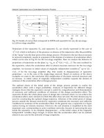
The evolution computed using (3) with , and has been
compared with the results of simulations where the approach described in the chapter is
applied. In Fig. 1 this comparison is reported, showing that (3) is a good model for
describing the relationship between the area covered and the time using a dynamic solution.

Fig. 1. Comparison between coverage evolution obtained by the model (2) (dashed) and
simulations of the proposed coverage strategy (solid) for different numbers of moving
sensors

Then, referring to surveillance tasks, (3) can be used to evaluate the minimum number of
sensors (with given and ) required to cover a given fraction of the area of
interest according to a given measurement rate. In fact, it is possible to write the relation
between the maximum rate at witch the network can cover the
fraction of and the
number of moving sensors as
New Developments in Robotics, Automation and Control

4

(4)

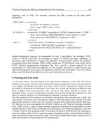
Such a relationship between and is depicted in Fig. 2, showing, as intuitively
expected, almost a proportionality between number of sensors and frequency of
measurement at each point of the area
.
The motivation and the support of the dynamic solution is evidenced by Fig. (1): lower
is the refresh frequency of the measurements at each point (that is higher are the time
intervals between measurements) and lower is the number of sensors required, once sensors
motion is introduced.

Fig. 2. Maximum measure rate
in function of number of moving sensors. ( ,
, , )

Under the assumption of dynamic network, the area coverage problem is posed in terms
of looking for optimal trajectories for the
moving sensors in presence of some constraints
like communication connection preservation, motion limitations, energetic considerations
and so on. In (Tsai et al., 2004, Cecil and Marthler, 2004) the dynamic coverage problem for
multiple sensors is studied , with a variational approach, in the level set framework,
obstacles occlusions are considered, suboptimal solutions are proposed also in three
dimensional environments ((Cecil and Marthler, 2006)). A survey of coverage path planning
algorithms for mobile robots moving on the plane is presented in (Choset, 2001). In (Acar et
al., 2006) the dynamic coverage problem for one mobile robot with finite range detectors is
studied and an approach based on space decomposition and Voronoy graphs is proposed.
In (Hussein and Stipanovic, 2007), a distributed control law is developed that guarantees to
meet the coverage goal with multiple mobile sensors under the hypothesis of
communication network connection. Collisions avoidance is considered.
The Area Coverage Problem for Dynamic Sensor Networks

5
Various problems associated with optimal path planning for mobile observers such as
mobile robots equipped with cameras to obtain maximum visual coverage in the three-
dimensional Euclidean space are considered in (Wang, 2003). Numerical algorithms for
solving the corresponding approximate problems are proposed.
In (Gabriele and Di Giamberardino, 2007c, Gabriele and Di Giamberardino, 2007a, Gabriele
and Di Giamberardino, 2007b) a general formulation of dynamic coverage is given by the
authors, a sensor network model is proposed and an optimal control formulation is given.
Suboptimal solutions are computed by discretization. Sensors and actuators limits,
geometric constraints, collisions avoidance, and communication network connectivity
maintenance are considered.
The approaches introduced up to now, also by the authors ((Gabriele and Di
Giamberardino, 2007c, Gabriele and Di Giamberardino, 2007a, Gabriele and Di
Giamberardino, 2007b)), are referred to homogeneous sensor networks, that is each node in
the network is equivalent to any other one in terms of sensing capabilities (same sensor or
same set of sensors over each node). Sensor network nodes were called heterogeneous with
respect to different aspects. In (Ling Lam and Hui Liu, 2007), the problem of deploying a set
of mobile sensor nodes, with heterogeneous sensing ranges, to give coverage is addressed.
In (Lazos and Poovendran, 2006), evaluating coverage of a set of sensors, with arbitrary
different shapes, deployed according to an arbitrary stochastic distribution is formulated as
a set intersection problem.
In (Hussein et al., 2007) the use of two classes of vehicles are used to dynamically cover a
given domain of interest. The first class is composed of vehicles, whose main responsibility
is to dynamically cover the domain of interest. The second class is composed of coordination
vehicles, whose main responsibility is to effectively communicate coverage information
across the network.
The problem of deploying nodes, equipped with different sets of sensors, is studied in (Shih
et al., 2007) in order to cover a sensing field in which multiple attributes are required to be
sensed.
In this chapter the case of different magnitudes to be measured on a given set of interest is

considered. Network nodes are then heterogeneous , like in (Shih et al., 2007), with respect
to the set of sensors with witch they are equipped. Moreover different sensors can have
different sensing ranges.

1.2 Connectivity Maintenance
Communication aspects are crucial in the design of a multi sensor systems ((Holger Karl,
2005, Stojmenovic, 2005, Santi, 2005)).
Connectivity is obviously necessary for data exchanging and aggregation but also for
localization and coordination, in fact, it is often assumed in formation stabilization (Olfati-
Saber and Murray, 2002) or consensus problems (Olfati-Saber et al., 2007).
In classical wireless sensor network (Holger Karl, 2005, Stojmenovic, 2005, Akyildiz et
al., 2002, Santi, 2005), composed by densely deployed static sensors, a single node has many
neighbours with which direct communication would be possible when using sufficiently
large transmission power. However high transmission power requires lots of energy, then, it
could be useful to deliberately restrict the set of neighbours controlling transmission power,
and then communication range, or by simply turning off some nodes for a certain time. For
such networks connectivity can then be achieved opportunely deploying nodes or
controlling communication power.
New Developments in Robotics, Automation and Control

6
For a dynamic sensor network the problem is more challenging, because network
topology is, indeed, dynamic. Connectivity maintenance became, then, a motion coordination
problem. Each sensor is assumed to have a fixed range over which communication is not
reliable. Communication network can be modelled as a state dependent dynamic graph;
topology, depending from sensors positions, changes while sensors moves.
Then, connectivity maintenance impose to introduce constrains on the instantaneous
positions of sensors. The simplest ways to achieve connectivity is to maintain the starting
communication graph topology that’s assumed to be connected. This can be obtained
imposing fixed topology Maintenance as proposed in (Gabriele and Di Giamberardino,

2007a) or flocking (Olfati-Saber, 2006). However, this approaches impose strong constraints
to sensors movement and that can affect other aspects as shown in (Gabriele and Di
Giamberardino, 2007b) for coverage. Is then more desirable to allow topology to change
over time, even though that introduce challenging dynamic graph control problems.
In (Mesbahi, 2004), starting from a class of problems associated with control of
distributed dynamic systems, a controllability framework for state-dependent dynamic
graphs is considered.
In (Kim and Mesbahi, 2005) the position of a dynamic state-dependent graph vertices are
controlled in order to maximize the second smallest eigenvalue of the Laplacian matrix, also
named algebraic connectivity and that has emerged as a critical parameter that influences the
stability and robustness properties of dynamic systems that operate over an information
network.
In (Spanos and Murray, 2004) a measure of robustness of local connectedness of a network is
introduced that can be computed by local communication only.
K-hop connectivity preservation is considered, in (Zavlanos, 2005), for a network with
dynamic nodes. A centralized control framework that guarantees maintenance of this
property is developed. Connectivity is modelled as an invariance problem and transformed
into a set of constraints on the control variable.
In (Gabriele and Di Giamberardino, 2007b) a centralized approach to connectivity
Maintenance, based on preservation of the edges of one Minimum Spanning Tree of the
communication graph, is proposed by the authors. Connection Maintenance is introduced as
a constraint of an optimization problem.

2. General Formulation

In this section definitions are given in order to introduce useful notations. A general model
of a dynamic sensor network is given considering heterogeneous sensors. The coverage
problem is formulated with respect to multiple magnitudes, connectivity maintenance
constraints are considered. In the following sections additional hypothesis are introduced in
order to simplify the general problem and to evaluate suboptimal solutions.

2.1 Dynamic Sensor networks
Let be
a specified spatial domain, a compact subset of the real Euclidean space
(n=2,3) called the set of interest. The representation of a point
with respect to a given
orthonormal basis for
is denoted by .
Let be
the set of magnitudes of interest defined on .
The Area Coverage Problem for Dynamic Sensor Networks

7
A dynamic sensor network can be view a set
of mobile sensors.
Each mobile sensor can be represented by:
where:
•
is the sensor configuration space.
•
is the sensor dynamic function, that describe the evolution of sensor
configuration according to a control input
:


•
is the set of magnitudes that sensor can measure.
• is the subset of within sensor , in configuration can
measure magnitude
. Let say that sensor in configuration

the set
•
is the sensor communication function, such as, in
configuration
can communicate with a sensor in configuration if and
only if
Looking at the whole network is possible to define generalized configuration and
generalized input as:



At the same manner the generalized dynamic of the whole network can be written as:




2.2 Coverage
Let indicate with the evolution of sensor configuration during a given a time
interval
. It is possible to define the subset of by during as:


(5)

New Developments in Robotics, Automation and Control

8
Considering generalized configuration
is possible to define the network field of
measure, respect to magnitude

during , as:


(6)

Looking at the whole magnitudes set, the subset of “ ” by the network
can be defined as:


(7)

The area by the sensor network during is then the measure of :


(8)


2.3 Communication
According with their communication capabilities sensors can be view as nodes of a dynamic
communication network. This network can be represented by a dynamic graph



where


indicate the nodes set and

indicate the edges set. As seen the edge set is time varying because it depends from the
network generalized configuration .
An alternative representation of the communication graph can be given using the adjacency
matrix
:



2.4 Area Coverage Problem
Making the sensor network to cover the set of interest means evaluating controls that drive
the network to measure the value of every magnitude on all the points of
, according with
some constrains.
Constrains can be due, for example, from:
• Limitation of sensors motion or measure rate
• Avoiding collisions between sensors
The Area Coverage Problem for Dynamic Sensor Networks

9
• Maintaining some communication networks features (topology, connectivity,…)

3. Dynamic Sensor Network Model

In this section the general model defined in 2 is specified adding the hypothesis of Linear
sensors dynamic, Proximity based measure model, Proximity based communication. Let
refer to this particular model as (LPP) Model.

3.1 Sensors Dynamics
Each sensor

is modelled, from the dynamic point of view, as a material point of mass
moving on
. The motion is assumed to satisfy the classical simple equations


(9)

where is the sensor position on . Sensor configuration is represented by:




The configuration space is then:



The linearity of 9 allows one to write the dynamics in the form


(10)

where





The evolutions of configuration (state) and position (output) are related with the input’s one
according with the well known equations:

(11)
New Developments in Robotics, Automation and Control

10
and


(12)

In the rest of the chapter sensor trajectory will refer to sensor position evolution.
Considering the whole network




can be defined to denote the generalized configuration, and the vector




to denote the generalized position that is represented, for each , by points in the
Euclidean space. Evolution of generalized position will be named generalized network
trajectory.
At the same manner the generalized input is defined as:




Generalized dynamics for the whole network can be written as:

where:






According with 11 and 12, generalized configuration evolution and network generalized
trajectory are related with generalized input by:
The Area Coverage Problem for Dynamic Sensor Networks

11

(13)

and


(14)

3.2 Coverage Model
It is assumed that at every time sensor can take measures on magnitude in a
circular area of radius
around its current position . The sensor field of measure
respect to
is then a disk of centre and radius :

(15)

As seen in 2.2, starting from is possible to define the area and the
area by the sensor network during a given time interval .
Homogeneous Sensors
A particular case is the one in witch sensors are homogeneous with respect to sensing
capabilities:




Assuming without loss of generality that there is only one magnitude of interest on ,
the set covered by sensor
at every time can be described by:


(16)

It is possible to define the subset of covered by the sensor network in a time interval
as:

(17)

New Developments in Robotics, Automation and Control

12
3.3 Communication Model
The communication network is modelled as an Euclidean graph. Two mobile sensors at time

are assumed to communicate each other if the distance between them is smaller than a
given communication radius
.
For every sensor
, the communication function is given by:


(18)


Is easy to see that this communication function makes the network graph undirected,
in fact:




3.4 Coverage Problem Formulation
According with the introduced model is possible to formulate the coverage problem as an
optimal control problem. The idea is to maximize the area covered by sensors in a fixed time
interval according with some constrains.

3.4.1 Objective Functional
In 2.2 the area by a set of moving sensors is defined as the union of the
measure sets of the sensors, respect to magnitude
, at every time . This quantity is very
hard to compute, also for the simple measure set model introduced in 3.2, then an
alternative performance measure has to be used.
Defining the distance between a point
of the workspace and a generalized trajectory
, within a time interval , as

(19)


and making use of the function


(20)


that fixes to zero any non positive value, the function




can be defined. Then, a measure of how the generalized trajectory produces a good
of the workspace can be given by
The Area Coverage Problem for Dynamic Sensor Networks

13

(21)


Looking at the whole magnitudes of interest set is possible to introduce a functional
that evaluate how a given generalized trajectory
the set of interest

(22)


Smaller is , better is the of . If then
completely the workspace.
From 3.1 is possible to see how
can be also written as:


(23)


Homogeneous Sensors
For the homogeneous sensors case the objective functional is:


(24)


3.4.2 Geometric Constraints
It is possible to constrain sensors to move inside a box subset of




If needed is possible to set the staring and/or the final state (positions and/or speeds):



A particular case is the periodic trajectories constrain, useful in tasks in which measures

have to be repeated continuously:




Is also necessary to avoid collisions between sensors at every time

New Developments in Robotics, Automation and Control

14


for

3.4.3 Dynamic Constraints
Physical limits on the actuators (for the motion) and/or on the sensors (in terms of velocity
in the measure acquisition) suggest the introduction of the following additional constraints




3.4.4 Communication Constraints
As said communication network connectivity is very important for data exchange and
transmission, but also for sensor localization, coordination and commands communication.
Under the hypothesis that before sensors start moving the communication network is
connected, it is possible to maintain connectivity introducing constraints on the
instantaneous position of sensors. More strongly, it is possible to impose a fixed network
topology, this can be useful, for example, to fix the level of redundancy on the
communication link an then to reach node fault tolerance.

Fixed Network Topology
To maintain a fixed network topology every sensor must maintain direct communication
with a subset of its starting neighbors that is fixed in time. Indicating with
the graph that represents desired topology, where
.
According with 3.3, for every edge of
a distance constrain between a couple of
sensors must be introduced, so maintaining a desired topology
means to satisfy the
following constrains set
:


(25)


Network Connectivity Maintenance
Fixed topology maintenance is, obviously a particular case of connectivity maintenance if
the desired topology is connected. Anyway, this approach introduces strong constrains on
sensors motion. This constrains can be relaxed in only connectivity is needed, allowing
network topology to change over time. That increase coverage performances as shown in
(Gabriele and Di Giamberardino, 2007b).
As said before, the communication model introduced in 3.3 makes the communication
graph
to be undirected. A undirected graph is connected if and only if it contain a
spanning tree. So it is possible to maintain network connectivity constraining every sensor
just to maintain direct communication links that corresponds to the edges of a spanning tree
of the communication tree.
The Area Coverage Problem for Dynamic Sensor Networks

15

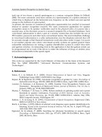
Fig. 3. Minimum Spanning Tree for a planar weighted undirected graph.

Assigning a weight at every edge of is possible to define the Minimum Spanning Tree
of
as the spanning tree with minimum weight (Figure 3). In particular being an
Euclidean graph it come natural to define the edges weights as:



in this case the minimum spanning tree is said Euclidean (EMST). The EMST can be easily
and efficiently computed by standard algorithms (such as Prim’s algorithm or Kruskal’s
algorithm). Indicating the EMST with
, where ,
maintaining the communication network connection means to satisfy the following
constrains
:


(26)


The minimum spanning tree of the communication network graph changes while
sensors moves, so the neighbours set of every node change over time making the network
topology dynamic.

3.4.5 Optimal Control Problem
The coverage problem can now be formulated as an optimal control problem:
New Developments in Robotics, Automation and Control

16


This problem is, in general, very hard to solve analytically. In the next section a simpler
discretized model is introduced to evaluate suboptimal solutions.

4. Discretized Model

In order to overcome the difficulty of the problem defined in 3.4, a discretization is
performed, both with respect to space, and with respect to time in all the time dependent
expressions. The workspace
is then divided into square cells, with resolution (size) ,
obtaining a grid in witch each point
is the centre of a cell, and the trajectories are
discretized with sample time
. This allow to represent the coverage problem as a solvable
Nonlinear Programming Problem .

4.1 Sensors Discretized Dynamics
The discrete time sensors dynamic is well described by the following equations:


(27)


where

Representing the sensor input sequence from time to time as:
The Area Coverage Problem for Dynamic Sensor Networks

17



and defining the following vectors



is possible to write state and output values at time as:


(28)


and


(29)


State and output sequences, from time to time , can be represented by the
following vectors:




According with 28 and 29 the relations between these sequences and the input one are

described by: