The Materials Information Company.Publication Information and alloy phase diagrams volume 3 pot
Bạn đang xem bản rút gọn của tài liệu. Xem và tải ngay bản đầy đủ của tài liệu tại đây (33.19 MB, 1,741 trang )
ASM
INTERNATIONAL ®
The Materials
Information Company
Publication Information and Contributors
Alloy Phase Diagrams was published in 1992 as Volume 3 of the ASM Handbook. The Volume was prepared under the
direction of the ASM International Alloy Phase Diagram and the Handbook Committees.
Foreword
Phase diagrams, thermodynamic data in graphical form, are one of the basic tools of the metallurgist, materials scientist,
and materials engineer. They can be used for alloy design, selection of hot-working and fabricating parameters, prediction
of performance, guidance in selection of hot-working and fabricating parameters, prediction of performance, guidance in
selection of heat-treating process parameters, solving performance problems, including failure analysis, and for many
other purposes.
The formation of The American Society of Steel Treating, the forerunner of ASM International, was based on better
understanding of heat-treating technology; this understanding was, of course, rooted in part in the proper utilization of
phase diagrams. Experimental tools such as metallography were used in those early days, both to determine phase
diagrams and to link the heat-treating process with the desired microstructure.
In 1978 ASM International joined with the National Bureau of Standards (now the National Institute of Standards of
Technology, or NIST) in an effort to improve the reliability of phase diagrams by evaluating the existing data on a
system-by-system basis. ASM raised $4 million from industry and government sources and NIST provided a similar
amount of financial and in-kind support for this historic undertaking. An international effort was mounted simultaneously
with similar objectives. As a result, all of the important binary systems have been evaluated, and international partners
have evaluated more than 2000 ternary systems.
ASM actively participates in the Alloy Phase Diagram International Commission (APDIC), which comprises cooperative
national or regional committees in 13 countries. APDIC was formed "to set overall objectives, determine priorities for
alloy systems to be assessed, coordinate the assessment programs of APDIC members and associate members, establish
scope and quality standards for assessment programs in other countries, and assist in the timely dissemination of the
resultant phase diagram data."
The complete results of the international effort are recorded in various periodical and reference publications. However,
we have continued to hear from ASM members that a summary version consisting primarily of phase diagrams should be
published as an ASM Handbook for the practicing engineer. While such a Handbook could not contain all the diagrams
and data, careful selection would ensure the inclusion of the most important systems, with references to other more
complete sources. The present Handbook is the result of our attempts to meet these criteria and the stated need.
No reference book of this nature could be published without the contributions of literally hundreds of technical and staff
workers. On behalf of ASM International, we extend our sincere thanks and appreciation to the category editors,
contributors, reviewers, and staff who worked in this international effort. Thanks are also due to the ASM Alloy Phase
Diagram and Handbook Committees for their guidance and support of the project.
• Edward H. Kottcamp, Jr.
President
ASM International
• Edward L. Langer
Managing Director
ASM International
Preface
Alloy phase diagrams have long been used successfully by the scientific, engineering, and industrial communities as
"road maps" to solve a variety of practical problems. It is, thus, not surprising that such diagrams have always been an
important part of ASM Handbooks. The previous ASM compilation of commercially important diagrams appeared in
Volume 8 of the 8th Edition of Metals Handbook.
Shortly after publication of the earlier volume in 1973, recognition of the universal importance of alloy phase diagrams
led to the formation of several national phase diagram programs, as well as the International Programme for Alloy Phase
Diagrams to act as the coordinating body for these activities. In the U. S., the national program has been spearheaded
jointly by ASM International and the National Institute of Standards and Technology.
To meet the pressing need for diagrams, the national programs and the entire International Programme had two main
goals: to increase the availability of phase diagrams and to ensure that the diagrams made available were of the highest
possible quality. The specific tasks that were undertaken to accomplish these goals included assembling all existing data
related to alloy phase diagrams, critically evaluating these data, using the data to construct the most up-to-date and
accurate diagrams possible, and making the resulting diagrams readily available for use.
With the publication of the three-volume set of Binary Alloy Phase Diagrams, Second Edition, by ASM in 1991, the
binary alloy portion of this monumental task is virtually complete. In addition, the first-ever truly comprehensive
collection of ternary diagrams, the multivolume Handbook of Ternary Alloy Phase Diagrams, is scheduled for publication
by ASM in 1994. Information from these two extensive and current diagram sources have been used as the basis of this
updated engineering reference book, which reproduces the diagrams of the most commercially important systems (1046
binaries plus 80 ternaries) in a single, convenient volume. These alloy systems are represented by more than 1100 binary
diagrams and 313 ternary diagrams, all plotted in weight percent as the primary scale.
The binary diagrams reproduced in this Handbook were selected from the 2965 systems covered in Binary Alloy Phase
Diagrams, with updated diagrams from literature published since January 1991. Included with the binary diagrams is a
complete index of all known alloy phase diagrams from all sources, listing where each can be found should a problem
arise concerning a binary system not covered in this Handbook. Although many of the diagrams listed in this index (and a
few of those reproduced in this volume) have not been evaluated under the Programmed, they were selected to represent
the best available. Updated binary diagrams from the phase diagram update section of the Journal of Phase Equilibria and
abstracts of new full-length evaluation from the Journal of Phase Equilibria and the Monograph Series on Alloy Phase
Diagrams are available from ASM International on a continuing basis through the Binary Alloy Phase Diagrams Updating
Service.
The ternary diagrams reproduced here were selected from more than 12,000 diagrams being assembled for the ternary
handbook. Where available, diagrams from recently published evaluated compilations were selected. The remainder were
selected to represent the best available.
To aid in the full and effective use of these diagrams to solve practical problems, we have included an Introduction to
Alloy Phase Diagrams, which contains sections on the theory and use of phase diagrams, and an Appendix listing the
relevant properties of the elements and their crystal structures.
While the work of developing additional data, expanding alloy system coverage, and refining existing diagrams must and
will continue, the quality checks built into the programme ensure that the diagrams reproduced here are as accurate and
reliable as possible. Credit for this belongs to the conscientious work of all the experts involved in the worldwide
Programme, especially Prof. Thaddeus B. Massalski and Dr. Alan A. Prince, who coordinated the evaluation efforts
during the period of greatest activity.
The Editors
General Information
Officers and Trustees of ASM International
Officers
• LAMET UFRGS
• Edward H. Kottcamp, Jr. President and Trustee SPS Technologies
• John G. Simon Vice President and Trustee General Motors Corporation
• William P. Koster Immediate Past President Metcut Research Associates, Inc.
• Edward L. Langer Secretary and Managing Director ASM International
• Leo G. Thompson Treasurer Lindberg Corporation
Trustees
• William H. Erickson Canada Centre for Minerals & Energy
• Norman A. Gjostein Ford Motor Company
• Nicholas C. Jessen, Jr. Martin Marietta Energy Systems, Inc.
• E. George Kendall Northrop Aircraft
• George Krauss Colorado School of Mines
• Gernant E. Maurer Special Metals Corporation
• Alton D. Romig, Jr. Sandia National Laboratories
• Lyle H. Schwartz National Institute of Standards & Technology (NIST)
• Merle L. Thorpe Hobart Tafa Technologies, Inc.
Members of the ASM Alloy Phase Diagram Committee (1991-1992)
• Michael R. Notis (Chairman 1991-; Member 1988-) Lehigh University
• James Brown (1990-) Ontario Hydro
• Cathleen M. Cotell (1991-) Naval Research Labs
• Charles E. Ells (1991-) Atomic Energy of Canada, Ltd.
• Gretchen Kalonji (1991-) University of Washington
• Marc H. LaBranche (1991-) DuPont
• Vincent C. Marcotte (1987-) IBM East Fishkill Facility
• T.B. Massalski (1987-) Carnegie-Mellon University
• Sailesh M. Merchant (1990-) AT&T Bell Labs
• John E. Morral (1990-) University of Connecticut
• Charles A. Parker (1987-) Allied Signal Research & Technology
• Alan Prince (1987-) Consultant
• Gaylord D. Smith (1987-) Inco Alloys International Inc.
• Michael S. Zedalis (1991-) Allied Signal, Inc.
Members of the ASM Handbook Committee (1992-1993)
• Roger J. Austin (Chairman 1992-; Member 1984-) Hydro-Lift
• David V. Neff (Vice-Chairman 1992-; Member 1986-) Metaullics System
• Ted Anderson (1991-) Texas A&M University
• Bruce Bardes (1992-) GE Aircraft Engines
• Robert J. Barnhurst (1988-) Noranda Technology Centre
• Toni Brugger (1992-) Phoenix Pipe & Tube Co.
• Stephen J. Burden (1989-) GTE Valenite
• Craig V. Darragh (1989-) The Timken Company
• Russell J. Diefendorf (1990-) Clemson University
• Aicha Elshabini-Riad (1990-) Virginia Polytechnic & State University
• Gregory A. Fett (1992-) Dana Corporation
• Michelle M. Gauthier Raytheon Company
• Toni Grobstein (1990-) NASA Lewis Research Center
• Susan Housh (1990-) Dow Chemical U.S.A.
• Dennis D. Huffman (1982-) The Timken Company
• S. Jim Ibarra (1991-) Amoco Research Center
• J. Ernesto Indacochea (1987-) University of Illinois at Chicago
• Peter W. Lee (1990-) The Timken Company
• William L. Mankins (1989-) Inco Alloys International, Inc.
• Richard E. Robertson (1990-) University of Michigan
• Jogender Singh (1992-) NASA
• Jeremy C. St. Pierre (1990-) Hayes Heat Treating Corporation
• Ephraim Suhir (1990-) AT&T Bell Laboratories
• Kenneth B. Tator (1991-) KTA-Tator, Inc.
• Malcolm Thomas (1992-) General Motors Corp.
• William B. Young (1991-) Dana Corporation
Staff
ASM International staff who contributed to the development of the Volume included Hugh Baker, Editor; Hiroaki
Okamoto, Senior Technical Editor; Scott D. Henry, Manager of Handbook Development; Grace M. Davidson, Manager,
Production Systems; Mary Anne Fleming, Manager, APD Publications; Linda Kacprzak, Manager of Production; Heather
F. Lampman, Editorial/Production Assistant; William W. Scott, Jr., Technical Director; Robert C. Uhl, Director of
Reference Publications. Editorial Assistance was provided by Nikki D. Wheaton and Kathleen Mills. Production
Assistance was provided by Donna Sue Plickert, Steve Starr, Karen Skiba, Patricia Eland, and Jeff Fenstermaker.
Conversion to Electronic Files
ASM Handbook, Volume 3, Alloy Phase Diagrams was converted to electronic files in 1998. The conversion was based
on the First Printing (1992). No substantive changes were made to the content of the Volume, but some minor corrections
and clarifications were made as needed.
ASM International staff who contributed to the conversion of the Volume included Sally Fahrenholz-Mann, Bonnie
Sanders, Marlene Seuffert, Scott Henry, and Robert Braddock. The electronic version was prepared under the direction of
William W. Scott, Jr., Technical Director, and Michael J. DeHaemer, Managing Director.
Copyright Information (for Print Volume)
Copyright © 1992 by ASM International
All rights reserved
No part of this book may be reproduced, stored in a retrieval system, or transmitted, in any form or by any means,
electronic, mechanical, photocopying, recording, or otherwise, without the written permission of the copyright owner.
ASM Handbook is a collective effort involving thousands of technical specialists. It brings together in one book a wealth
of information from world-wide sources to help scientists, engineers, and technicians solve current and long-range
problems.
Great care is taken in the compilation and production of this Volume, but it should be made clear that NO
WARRANTIES, EXPRESS OR IMPLIED, INCLUDING, WITHOUT LIMITATION, WARRANTIES OF
MERCHANTABILITY OR FITNESS FOR A PARTICULAR PURPOSE, ARE GIVEN IN CONNECTION WITH
THIS PUBLICATION. Although this information is believed to be accurate by ASM, ASM cannot guarantee that
favorable results will be obtained from the use of this publication alone. This publication is intended for use by persons
having technical skill, at their sole discretion and risk. Since the conditions of product or material use are outside of
ASM's control, ASM assumes no liability or obligation in connection with any use of this information. No claim of any
kind, whether as to products or information in this publication, and whether or not based on negligence, shall be greater in
amount than the purchase price of this product or publication in respect of which damages are claimed. THE REMEDY
HEREBY PROVIDED SHALL BE THE EXCLUSIVE AND SOLE REMEDY OR BUYER, AND IN NO EVENT
SHALL EITHER PARTY BE LIABLE FOR SPECIAL, INDIRECT OR CONSEQUENTIAL DAMAGES WHETHER
OR NOT CAUSED BY OR RESULTING FROM THE NEGLIGENCE OF SUCH PARTY. As with any material,
evaluation of the material under end-use conditions prior to specification is essential. Therefore, specific testing under
actual conditions is recommended.
Nothing contained in this book shall be construed as a grant of any right of manufacture, sale, use, or reproduction, in
connection with any method, process, apparatus, product, composition, or system, whether or not covered by letters
patent, copyright, or trademark, and nothing contained in this book shall be construed as a defense against any alleged
infringement of letters patent, copyright, or trademark, or as a defense against liability for such infringement.
Comments, criticisms, and suggestions are invited, and should be forwarded to ASM International.
Library of Congress Cataloging-in-Publication Data (for Print Volume)
ASM handbook.
(Revised for vol. 3)
Vols. 1-2 have title: Metals handbook. Includes biographical references and indexes. Contents: v. 1. Properties and
selection irons, steels, and high-performance alloys v. 2. Properties and selection nonferrous alloys and special-
purpose v. 3. Alloy phase diagrams
1. Metals Handbooks, manuals, etc.
I. ASM International. Handbook Committee
II. Metals handbook.
TA459.M43 1990 620.1'6 90-115
ISBN: 0-87170-377-7 (v.1) 0-87170-381-5 (v.3)
SAN: 204-7586
Printed in the United States of America
Introduction to Alloy Phase Diagrams
Hugh Baker, Editor
Introduction
ALLOY PHASE DIAGRAMS are useful to metallurgists, materials engineers, and materials scientists in four major
areas: (1) development of new alloys for specific applications, (2) fabrication of these alloys into useful configurations,
(3) design and control of heat treatment procedures for specific alloys that will produce the required mechanical, physical,
and chemical properties, and (4) solving problems that arise with specific alloys in their performance in commercial
applications, thus improving product predictability. In all these areas, the use of phase diagrams allows research,
development, and production to be done more efficiently and cost effectively.
In the area of alloy development, phase diagrams have proved invaluable for tailoring existing alloys to avoid overdesign
in current applications, designing improved alloys for existing and new applications, designing special alloys for special
applications, and developing alternative alloys or alloys with substitute alloying elements to replace those containing
scarce, expensive, hazardous, or "critical" alloying elements. Application of alloy phase diagrams in processing includes
their use to select proper parameters for working ingots, blooms, and billets, finding causes and cures for microporosity
and cracks in castings and welds, controlling solution heat treating to prevent damage caused by incipient melting, and
developing new processing technology.
In the area of performance, phase diagrams give an indication of which phases are thermodynamically stable in an alloy
and can be expected to be present over a long time when the part is subjected to a particular temperature (e.g., in an
automotive exhaust system). Phase diagrams also are consulted when attacking service problems such as pitting and
intergranular corrosion, hydrogen damage, and hot corrosion.
In a majority of the more widely used commercial alloys, the allowable composition range encompasses only a small
portion of the relevant phase diagram. The nonequilibrium conditions that are usually encountered in practice, however,
necessitate the knowledge of a much greater portion of the diagram. Therefore, a thorough understanding of alloy phase
diagrams in general and their practical use will prove to be of great help to a metallurgist expected to solve problems in
any of the areas mentioned above.
Common Terms
Before the subject of alloy phase diagrams is discussed in detail, several of the commonly used terms will be discussed.
Phases. All materials exist in gaseous liquid, or solid form (usually referred to as a phase), depending on the conditions
of state. State variables include composition, temperature, pressure, magnetic field, electrostatic field, gravitational field,
and so on. The term "phase" refers to that region of space occupied by a physically homogeneous material. However,
there are two uses of the term: the strict sense normally used by physical scientists and the somewhat looser sense
normally used by materials engineers.
In the strictest sense, homogeneous means that the physical properties throughout the region of space occupied by the
phase are absolutely identical, and any change in condition of state, no matter how small, will result in a different phase.
For example, a sample of solid metal with an apparently homogeneous appearance is not truly a single-phase material,
because the pressure condition varies in the sample due to its own weight in the gravitational field.
In a phase diagram, however, each single-phase field (phase fields are discussed in a following section) is usually given a
single label, and engineers often find it convenient to use this label to refer to all the materials lying within the field,
regardless of how much the physical properties of the materials continuously change from one part of the field to another.
This means that in engineering practice, the distinction between the terms "phase" and "phase field" is seldom made, and
all materials having the same phase name are referred to as the same phase.
Equilibrium. There are three types of equilibia: stable, metastable, and unstable. These three conditions are illustrated in
a mechanical sense in Fig. 1. Stable equilibrium exists when the object is in its lowest energy condition; metastable
equilibrium exists when additional energy must be introduced before the object can reach true stability; unstable
equilibrium exists when no additional energy is needed before reaching metastability or stability. Although true stable
equilibrium conditions seldom exist in metal objects, the study of equilibrium systems is extremely valuable, because it
constitutes a limiting condition from which actual conditions can be estimated.
Fig. 1 Mechanical equilibria: (a) Stable. (b) Metastable. (c) Unstable
Polymorphism. The structure of solid elements and compounds under stable equilibrium conditions is crystalline, and
the crystal structure of each is unique. Some elements and compounds, however, are polymorphic (multishaped); that is,
their structure transforms from one crystal structure to another with changes in temperature and pressure, each unique
structure constituting a distinctively separate phase. The term allotropy (existing in another form) is usually used to
describe polymorphic changes in chemical elements. Crystal structure of metals and alloys is discussed in a later section
of this Introduction; the allotropic transformations of the elements are listed in the Appendix to this Volume.
Metastable Phases. Under some conditions, metastable crystal structures can form instead of stable structures. Rapid
freezing is a common method of producing metastable structures, but some (such as Fe
3
C, or "cementite") are produced at
moderately slow cooling rates. With extremely rapid freezing, even thermodynamically unstable structures (such as
amorphous metal "glasses") can be produced.
Systems. A physical system consists of a substance (or a group of substances) that is isolated from its surroundings, a
concept used to facilitate study of the effects of conditions of state. "Isolated" means that there is no interchange of mass
between the substance and its surroundings. The substances in alloy systems, for example, might be two metals, such as
copper and zinc; a metal and a nonmetal, such as iron and carbon; a metal and an intermetallic compound, such as iron
and cementite; or several metals, such as aluminum, magnesium, and manganese. These substances constitute the
components comprising the system and should not be confused with the various phases found within the system. A
system, however, also can consist of a single component, such as an element or compound.
Phase Diagrams. In order to record and visualize the results of studying the effects of state variables on a system,
diagrams were devised to show the relationships between the various phases that appear within the system under
equilibrium conditions. As such, the diagrams are variously called constitutional diagrams, equilibrium diagrams, or
phase diagrams. A single-component phase diagram can be simply a one- or two-dimensional plot showing the phase
changes in the substance as temperature and/or pressure change. Most diagrams, however, are two- or three-dimensional
plots describing the phase relationships in systems made up of two or more components, and these usually contain fields
(areas) consisting of mixed-phase fields, as well as single-phase fields. The plotting schemes in common use are
described in greater detail in subsequent sections of this Introduction.
System Components. Phase diagrams and the systems they describe are often classified and named for the number (in
Latin) of components in the system:
Number of
components
Name of
system or diagram
One Unary
Two Binary
Three Temary
Four Quaternary
Five Quinary
Six Sexinary
Seven Septenary
Eight Octanary
Nine Nonary
Ten Decinary
Phase Rule. The phase rule, first announced by J. William Gibbs in 1876, related the physical state of a mixture to the
number of constituents in the system and to its conditions. It was also Gibbs who first called each homogeneous region in
a system by the term "phase." When pressure and temperature are the state variables, the rule can be written as follows:
f = c - p + 2
where f is the number of independent variables (called degrees of freedom), c is the number of components, and p is the
number of stable phases in the system.
Unary Diagrams
Invariant Equilibrium. According to the phase rule, three phases can exist in stable equilibrium only at a single point
on a unary diagram (f = 1 - 3 + 2 = 0). This limitation is illustrated as point O in the hypothetical unary pressure-
temperature (PT) diagram shown in Fig. 2. In this diagram, the three states (or phases) solid, liquid, and gas are
represented by the three correspondingly labeled fields. Stable equilibrium between any two phases occurs along their
mutual boundary, and invariant equilibrium among all three phases occurs at the so-called triple point, O, where the three
boundaries intersect. This point also is called an invariant point because, at that location on the diagram, all externally
controllable factors are fixed (no degrees of freedom). At this point, all three states (phases) are in equilibrium, but any
changes in pressure and/or temperature will cause one or two of the states (phases) to disappear.
Fig. 2 Schematic pressure-temperature phase diagram
Univariant Equilibrium The phase rule says that stable equilibrium between two phases in a unary system allows one
degree of freedom (f = 1 - 2 + 2). This condition, called univariant equilibrium or monovariant equilibrium, is illustrated
as line 1, 2, and 3 separating the single-phase fields in Fig. 2. Either pressure or temperature may be freely selected, but
not both. Once a pressure is selected, there is only one temperature that will satisfy equilibrium conditions, and
conversely. The three curves that issue from the triple point are called triple curves: line 1, representing the reaction
between the solid and the gas phases, is the sublimation curve; line 2 is the melting curve; and line 3 is the vaporization
curve. The vaporization curve ends at point 4, called a critical point, where the physical distinction between the liquid and
gas phase disappears.
Bivariant Equilibrium. If both the pressure and temperature in a unary system are freely and arbitrarily selected, the
situation corresponds to having two degrees of freedom, and the phase rule says that only one phase can exit in stable
equilibrium (p = 1 - 2 + 2). This situation is called bivariant equilibrium.
Binary Diagrams
If the system being considered comprises two components, a composition axis must be added to the PT plot, requiring
construction of a three-dimensional graph. Most metallurgical problems, however, are concerned only with a fixed
pressure of one atmosphere, and the graph reduces to a two-dimensional plot of temperature and composition (TX
diagram).
The Gibbs phase rule applies to all states of matter (solid, liquid, and gaseous), but when the effect of pressure is constant,
the rule reduces to:
f = c - p + 1
The stable equilibria for binary systems are summarized as follows:
Number of
components
Number of
phases
Degrees of
freedom
Equilibrium
2 3 0 Invariant
2 2 1 Univariant
2 1 2 Bivariant
Miscible Solids. Many systems are comprised of components having the same crystal structure, and the components of
some of these systems are completely miscible (completely soluble in each other) in the solid form, thus forming a
continuous solid solution. When this occurs in a binary system, the phase diagram usually has the general appearance of
that shown in Fig. 3. The diagram consists of two single-phase fields separated by a two-phase field. The boundary
between the liquid field and the two-phase field in Fig. 3 is called the liquidus; that between the two-phase field and the
solid field is the solidus. In general, a liquidus is the locus of points in a phase diagram representing the temperatures at
which alloys of the various compositing of the system begin to freeze on cooling or finish melting on heating; a solidus is
the locus of points representing the temperatures at which the various alloys finish freezing on cooling or begin melting
on heating. The phases in equilibrium across the two-phase field in Fig. 3 (the liquid and solid solutions) are called
conjugate phases.
Fig. 3 Schematic binary phase diagram showing miscibility in both the liquid and solid states
If the solidus and liquids meet tangentially at some point, a maximum or minimum is produced in the two-phase field,
splitting it into two portions as shown in Fig. 4. It also is possible to have a gap in miscibility in a single-phase field; this
is show in Fig. 5 Point T
c
, above which phases α
1
and α
2
become indistinguishable, is a critical point similar to point 4 in
Fig. 2. Lines a-T
c
and b-T
c
, called solvus lines, indicate the limits of solubility of component B in A and A in B,
respectively. The configurations of these and all other phase diagrams depend on the thermodynamics of the system, as
discussed later in this Introduction.
Fig. 4 Schematic binary phase diagrams with solid-
state miscibility where the liquidus shows a maximum (a)
and a minimum (b)
Fig. 5 Schematic binary phase diagram with a minimum in the liquidus and a miscibility gap in the solid state
Eutectic Reactions. If the two-phase field in the solid region of Fig. 5 is expanded so that it touches the solidus at
some point, as shown in Fig. 6(a), complete miscibility of the components is lost. Instead of a single solid phase, the
diagram now shows two separate solid terminal phases, which are in three-phase equilibrium with the liquid at point P, an
invariant point that occurred by coincidence. (Three-phase equilibrium is discussed in the following section.) Then, if this
two-phase field in the solid region is even further widened so that the solvus lines no longer touch at the invariant point,
the diagram passes through a series of configurations, finally taking on the more familiar shape shown in Fig. 6(b). The
three-phase reaction that takes place at the invariant point E, where a liquid phases, freezes into a mixture of two solid
phases, is called a eutectic reaction (from the Greek word for "easily melted"). The alloy that corresponds to the eutectic
composition is called a eutectic alloy. An alloy having a composition to the left of the eutectic point is called a
hypoeutectic alloy (from the Greek word for "less than"); an alloy to the right is a hypereutectic alloy (meaning "greater
than").
Fig. 6 Schematic binary phase diagrams with invariant points. (a) Hypothetical diagr
am of the type shown in
Fig. 5, except that the miscibility gap in the solid touches the solidus curve at invariant po
int P; an actual
diagram of this type probably does not exist. (b) and (c) Typical eutectic diagrams for components having the
same crystal structure (b) and components having different crystal structures (c); the eutectic (invariant)
points are labeled E. The dashed lines in (b) and (c) are metastable extensions of the stable-equilibria lines.
In the eutectic system described above, the two components of the system have the same crystal structure. This, and other
factors, allows complete miscibility between them. Eutectic systems, however, also can be formed by two components
having different crystal structures. When this occurs, the liquidus and solidus curves (and their extensions into the two-
phase field) for each of the terminal phases (see Fig. 6c) resemble those for the situation of complete miscibility between
system components shown in Fig. 3.
Three-Phase Equilibrium. Reactions involving three conjugate phases are not limited to the eutectic reaction. For
example, upon cooling, a single solid phase can change into a mixture of two new solid phases or, conversely, two solid
phases can react to form a single new phase. These and the other various types of invariant reactions observed in binary
systems are listed in Table 1 and illustrated in Fig. 7 and 8.
Table 1 Invariant reactions
Fig. 7 Hypothetical binary phase diagram s
howing intermediate phases formed by various invariant reactions
and a polymorphic transformation
Fig. 8 Hypothetical binary
phase diagram showing three intermetallic line compounds and four melting
reactions
Intermediate Phases. In addition to the three solid terminal-phase fields, α, β, and ε, the diagram in Fig. 7 displays
five other solid-phase fields, γ, δ, δ', η, and σ, at intermediate compositions. Such phases are called intermediate phases.
Many intermediate phases, such as those illustrated in Fig. 7, have fairly wide ranges of homogeneity. However, many
others have very limited or no significant homogeneity range.
When an intermediate phase of limited (or no) homogeneity range is located at or near a specific ratio of component
elements that reflects the normal positioning of the component atoms in the crystal structure of the phase, it is often called
a compound (or line compound). When the components of the system are metallic, such an intermediate phase is often
called an intermetallic compound. (Intermetallic compounds should not be confused with chemical compounds, where the
type of bonding is different from that in crystals and where the ratio has chemical significance.) Three intermetallic
compounds (with four types of melting reactions) are shown in Fig. 8.
In the hypothetical diagram shown in Fig. 8, an alloy of composition AB will freeze and melt isothermally, without the
liquid of solid phases undergoing changes in composition; such a phase change is called congruent. All other reactions are
incongruent; that is, two phases are formed from one phase on melting. Congruent and incongruent phase changes,
however, are not limited to line compounds: the terminal component B (pure phase ε) and the highest-melting
composition of intermediate phase δ' in Fig. 7, for example, freeze and melt congruently, while δ' and ε freeze and melt
incongruently at other compositions.
Metastable Equilibrium. In Fig. 6(c), dashed lines indicate the portions of the liquidus and solidus lines that disappear
into the two-phase solid region. These dashed lines represent valuable information, as they indicate conditions that would
exist under metastable equilibrium, such as might theoretically occur during extremely rapid cooling. Metastable
extensions of some stable-equilibria lines also appear in Fig. 2 and 6(b).
Ternary Diagrams
When a third component is added to a binary system, illustrating equilibrium conditions in two dimensions becomes more
complicated. One option is to add a third composition dimension to the base, forming a solid diagram having binary
diagrams as its vertical sides. This can be represented as a modified isometric projection, such as shown in Fig. 9. Here,
boundaries of single-phase fields (liquidus, solidus, and solvus lines in the binary diagrams) become surfaces; single- and
two-phase areas become volumes; three-phase lines become volumes; and four-phase points, while not shown in Fig. 9,
can exist as an invariant plane. The composition of a binary eutectic liquid, which is a point in a two-component system,
becomes a line in a ternary diagram, as shown in Fig. 9.
Fig. 9 Ternary phase diagram showing three-phase equilibrium. Source: 56Rhi 3
Although three-dimensional projections can be helpful in understanding the relationship in a diagram, reading values
from them is difficult. Therefore, ternary systems are often represented by views of the binary diagrams that comprise the
faces and two-dimensional projections of the liquidus and solidus surfaces, along with a series of two-dimensional
horizontal sections (isotherms) and vertical sections (isopleths) through the solid diagram.
Vertical sections are often taken through one corner (one component) and a congruently melting binary compound that
appears on the opposite face; when such a plot can be read like any other true binary diagram, it is called a quasibinary
section. One possibility is illustrated by line 1-2 in the isothermal section shown in Fig. 10. A vertical section between a
congruently melting binary compound on one face and one on a different face might also form a quasibinary section (see
line 2-3).
Fig. 10 Isothermal section of a ternary diagram with phase boundaries deleted for simplification.
All other vertical sections are not true binary diagrams, and the term pseudobinary is applied to them. A common
pseudobinary section is one where the percentage of one of the components is held constant (the section is parallel to one
of the faces), as shown by line 4-5 in Fig. 10. Another is one where the ratio of two constituents is held constant and the
amount of the third is varied from 0 to 100% (line 1-5).
Isothermal Sections. Composition values in the triangular isothermal sections are read from a triangular grid
consisting of three sets of lines parallel to the faces and placed at regular composition intervals (see Fig. 11). Normally,
the point of the triangle is placed at the top of the illustration, component A is placed at the bottom left, B at the bottom
right, and C at the top. The amount of component A is normally indicated from point C to point A, the amount of
component B from point A to point B, and the amount of component C from point B to point C. This scale arrangement is
often modified when only a corner area of the diagram is shown.
Fig. 11 Triangular
composition grid for isothermal section; x is the composition of each constituent in mole
fraction or percent.
Projected Views. Liquidus, solids, and solvus surfaces by their nature are not isothermal. Therefore, equal-temperature
(isothermal) contour lines are often added to the projected views of these surfaces to indicate their shape (see Fig. 12). In
addition to (or instead of) contour lines, views often show lines indicating the temperature troughs (also called "valleys"
or "grooves") formed at the intersections of two surfaces. Arrowheads are often added to these lines to indicate the
direction of decreasing temperature in the trough.
Fig. 12 Liquidus projection of a ternary phase diagram showing isothermal contour lines. Source: Adapted f
rom
56Rhi 3
Reference cited in this section
3.
56Rhi: F.N. Rhines, Phase Diagrams in Metallurgy: Their Development and Application, McGraw-
Hill,
1956. This out-of-print book is a basic text designed for undergraduate students in metallurgy.
Thermodynamic Principles
The reactions between components, the phases formed in a system, and the shape of the resulting phase diagram can be
explained and understood through knowledge of the principles, laws, and terms of thermodynamic, and how they apply to
the system.
Internal Energy. The sum of the kinetic energy (energy of motion) and potential energy (stored energy) of a system is
called its internal energy, E. Internal energy is characterized solely by the state of the system.
Closed System. A thermodynamic system that undergoes no interchange of mass (material) with its surroundings is
called a closed system. A closed system, however, can interchange energy with its surroundings.
First Law. The First Law of Thermodynamics, as stated by Julius von Mayer, James Joule, and Hermann von Helmholtz
in the 1840s, states that energy can be neither created nor destroyed. Therefore, it is called the Law of Conservation of
Energy. This law means that the total energy of an isolated system remains constant throughout any operations that are
carried out on it; that is, for any quantity of energy in one form that disappears from the system, an equal quantity of
another form (or other forms) will appear.
For example, consider a closed gaseous system to which a quantity of heat energy δQ, is added and a quantity of work,
δW, is extracted. The First Law describes the change in internal energy, dE, of the system as follows:
dE = δQ - δW
In the vast majority of industrial processes and material applications, the only work done by or on a system is limited to
pressure/volume terms. Any energy contributions from electric, magnetic, or gravitational fields are neglected, except for
electrowinning and electrorefining processes such as those used in the production of copper, aluminum, magnesium, the
alkaline metals, and the alkaline earths. With the neglect of field effects, the work done by a system can be measured by
summing the changes in volume, dV, times each pressure causing a change. Therefore, when field effects are neglected,
the First Law can be written:
dE =δQ - PdV
Enthalpy. Thermal energy changes under constant pressure (again neglecting any field effects) are most conveniently
expressed in terms of the enthalpy, H, of a system. Enthalpy, also called heat content, is defined by:
H = E + PV
Enthalpy, like internal energy, is a function of the state of the system, as is the product PV.
Heat Capacity. The heat capacity, C, of a substance is the amount of heat required to raise its temperature one degree;
that is:
However, if the substance is kept at constant volume (dV = 0):
δQ = dE
and
If, instead, the substance is kept at constant pressure (as in many metallurgical systems),
and
Second Law. While the First Law establishes the relationship between the heat absorbed and the work performed by a
system, it places no restriction on the source of the heat or its flow direction. This restriction, however, is set by the
Second Law of Thermodynamics, which was advanced by Rudolf Clausius and William Thomson (Lord Kelvin). The
Second Law states that the spontaneous flow of heat always is from the higher temperature body to the lower temperature
body. In other words, all naturally occurring processes tend to take place spontaneously in the direction that will lead to
equilibrium.
Entropy. The Second Law is not conveniently stated in terms of entropy, S, another property of state possessed by all
systems. Entropy represents the energy (per degree of absolute temperature, T) in a system that is not available for work.
In terms of entropy, the Second Law states that all natural processes tend to occur only with an increase in entropy, and
the direction of the process always is such as to lead to an increase in entropy. For processes taking place in a system in
equilibrium with its surroundings, the change in entropy is defined as follows:
Third Law. A principle advanced by Theodore Richards, Walter Nernst, Max Planck, and others, often called Third Law
of Thermodynamics, states that the entropy of all chemically homogeneous materials can be taken as zero at absolute zero
temperature (0 K). This principle allows calculation of the absolute values of entropy of pure substances solely from heat
capacity.
Gibbs Energy. Because both S and V are difficult to control experimentally, an additional term, Gibbs energy, G, is
introduced, whereby:
G E + PV - TS H - TS
and
dG = dE + PdV + VdP - TdS - SdT
However,
dE = TdS - PdV
Therefore,
dG = VdP - SdT
Here, the change in Gibbs energy of a system undergoing a process is expressed in terms of two independent variables,
pressure and absolute temperature, which are readily controlled experimentally. If the process is carried out under
conditions of constant pressure and temperature, the change in Gibbs energy of a system at equilibrium with its
surroundings (a reversible process) is zero. For a spontaneous (irreversible) process, the change in Gibbs energy is less
than zero (negative); that is, the Gibbs energy decreases during the process, and it reaches a minimum at equilibrium.
Features of Phase Diagrams
The areas (fields) in a phase diagram, and the position and shapes of the points, lines, surfaces, and intersections in it, are
controlled by thermodynamic principles and the thermodynamic properties of all of the phases that constitute the system.
Phase-field Rule. The phase-field rule specifies that at constant temperature and pressure, the number of phases in
adjacent fields in a multi-component diagram must differ by one.
Theorem of Le Châtelier. The theorem of Henri Le Châtelier, which is based on thermodynamic principles, states
that if a system in equilibrium is subjected to a constraint by which the equilibrium is altered, a reaction occurs that
opposes the constraint, i.e., a reaction that partially nullifies the alteration. The effect of this theorem on lines in a phase
diagram can be seen in Fig. 2. The slopes of the sublimation line (1) and the vaporization line (3) show that the system
reacts to increasing pressure by making the denser phases (solid and liquid) more stable at higher pressure. The slope of
the melting line (2) indicates that this hypothetical substance contracts on freezing. (Note that the boundary between
liquid water and ordinary ice, which expands on freezing, slopes toward the pressure axis.)
Clausius-Clapeyron Equation. The theorem of Le Châtelier was quantified by Benoit Clapeyron and Rudolf Clausius
to give the following equation:
where dP/dT is the slope of the univariant lines in a PT diagram such as those shown in Fig. 2, ∆V is the difference in
molar volume of the two phases in the reaction, and ∆H is the difference in molar enthalpy of the two phases (the heat of
the reaction).
Solutions. The shapes of liquidus, solidus, and solvus curves (or surfaces) in a phase diagram are determined by the
Gibbs energies of the relevant phases. In this instance, the Gibbs energy must include not only the energy of the
constituent components, but also the energy of mixing of these components in the phase.
Consider, for example, the situation of complete miscibility shown in Fig. 3. The two phases, liquid and solid , are in
stable equilibrium in the two-phase field between the liquidus and solidus lines. The Gibbs energies at various
temperatures are calculated as a function of composition for ideal liquid solutions and for ideal solid solutions of the two
components, A and B. The result is a series of plots similar to those shown in Fig. 13(a) to (e).
Fig. 13 Use of Gibbs energy curves to construct a binary phase diagram tha
t shows miscibility in both the liquid
and solid states. Source: Adapted from 66Pri 4
At temperature T
1
, the liquid solution has the lower Gibbs energy and, therefore, is the more stable phase. At T
2
, the
melting temperature of A, the liquid and solid are equally stable only at a composition of pure A. At temperature T
3
,
between the melting temperatures of A and B, the Gibbs energy curves cross. Temperature T
4
is the melting temperature
of B, while T
5
is below it.
Construction of the two-phase liquid-plus-solid field of the phase diagram in Fig. 13(f) is as follows. According to
thermodynamic principles, the compositions of the two phases in equilibrium with each other at temperature T
3
can be
determined by constructing a straight line that is tangential to both curves in Fig. 13(c). The points of tangency, 1 and 2,
are then transferred to the phase diagram as points on the solidus and liquidus, respectively. This is repeated at sufficient
temperatures to determine the curves accurately.
If, at some temperature, the Gibbs energy curves for the liquid and the solid tangentially touch at some point, the resulting
phase diagram will be similar to those shown in Fig. 4(a) and (b), where a maximum or minimum appears in the liquidus
and solidus curves.
Mixtures. The two-phase field in Fig. 13(f) consists of a mixture of liquid and solid phases. As stated above, the
compositions of the two phases in equilibrium at temperature T
3
are C
1
and C
2
. The horizontal isothermal line connecting
points 1 and 2, where these compositions intersect temperature T
3
, is called a tie line. Similar tie lines connect the
coexisting phases throughout all two-phase fields (areas) in binary and (volumes) in ternary systems, while tie triangles
connect the coexisting phases throughout all three-phases regions (volumes) in ternary systems.
Eutectic phase diagrams, a feature of which is a field where there is a mixture of two solid phases, also can be constructed
from Gibbs energy curves. Consider the temperatures indicated on the phase diagram in Fig. 14(f) and the Gibbs energy
curves for these temperatures (Fig. 14a-e). When the points of tangency on the energy curves are transferred to the
diagram, the typical shape of a eutectic system results. The mixture of solid α and β that forms upon cooling through the
eutectic point k has a special microstructure, as discussed later.
Fig. 14 Use of Gibbs energy curves to construct a binary phase diagram of the eutectic type.
Source: Adapted
from 68Gor 5
Binary phase diagrams that have three-phase reactions other than the eutectic reaction, as well as diagrams with multiple
three-phase reactions, also can be constructed from appropriate Gibbs energy curves. Likewise, Gibbs energy surfaces
and tangential planes can be used to construct ternary phase diagrams.
Curves and Intersections. Thermodynamic principles also limit the shape of the various boundary curves (or
surfaces) and their intersections. For example, see the PT diagram shown in Fig. 2. The Clausius-Clapeyron equation
requires that at the intersection of the triple curves in such a diagram, the angle between adjacent curves should never
exceed 180° or, alternatively, the extension of each triple curve between two phases must lie within the field of third
phase.
The angle at which the boundaries of two-phase fields meet also is limited by thermodynamics. That is, the angle must be
such that the extension of each beyond the point of intersection projects into a two-phase field, rather than a one-phase
field. An example of correct intersections can be seen in Fig. 6(b), where both the solidus and solvus lines are concave.
However, the curvature of both boundaries need not be concave; Fig. 15 shows two equally acceptable (but unlikely)
intersections where convex and concave lines are mixed.
Fig. 15 Examples of acceptable intersection angles for boundaries of two-phase fields. Source: 56Rhi 3
Congruent Transformations. The congruent point on a phase diagram is where different phases of the same
composition are equilibrium. The Gibbs-Konovalov Rule for congruent points, which was developed by Dmitry
Konovalov from a thermodynamic expression given by J. Willard Gibbs, states that the slope of phase boundaries at
congruent transformations must be zero (horizontal). Examples of correct slope at the maximum and minimum points on
liquidus and solidus curves can be seen in Fig. 4. Often, the inner curve on a diagram such as that shown in Fig. 4 is
erroneously drawn with a sharp inflection (see Fig. 16).
Fig. 16 An Example of a binary phase diagram with a minimum in the liquidus that violates the Gibbs-
Konovalov Rule. Source: 81Goo 9
A similar common construction error is found in the diagrams of systems containing congruently melting compounds
(such as the line compounds shown in Fig. 17) but having little or no association of the component atoms in the melt (as
with most metallic systems). This type of error is especially common in partial diagrams, where one or more system
components is a compound instead of an element. (The slope of liquids and solidus curves, however, must not be zero
when they terminate at an, element, or at a compound having complete association in the melt.)
Fig. 17 Schematic diagrams of binary systems containing congruent-
melting compounds but having no
association of the component atoms in the melt common. The diagram in (a) is consistent with the Gibbs-
Konovalov Rule, whereas that in (b) violates the rule. Source: 81Goo 9
Common Construction Errors. Hiroaki Okamoto and Thaddeus Massalski have prepared the hypothetical binary
shown in Fig. 18, which exhibits many typical errors of construction (marked as points 1 to 23). The explanation for each
error is given in the accompanying text; one possible error-free version of the same diagram is shown in Fig. 19.
Fig. 18
Hypothetical binary phase diagram showing many typical errors of construction. See the accompanying
text for discussion of the errors at points 1 to 23. Source: 91OKa1 18
Fig. 19 Error-free version of the phase diagram shown in Fig. 18. Source: 91Oka1 18
Typical phase-rule violations in Fig. 18 include:
1. A two-phase field cannot be extended to become part of a pure-
element side of a phase diagram at zero
solute. In example 1, the liquidus and the solidus must meet at the melting point of the pure element.
2. Two liquidus curves must meet at one composition at a eutectic temperature.
3. A tie line must terminate at a phase boundary.
4. Two solvus boundaries (or two liquidus, or two solidus, or a solidus and a solvus) of the same
phase
must meet (i.e., intersect) at one composition at an invariant temperature. (There should not be two
solubility values for a phase boundary at one temperature.)
5. A phase boundary must extrapolate into a two-phase field after crossing an invariant po
int. The validity
of this feature, and similar features related to invariant temperatures, is easily demonstrated by
constructing hypothetical free-
energy diagrams slightly below and slightly above the invariant
temperature and by observing the relative po
sitions of the relevant tangent points to the free energy
curves. After intersection, such boundaries can also be extrapolated into metas-
table regions of the
phase diagram. Such extrapolations are sometimes indicated by dashed or dotted lines.
6. Two single-phase fields (α and β) should not be in contact along a horizontal line. (An invariant-
temperature line separates two-phase fields in contacts.)
7. A single-phase field (α
in this instance) should not be apportioned into subdivisions by a single line.
Having created a ho
rizontal (invariant) line at 6 (which is an error), there may be a temptation to extend
this line into a single-phase field, α, creating an additional error.
8. In a binary system, an invariant-temperature line should involve equilibrium among three phases.
9. There should be a two-phase field between two single-
phase fields (Two single phases cannot touch
except at a point. However, second-order and higher-
order transformations may be exceptions to this
rule.)
10. When two phase boundaries touch at a point, they should touch at an extremity of temperature.
11.
A touching liquidus and solidus (or any two touching boundaries) must have a horizontal common
tangent at the congruent point. In this instance, the solidus at the melting point is too "sharp" and
appears to be discontinuous.
12. A local minimum point in the lower part of a single-
phase field (in this instance, the liquid) cannot be
drawn without additional boundary in contact with it. (In this instance, a horizontal monotectic line is
most likely missing.)
13. A local maximum point in the lower part of a single-
phase field cannot be drawn without a monotectic,
monotectoid, systectic, and sintectoid reaction occurring below it at a lower temperature. Alternatively,
a solidus curve must be drawn to touch the liquidus at point 13.
14. A local maximum point in the upper part of a single-
phase field cannot be drawn without the phase
boundary touching a reversed monotectic, or a monotectoid, horizontal reaction line coinciding with the
temperature of the maximum. When a 14 type
of error is introduced, a minimum may be created on
either side (or on one side) of 14. This introduces an additional error, which is the opposite of 13, but
equivalent to 13 in kind.
15. A phase boundary cannot terminate within a phase field. (Termination d
ue to lack of data is, of course,
often shown in phase diagrams, but this is recognized to be artificial.
16. The temperature of an invariant reaction in a binary system must be constant.
(The reaction line must be
horizontal.)
17. The liquidus should not have a
discontinuous sharp peak at the melting point of a compound. (This rule
is not applicable if the liquid retains the molecular state of the compound, i,e,. in the situation of an ideal
association.)
18. The compositions of all three phases at an invariant reaction must be different.
19. A four-phase equilibrium is not allowed in a binary system.
20. Two separate phase boundaries that create a two-
phase field between two phases in equilibrium should
not cross each other.
21. Two inflection points are located too closely to each other.
22. An abrupt reversal of the boundary direction (more abrupt than a typical smooth "retro-
grade"). This
particular change can occur only if there is an accompanying abrupt change in the temperature
dependence of the thermodynamic properties of either of the two phases involved (in this instance, δ
or
λ
in relation to the boundary). The boundary turn at 22 is very unlikely to be explained by an realistic
change in the composition dependence of the Gibbs energy functions.
23. An abrupt change in the slope of a single-
phase boundary. This particular change can occur only by an
abrupt change in the composition dependence of the thermodynamic properties of the single phase
involved (in this instance, the δ phase). It cannot be explained by any possible
abrupt change in the
temperature dependence of the Gibbs energy function of the phase. (If the temperature dependence were
involved, there would also be a change in the boundary of the ε phase.)
Problems Connected With Phase-Boundary Curvatures Although phase rules are not violated, there additional
unusual situations (21, 22, and 23) have also been included in Fig. 18. In each instance, a more subtle thermodynamic
problem may exist related to these situations. Examples are discussed where several thermodynamically unlikely
diagrams are considered. The problems with each of these situations involve an indicated rapid change of slope of a phase
boundary. If such situations are to be associated with realistic thermodynamics, the temperature (or the composition)
dependence of the thermodynamic functions of the phase (or phases) involved would be expected to show corresponding
abrupt and unrealistic variations in the phase diagram regions where such abrupt phase boundary changes are proposed,
without any clear reason for them. Even the onset of ferromagnetism in a phase does not normally cause an abrupt change
of slope of the related phase boundaries. The unusual changes of slope considered here are shown in points 21-23.
Higher-Order Transitions. The transitions considered in this Introduction up to this point have been limited to the
common thermodynamic types called first-order transitions that is, changes involving distinct phases having different
lattice parameters, enthalpies, entropies, densities, and so on. Transitions not involving discontinuities in composition,
enthalpy, entropy, or molar volume are called higher-order transitions and occur less frequently. The change in the
magnetic quality of iron from ferromagnetic to paramagnetic as the temperature is raised above 771 °C (1420 °F) is an
example of a second-order transition: no phase change is involved and the Gibbs phase rule does not come into play in the
transition. Another example of a higher-order transition is the continuous change from a random arrangement of the
various kinds of atoms in a multicomponent crystal structure (a disordered structure) to an arrangement where there is
some degree of crystal ordering of the atoms (an ordered structure, or superlattice), or the reverse reaction.
References cited in this section
3. 56Rhi: F.N. Rhines, Phase Diagrams in Metallurgy: Their Development and Application, McGraw-
Hill,
1956. This out-of-print book is a basic text designed for undergraduate students in metallurgy.
4. 66Pri: A. Prince, Alloy Phase Equilibria, Elsevier, 1966. This out-of-
print book covers the thermodynamic
approach to binary, ternary, and quaternary phase diagrams.
5. 68Gor: P. Gordon, Principles of Phase Diagrams in Materials Systems, McGraw-
Hill 1968; reprinted by