Lifetime-Oriented Structural Design Concepts- P3 pps

2.1 Wind Actions 17
10
0
10
1
10
2
10
3
10
4
10
5
10
6
10
7
10
8
10
9
10
10
10
11
10
12
10
13
0.05
0.15

0.25
0.35
0.45
0.55
0.65
0.75
0.95
Y(N )/Y
ik
2.1x10
6
1.4x10
5
1.4x10
4
1.9x10
3
3.1x10
2
59
12
2.9
7x10
7
3.1x10
11
N
0.85
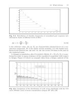
Fig. 2.4. Distribution of absolute frequencies of normalized gust responses into
subsequent classes of different levels of effect

Δσ =2·(
M
k
W
+
N
k
A
) (2.18)
is the reference value, M
k
an N
k
are characteristic internal forces of a con-
struction component, W is the elastic section modulus, A is the loaded area.
Stress levels between 0.9 ·Δσ and 1.0 ·Δσ can occure 2.9 times in 50 years in
the statistical mean.
A damage accumulation after Palmgren-Miner D =

i
(N
i
/N
ci
)isper-
formed in order to assess resistance of the considered component with respect
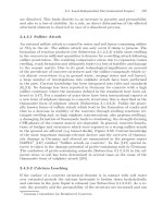
to fatigue. Figure 2.5 shows an example taken from a fatigue analysis of the
S - N c u r v e ( W ö h l e r c u r v e ) o f
s t r e s s c o n c e n t r a t i o n c a t e g o r y 3 6 *
Fig. 2.5. Comparison of the distribution of cyclic stress amplitudes with the S-N

curve (W¨ohler curve) of stress concentration category 36* after [30]
18 2 Damage-Oriented Actions and Environmental Impact
gust responses of steel archs of a road bridge. The considered cerb is suffi-
cient to resist the repeated gust impacts. The application of the Equations
2.12 or 2.17 permits a detailed and safe method for the fatigue analysis of
gust-induced effects at building structures.
2.1.2 Influence of Wind Direction on Cycles of Gust Responses
Authored by R¨udiger H¨offer and Hans-J¨urgen Niemann
Meteorological observations document that the intensity of a storm is
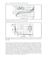
strongly related to its wind direction. Figure 2.6(a) shows the wind rosette of
the airport Hannover, Germany, as an example. The probability of the first
passage of the same threshold value can strongly vary for different sectors of
wind direction. That means that the risk of a high wind induced stressing of a
structural component is different between the wind directions. The failure risk
5m/s
15 m/s
25 m/s
35 m/s
90
◦
0
◦
270
◦
180
◦
5m/s
15 m/s
25 m/s
35 m/s

90
◦
0
◦
270
◦
180
◦
5m/s
15 m/s
25 m/s
35 m/s
90
◦
0
◦
270
◦
180
◦
90
◦
0
◦
270
◦
180
◦
0.25
0.50

0.75
1.00
(a) (b)
(c) (d)
Fig. 2.6. Rosettes of wind quantities at Hannover (12 sectors, 50 years return pe-
riod) (a) extremes of 10-minutes means of wind velocities at the airport of Hannover
at reference height of 10 m above ground (b) extremes of 10-minutes means of wind
velocities at a building location at building height of 35 m above ground (c) ex-
tremes of gust wind speeds at a building location at building height of 35 m above
ground (d) comparison of the load factors of the sectors; the largest load factor is
valid for the design of the fa¸cade element after Figure 2.8
2.1 Wind Actions 19
of the structure or structural components is determined by the superposition
of all probability fractions originating from the sectors of wind direction.
Usually, codes follow the conservative approach to assume the same prob-
ability of an extreme wind speed for all wind directions. In general, more re-
alistic and very often also more economic results can be achieved if the effect
of wind direction is considered. This can be done by employing wind speeds
for the structural loading which are adjusted in each sector with a directional
factor. Such procedure is in principle permitted by the Eurocode [32]. It is
left to the national application documents to regulate the procedures.
The wind load is a non-permanent load; within statical proofs of the load
bearing capacity it is employed using a characteristic value, which is defined
as a 98% fractile, and an associated safety factor of 1.5. A load level is required
which is exceeded not more than 0.02 times a year in a statistical sense. Such
value is statistically evaluated from the collective of yearly extremes of the
wind speeds. The intensity of the wind load is deduced from the level of the
wind speed, or more exact, from its dynamicpressure.Therelated statistical
parameters are used to determine the characteristic value of the load.
The wind load depends on the wind direction as the wind speed is differently

distributed regarding their compass, and as the aerodynamic coefficients varies
with respect to the angle of flow attack. Taking this into account the most
unfavourable load can originate from combining a lower characteristic value
of the wind speed, which might be associated to a directionalsector,andthe
related aerodynamic coefficient for this sector. In order to evaluate completely
the effect of the influence of the wind direction it is required to take the
structural response into account, e.g. after [227]. In such procedure a response
quantity, which is a representative value of the wind action, is evaluated with
the restriction to limit its exceedance probability of its yearly extremes to a
value lower than 0.02 instead of focussing on loads. Using this requirement the
characteristic wind velocities related to the different sectors can be deduced.
2.1.2.1 Wind Data in the Sectors of the Wind Rosette
The maximum wind load effect on a structural component is resulting from
the most unfavourable superposition of the function of the aerodynamic coeffi-
cient and the dynamic pressure. Both variables are independent and functions
of the direction of mean wind. The usual zoning in statistical meteorology into
twelve sectors of 30
◦
each is a sufficient resolution in order to include distri-
bution effects. The prediction of the risk requires an analysis of the extreme
wind velocities for each sector at the building location. If available a complete
set of data is taken from a local station for meteorological observations near
the considered building location. The wind statistics of a considered building
location in the city of Hannover in Germany is shown in Figure 2.6(a) as an
example. The wind rosette is evaluated from data collected at the observation
station at the airport of Hannover. The terrain in the environment of the sta-
tion is plain with a relatively homogeneous surface represented by a roughness
20 2 Damage-Oriented Actions and Environmental Impact
Table 2.1. Conversion of the wind data of the observation station at the airport of
Hannover into data for the building location

Sectors of wind directions
0
◦
30
◦
60
◦
90
◦
120
◦
150
◦
180
◦
210
◦
240
◦
270
◦
300
◦
330
◦
airport:
1 z
0
=0.05 m:
v

m
(z =10m)
in m/s
12.1 11.7 17.4 13.0 15.2 15.9 17.1 20.5 23.0 20.6 16.7 12.5
arena:
2 z
0
in m 0.44 0.27 0.31 0.24 0.24 0.08 0.10 0.11 0.36 0.36 0.36 0.35
3 k
r
· ln(
z
z
0
)
0.96 1.03 1.02 1.05 1.05 1.20 1.16 1.15 1.00 1.00 1.00 1.00
4 v
m
(z =35m) 11.7 12.1 17.7 13.7 16.0 19.0 19.9 23.7 22.9 20.5 16.6 12.5
5 I
u
(z =35m) 0.229 0.206 0.212 0.201 0.201 0.164 0.171 0.174 0.218 0.218 0.218 0.217
6 gust factor
v
v
m
1.540 1.494 1.506 1.485 1.485 1.409 1.423 1.429 1.520 1.520 1.520 1.518
7 v(z =35m) 18.0 18.1 26.7 20.3 23.7 26.8 28.3 33.8 34.8 31.2 25.3 19.0
of ca. z
0

=0.05 m in all of the sectors. The measurements have been conducted
in a standard height of 10 m above ground level, cf. J. Christoffer and M.
Ulbricht-Eissing [196]. N yearly extremes of the mean wind velocity v
m
are ranked in each sector F , and respective probability distributions are iden-
tified. In the presented example distributions of Gumbel-typewereadapted.
The occurrence probability of an extreme value in a year, which is lower than
a reference value v
m,ref
,iscalculatedfrom
P (v
m
≤ v
m,ref
)=F (v
m,ref
)=e
−e
−a(v
m,ref
−U)
(2.19)
In Equation 2.19 U is the modal parameter, and the parameter a describes the
diffusion. The wind velocities with return periods of 50 years for all sectors
are listed in Table 2.1, line 1. In opposite to the conditions at the observa-
tion station, the building location is surrounded by a terrain with strongly
non-homogeneous surface roughnesses. The effect of the varying roughnesses
superpose the undisturbed conditions evaluated for the location of the obser-
vation station.
These additional effects influence the wind velocity in reference height,

its profile and the profile of gustiness over height, which vary between the
directions according to the respective roughness conditions of a sector.
The surface roughnesses for each sector are required. The local roughness
lengths z
0
of the surface roughness is analysed from aerial photographs over
a radius of 50 to 100 times the height of the considered building, e.g. ca. 5 km
in case of the considered stadium, Figure 2.7. Mixed profiles are evaluated for
those sectors with significantly changing surface roughnesses; for approxima-
tion an equivalent roughness length is adapted. The results are shown in line 2
of Table 2.1; the conditions within each sector are described by conversion fac-
tors related to the undisturbed wind rosette. The factor in line 3 of Table 2.1
relates the mean wind speeds with a return period of 50 years at the building
2.1 Wind Actions 21
0°
b
90°
b/5
c =-1.4
p
Fig. 2.7. Roughness lengths of the ter-
rain in the farther vicinity of the building
location [771]
Fig. 2.8. Sketch of a building contour
(top view) with b<2 h and fa¸cade el-
ement exposed to a pressure coefficient
c
p
= −1.4 [32] at the eastern fa¸cade in
thecaseofwindsfrom0

◦
location at a building height of 35 m of the stadium and the reference wind
speed of the same return period at the location of the observation station in
reference height of 10 m. The logarithmic law for the profile of the mean wind
velocities is applied (Equation 2.20). The terrain factor k
r
is evaluated using
an empirical relation (Equation 2.21).
v
m
(z,z
0
)
v
m
(z
ref
,z
0ref
)
= k
r
· ln(
z
z
0
) (2.20)
k
r
=(

z
0
z
0ref
)
0,07
·
1
ln(z
ref
/z
0ref
)
(2.21)
The wind velocities at the building location with a return period of 50 years
are evaluated for each sector and are listed in line 4 of Table 2.1.
As shown before, mean and gust wind speeds and the respective dynamic
pressures are applied to determine equivalent loads which represent the result-
ing wind loading for design procedures. The dynamic gust pressure is calculated
from the mean dynamic pressure q
m
and the turbulence intensity I
u
.
q =(1+2g · I
u
·Q
0
) · q
m

(2.22)
The gust velocity in the last row of Table 2.1 is calculated from Equation 2.23,
where g is the peak factor and Q
0
is the quasi-static gust reaction. Q
2
0
is also
called background response factor after [32].
22 2 Damage-Oriented Actions and Environmental Impact
v =

1+2gQ
0
I
u
· v
m
(2.23)
For simplicity Q
0
can consistently be determined from 2 gQ
0
= 6 assigning to
Q
0
its maximum value 1. It has to be pointed out that the surface roughness
is also affecting the turbulence intensity, as shown in line 5 of Table 2.1.
The statistical evaluation for all sectors leads to a mean wind of 50 years
return period of 23.8m/s at the building location.

Figure 2.6(b) represents the rosette of mean wind speeds at the building
location. In comparison of both wind rosettes, representing the building lo-
cation and the location of the observation station, it can be concluded that
the main character of the local wind climate is preserved but relevant changes
due to the terrain roughness are introduced.
2.1.2.2 Structural Safety Considering the Occurrence Probability
of the Wind Loading
The wind load effect on a structure can be expressed in terms of a response
quantity Y . For a linear, stiff structure without dynamic amplification, Y is
calculated from:
Y (Φ)=
1
2
ρv
2
Φ
·

A
η
p
(r) · c
p
(r, Φ) · dA (2.24)
in which: η
p
influence factor for the pressure p acting at the point on the
surface of the structure; r - local vector; c
p
pressure coefficient at a point of

the surface of the structure for a given wind direction Φ; ρ - mass density of
air; A - pressure exposed influence area.
A certain response force Y forms the basis for the determination of a char-
acteristic wind velocity v
ik
, which is valid over the sector with the central
wind direction Φ
i
. The starting point is v
i,lim
:
Y
i,lim
(Φ
i
)=C
Y
(Φ
i
) ·
1
2
ρ ·v
2
i,lim
(2.25)
In Equation 2.25 the response Y
i,lim
is determined as an equivalent wind
effect by use of the gust velocity v. The wind effect admittance depending on

the wind direction Φ, C
Y
= C
Y
(Φ), is identical to the integral in Equation
2.24. It covers the distribution and the value of the aerodynamic coefficient
within the influence area of the load as well as the mechanical admittance,
which is the transfer from the dynamic pressure into the response quantity.
This operation is conducted for a selected wind direction Φ
i
. In a second step
the complete risk is evaluated as the exceedance probability of the response
quantity Y , which adds up from the contributions from each sector. The safety
requirements are met if the total risk has a value smaller than 0.02.
In case of a risk larger 0.02 an increased value of the v
i,lim
enters into the
iteration until a value smaller 0.02 is achieved. In an analogeous manner a
2.1 Wind Actions 23
decreased value of v
i,lim
is introduced aiming on an economical optimization
if the first iteration yields a value much smaller than 0.02.
The total risk of exceeding the bearable response quantity Y
i,lim
,oras
complementary formulation, the probability of non-exceedance of Y
i,lim
,is
proved within the following steps. The main idea of the procedure is to make

use of combinations C
Y
(Φ) ·
1
2
ρ · v
2
Φ,lim
instead of a global C
Y
·
1
2
ρ · v
2
.A
probability of non-exceedance of 0.98 of the applied force must be guaranteed
forbothinthesectorsandintotal.
C
Y
(Φ
i
) ·
1
2
ρ ·v
2
i,lim
= C
Y

(Φ) ·
1
2
ρ ·v
2
Φ,lim
(2.26)
The velocity limit v
Φ,lim
for a sector Φ results as
v
Φ,lim
=

C
Y
(Φ
i
)
C
Y
(Φ)
·v
i,lim
=

1
a(Φ)
· v
i,lim

(2.27)
The effect of the direction of the wind on the wind effect is expressed through
a directional wind effect factor:
a(Φ)=
C
Y
(Φ)
C
Y
(Φ
i
)
(2.28)
The probability P (v ≤ v
Φ,lim
)=F
Φ
(v
Φ,lim
) of the non-exceedance of v
Φ,lim
within the sector Φ also applies for the response Y ≤ Y
i,lim
. F (v
Φ,lim
)can
be calculated from the probability distribution of the mean wind velocity in
the sector as given by Equation 2.19. The probability of the non-exceedance
of the limit Y
i,lim

after Equation 2.25 under the condition of a certain v
i,lim
in sector Φ
i
is satisfied from a product (Equation 2.29) of all non-exceedance
probabilities under the condition that the yearly extremes in the different
sectors are statistically independent.
P (Y ≤ Y
i,lim
)=P ((v ≤ v
1,lim
)

(v ≤ v
2,lim
)

···

(v ≤ v
12,lim
))
=

12
1
F
Φ
(v
Φ,lim

) ≥ 0.98
(2.29)
The considered value of the gust speed is adequate if the exceedance probabil-
ity P (Y>Y
i,lim
) is less or equal 0.02 which corresponds to the probability of
non-exceedance of (1 − 0.02) = 0.98, Equation 2.29. Obviously, the condition
P (Y = Y
i,lim
) ≥ 0.98 must be observed in any sector.
2.1.2.3 Advanced Directional Factors
The responses of a structure must be taken into consideration for the deter-
mination of the relevant wind speeds and wind loads for each sector. This
24 2 Damage-Oriented Actions and Environmental Impact
Table 2.2. Determination of a reduced characteristic suction force on the fa¸cade
element after Figure 2.8 through the consideration of the effect of wind direction
on loading. line 1: extreme gust speed at a building location at Hannover at build-
ing height of 35 m; line 2: c
p,10
-values at the considered fa¸cade element for wind
flow from the respective directions; line 3: directional wind effect factor after Equa-
tion 2.8; line 4: iterative determination of applicable wind speeds in sectors and
associated non-exceedance probabilities in sectors; line 5: applicable fraction of
codified standard load after the proposed method
Sectors of wind directions
0
◦
30
◦
60

◦
90
◦
120
◦
150
◦
180
◦
210
◦
240
◦
270
◦
300
◦
330
◦
1 18.0 18.1 26.7 20.3 23.7 26.8 28.3 33.8 34.8 31.2 25.3 19.0
2 -1.4 -1.4 – – – -0.8 -0.8 -0.8 -0.6 -0.6 -0.6 -1.4
3 1 1 0 0 0 0.57 0.57 0.57 0.36 0.36 0.36 1
4 18.0 18.1 ∞ ∞ ∞ 35.5 37.5 44.8 58.0 52.0 42.2 19.0
0.98 0.98 1.0 1.0 1.0 0.98 0.98 0.98 0.98 0.98 0.98 0.98
18.2 18.3 ∞ ∞ ∞ 36.0 38.1 45.5 59.0 52.8 42.9 19.2
0.9985 0.9985 1.0 1.0 1.0 0.9985 0.9985 0.9985 0.9985 0.9985 0.9985 0.9985
5
0.194 0.196 – – – 0.434 0.486 0.694
0.874
0.701 0.462 0.216

can be achieved using the values of the wind effect admittance C
Y
(Φ)forthe
respective sectors.
The procedure of calculating the characteristic wind speed in the sectors is
exemplified in Table 2.2 for a building located at Hannover, Germany. The fix-
ing forces of fa¸cade claddings due to suction is considered. Figure 2.6 shows
a topview sketch of a building cubus of 35 m height with fa¸cades oriented in
northern, eastern, southern and western directions. The question is if reduced
values of the suction forces at the cladding elements at the edge of the eastern
fa¸cade can be adopted as the wind rosettes clearly indicate different wind ex-
tremes when comparing the sectors, cf. line 1 in Table 2.2. Wind from eastern
directions generate pressure forces at the element, whereas suction forces at the
same element are generated through winds from all other sectors. Suction co-
efficients from [26], Table 3, are used to describe the aerodynamic admittance
in simplified terms. An element size of more than 10 m
2
is assumed. The pres-
sure minimum — or maximum suction — occurs for northern directions and is
described through the pressure coefficient c
p
= −1.4forh/b ≥ 5, h =35m.
Southern wind directions generate a coefficient of c
p
= −0.8, c
p
= − 0.6isin-
serted for western wind directions (cf. line 2 in Table 2.2).
The directional wind effect factor a(φ) in line 3 after Equation 2.28 is
calculated refering the sectorial pressure coefficents to the minimum pressure

coefficient c
p
= c
p,min
= −1.4. The results of two iterations are listed in
line 4. The first two rows represent v
Φ,lim
= v
i,lim
and the corresponding
probability of non-exceedance F
Φ,lim
(v
Φ,lim
) which remains 0.98 according to
the probability of non-exceedance of the values given in line 1, or it is 1 in
sectors 0
◦
,60
◦
and 90
◦
as only pressure instead of suction can occur here. The
application of Equation 2.29 leads to P =0.8171 < 0.98. In a second iteration
the extreme wind speeds are increased in such a way that the total probability
2.1 Wind Actions 25
of non-exceedance after Equation 2.29 results to be larger or equal to 0.98.
The third and fourth row in line 4 of Table 2.2 represent a valid solution for
which P =0.9866 and results larger than the required value of P =0.98.
The codified standard design procedure requires a reference wind speed of

v
ref
=25m/s irrespective the wind direction. The calculation of a gust speed
after the wind profile for midlands ([26], Table B.3) leads to a characteristic
gust speed of v =41.3m/s at building height of 35 m. The standard suction
force for the considered element — without any consideration of the influ-
ence of wind directions — must be calculated as Y =
1
2
ρ · v
2
· c
p
· A.The
applicable characteristic suction force after Equation 2.25 — with consider-
ation of the influence of wind directions — can be calculated as a fraction
(c
p
(φ) · v
2
φ,lim
)/(c
p,min
· v
2
ref
) of the standardized characteristic value. The
quotient is listed in line 5 of Table 2.2, and it is represented in Figure 2.6,
(d). The largest factor in line 5 must be applied. The respective characteris-
tic velocity is ca. 59 m/s but the associated characteristic suction force after

Equation 2.26 is lower than the standard suction force after the code. The
reason is in the application of the much higher pressure coefficent — or lower
suction coefficient — of c
p
= −0.5 for wind in the sector 240
◦
instead of
c
p
= −1.4.
The procedure can also be adopted for a fatigue analysis after Equation 2.9.
2.1.3 Vortex Excitation Including Lock-In
Authored by J¨org Sahlmen and M´ozes G´alffy
Vortex excitations represent an aerodynamic load type which can cause
vibrations leading to fatigue, especially for slender bluff cylindrical structures
— bridge hangers, towers or chimneys.
The nature of air flow around the structure depends strongly on the wind
velocity and on the dimensions of the structure. Accordingly, different wind
velocity ranges can be defined, depending on the value of a non-dimensional
parameter called the Reynolds-number
Re =
¯uD
ν
. (2.30)
Here, ¯u represents the mean wind velocity, D is the significant dimension of the
body in the across-wind direction — for cylindrical structures, the diameter
—andν =1.5 ·10
−5
m
2

/sisthekinematicviscosityofair.
In the Reynolds-number range between 30 and ca. 3 · 10
5
, vortices are
formed and alternately shed in the wake of the cylinder creating the von
K
´
arm
´
an vortex trail (Figure 2.9) and giving rise to the lift force — an alter-
nating force which acts on the structure in the across-wind direction.
The nature of the vortex shedding and of the lift force is considerably
influenced by the wind turbulence
I
u
=
σ
u
¯u
, (2.31)
26 2 Damage-Oriented Actions and Environmental Impact
Fig. 2.9. Von K
´
arm
´
an vortex trail formed by vortex shedding
where σ
u
denotes the standard deviation of the stochastically fluctuating wind
velocity u. In a smooth wind flow, i. e. if the wind turbulence is low (I

u
≤ 0.03),
the across-wind force is a harmonic function of the time t:
F
l
(t)=
ρ¯u
2
2
DC
l
sin 2πf
s
t. (2.32)
Here, F
l
denotes the lift force per unit span, ρ =1.25 kg/m
3
is the density of
air, C
l
is the dimensionless lift coefficient and
f
s
= S
¯u
D
(2.33)
is the frequency of the vortex shedding, also called the Strouhal-frequency.
The non-dimensional coefficient S in (2.33) is the Strouhal-number which

depends on the shape of the structure; its value for cylinders is S ≈ 0.2. In a
turbulent flow, the excitation frequencies are distributed in an interval around
the mean frequency, the width of the interval depending on the turbulence.
When the Strouhal-frequency approaches one of the natural frequencies
f
n
of the structure
1
and the structure begins to oscillate at higher ampli-
tudes because the resonance, an aeroelastic phenomenon, the so-called lock-in
effect occurs. This results in the synchronization of the vortex shedding pro-
cess to the motion of the excited structure (Figure 2.10), acting as a negative
aerodynamic damping, and can lead to very large oscillation amplitudes. Con-
sequently, the lock-in effect can play an essential role in the evolution of the
fatigue processes in the damage-sensitive parts of the structure.
The width of the lock-in range is zero for a fixed system and increases
with increasing oscillation amplitude. As the amplitude depends on mass and
damping, these system-parameters have a large influence on the lock-in effect.
This influence can be numerically catched by introducing the dimensionless
Scruton-number
Sc =
2μδ
ρD
2
, (2.34)
where μ denotes the mass of the structure per unit length, and δ is the
structural logarithmic damping decrement. The width of the lock-in range is
1
Generally only the first natural frequency is of practical importance.
2.1 Wind Actions 27

Fig. 2.10. Dependence of the vortex shedding frequency f
v
on the wind velocity ¯u.
f
n
is the natural frequency of the structure
reduced with increasing Scruton-number, and for very large values of Sc,no
lock-in effect occurs at all.
In the case of a uniform smooth flow, the lift force per unit span acting on
a circular cylinder fixed in both the along-wind and across-wind directions is
given by (2.32). However, the force is not fully correlated along the cylinder
span. If the cylinder is allowed to oscillate, the magnitude of the lift force and
also the correlation increases. The equation of motion of the cylinder is given
by
m¨y + c ˙y + ky = F
l
(u, D, y, ˙y, ¨y,t), (2.35)
where y denotes the across-wind displacement, m, c and k are the mass, the
damping coefficient and the stiffness of the cylinder per unit span. As the lift
force per unit span F
l
depends not only on the wind velocity, on the cylinder
diameter and on time, but also on the displacement, on the velocity and on the
acceleration of the structure
2
, it is not a trivial task to establish its explicite
expression. Furthermore, the wind velocity u(t) is a stochastic variable which
generally describes a turbulent wind process, and consequently a suitable wind
load model must also correctly describe the oscillations in turbulent flow.
Much effort has been done in order to find an expression for the across-wind

force which fits the experimentally observed facts. However, all of the wind-
load models developed up to the present can only describe the experimentally
observed oscillations correctly if some limiting conditions are fulfilled.
2.1.3.1 Relevant Wind Load Models
The Ruscheweyh-model [695], which is implemented in the German Codes
DIN 4131 (Steel radio towers and masts) and DIN 4133 (Steel stacks), de-
scribes the across-wind oscillations in the time domain. The lift force per unit
2
The lift force also depends on the roughness of the cylinder surface, which is here
not explicitely shown.
28 2 Damage-Oriented Actions and Environmental Impact
span is given by (2.32). The lift coefficient is C
l
=0.7forRe ≤ 3 × 10
5
,
for higher Reynolds-numbers, C
l
decreases. It is assumed that the lift force
acts over the correlation length L
c
, which is the length-scale of the synchro-
nized vortex shedding along the cylinder span. The increase of correlation
with increasing oscillation amplitude A
y
is described by the function
L
c
=
⎧

⎪
⎨
⎪
⎩
6D for A
y
≤ 0.1D
4.8D +12A
y
for 0.1D<A
y
< 0.6D
12D for A
y
≥ 0.6D
(2.36)
The width of the lock-in range is set to ±15 % around the critical velocity
u
c
=
Df
n
S
, (2.37)
which leads to a Strouhal-frequency equal to the natural frequency: f
s
= f
n
.
This model predicts the oscillation amplitudes of slender cylindrical struc-

tures in a smooth wind flow for constant mean wind velocities within and
outside of the lock-in range with a remarkable accuracy. Large estimation
errors occur, however, in the case of high turbulence, or if the mean wind
velocity considerably varies in time — especially in the case of entering or
exiting the lock-in range.
The Vickery-model [811] uses a frequency-domain-approach to describe
the across-wind vibrations. Assuming a Gaussian distribution for the spectral
density of the lift force, the standard deviation (rms-value or effective value)
of the across-wind deflection is obtained as
σ
y
=
C
Lσ
ρD
3
8π
2
S
2
m
e

√
πL
c
h
2Bξ
f
3

s
f
3
n
e
−
(
1−f
n
/f
s
B
)
2
. (2.38)
Here, C
Lσ
is the lift coefficient expressed as rms-value, m
e
and ξ are the
effective mass and damping ratio of the structure, h is the height of the cylin-
der and B is a dimensionless parameter which describes the relative width
of the Gaussian spectral peak of the lift force. The parameters C
Lσ
≈ 0.1,
L
c
≈ 0.6 D and B are obtained from fits to experimental data; obviously, B
depends on the wind turbulence.
The model is suitable for predicting the oscillation amplitudes, both in

smooth and turbulent flow, but it is limited to the case of stationary flow, i. e.
to constant mean wind velocities, and it doesn’t take the lock-in effect into
consideration.
The model of Vickery and Basu [810] describes the across-wind oscilla-
tions in smooth or turbulent flow, with mean wind velocities outside or within
the lock-in range. The lift force is written as the sum of two forces: a narrow-
band stochastic term with a normal distribution of the spectral density and a
motion dependent term — negative aerodynamic damping — which describes
the lock-in effect. For the lock-in range, the rms-value of the displacement is
obtained as
2.1 Wind Actions 29
σ
y
=2.5
C
l
ρD
3
L
c
16π
2
S
2

π
m
e
(μ
e

ξ + μξ
a
)

h
0
ψ
2
(z) dz
, (2.39)
where μ and μ
e
are mass and effective mass of the structure per unit span,
ψ(z) is the value of the normalized mode shape at height z,andξ
a
is the
aerodynamic damping ratio. The aerodynamic damping is negative in the
lock-in range, and it depends on the ratio ¯u/u
c
, on the turbulence and on the
Reynolds-number. Additionally, a dependence on the oscillation amplitude
is defined in such a way that it limits the amplitude to a predefined value.
The most exhaustive model of vortex-induced across-wind vibrations has
been developed by ESDU [262], mainly based on the work of Vickery and
Basu [810]. The response equations give the standard deviation of the oscilla-
tion amplitude and incorporate the influences of turbulence and of the lock-in
effect. The system response is obtained from the superposition of a broad-
and of a narrow-band term. A very large variety of parameters, such as the
surface roughness or the integral length of the turbulent wind, is included in
the calculation. Also, the dependence of the lock-in range width on the oscil-

lation amplitude is taken into consideration. Because of their complexity, the
response equations will not be presented here. Like all the models presented
above, also this model is only suitable to describe the across-wind vibrations
in a stationary or quasi-stationary flow, i. e. if the mean wind velocity doesn’t
change too rapidly and if there is no transition into or from the lock-in range.
Based on the normal distribution of the lift force spectral density S
F
,sug-
gested by Vickery and Clark [811], Lou has developed a convolution model
[507] which describes the lift force in the time-domain, for a stationary tur-
bulent flow, outside of the lock-in range:
F
l
(t)=
ρ
2
DC
l

t
0
βu
2
(τ) e
−
¯
ξ ¯ω(t−τ )
cos ¯ω(t − τ) dτ, (2.40)
¯ω =2πS¯u/D denoting the Strouhal circular frequency corresponding to
themeanwindvelocity¯u. From the assumption of the normal distribution

for S
F
, the parameters β and
¯
ξ can be determined as
β =¯u

√
2π ln 2 I
u
¯ω(2 + 2 ln 2 I
2
u
)
S
u
(¯ω)(1 + 2 ln 2 I
2
u
)
,
¯
ξ =
√
ln 4 I
u
, (2.41)
where S
u
is the spectral density of the wind velocity.

2.1.3.2 Wind Load Model for the Fatigue Analysis of Bridge
Hangers
In the project C5 of the Collaborative Research Center (SFB) 398, the vortex-
induced across-wind vibrations of the vertical tie rods of an arched steel bridge
in M¨unster-Hiltrup have been analysed for the purpose of a fatigue analysis of
30 2 Damage-Oriented Actions and Environmental Impact
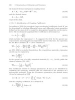
Fig. 2.11. Wind velocity, measured and simulated deflection vs. time for the bridge
hanger 1 (left) and 2 (right). The horizontal lines in the upper panels show the mean
width of the lock-in range
their extremely damage-sensitive welded connections. Therefor, the vibrations
of two hangers have been filmed by digital cameras, and the time histories
of the deflections have been extracted from the videos by means of a Java
program. Simultaneously, the fluctuating wind velocity has been recorded with
an ultrasonic 3D-anemometer. The mean wind velocity varied with time in
such a way, that one of the hangers entered and exited the lock-in range several
times during the measurement, while the other one stayed outside of the lock-
in range, see Figure 2.11. Because of the low oscillation amplitude, the lock-in
range of the second hanger was very narrow; it lies within the width of the
horizontal line in the upper right panel.
In order to check the validity of the previously presented wind load mod-
els for bridge hangers, the amplitudes measured on hanger 1 in the lock-in
range, in the time-interval between 8.5–12.5 min have been compared to the
predictions of the Ruscheweyh- [695] and ESDU-models [262]. The experi-
ment shows a peak amplitude of ca. 9 mm and an rms-amplitude of ca. 6 mm,
while the Ruscheweyh-model predicts peak amplitude of about 5 mm and
the ESDU-model an rms-amplitude of ca. 30 mm.
As both models show a substantial discrepancy compared to the mea-
sured values, a new wind load model for the across-wind vibrations of bridge
tie-rods in non-stationary, turbulent flow, including the lock-in effect, has
been developed [296], based on the model by Lou [507]. For this purpose, a

2.1 Wind Actions 31
power-function dependence of the parameter β in (2.40) on the fluctuating
wind velocity u has been supposed:
β = Ku
n−2
, (2.42)
with the fit-parameters K and n. Furthermore, in order to describe the non-
stationary wind process, the mean values in (2.40) have been replaced by
the corresponding time-dependent quantities; only the wind turbulence I
u
is
supposed to be constant. The lift force per unit span obtained this way is:
F
l
(t)=
ρ
2
DC
l
K

t
0
u
n
(τ) e
α(t,τ)
cos ϕ(t, τ)dτ, (2.43)
with
α(t, τ)=

√
ln 4 I
u

τ
t
ω(θ) dθ, ϕ(t, τ)=

τ
t
ω(θ) dθ + ϕ
0
(t). (2.44)
ω(θ)=2πSu(θ)/D is the Strouhal circular frequency corresponding to the
fluctuating wind velocity u at the time moment θ. It is supposed that the
lift force acts over the correlation length L
c
which can be determined from
equation (2.36).
The phase angle ϕ
0
in (2.44) describes the lock-in effect. For wind velocities
in the lock-in range, it is set in phase with the rod motion:
ϕ
0
(t)=π +arctan
˙y(t)
ω
n
y(t)

, (2.45)
outside of the lock-in range, it is set to 0. ω
n
=2πf
n
denotes the angular
natural frequency of the rod. The increase of the force amplitude caused by the
phase-synchronization is compensated by the reduction of the multiplicative
parameter K in equation (2.43) for the lock in range.
It has been assumed that the lock-in range is symmetric with respect to the
critical wind velocity (2.37) with a half width Δu depending on the oscillation
amplitude A
y
according to a simple parabolic function (Figure 2.12). The
parabola is defined by three points, P
1
,P
2
and P
3
, obtained from fits to the
experimental data.
The fit of the model parameters to the experimental data has been per-
formed by simulating the vortex-induced vibrations in the time domain, on
a finite-element model of the hanger, which has been excited by the force
calculated using equation (2.43) applied to the experimental wind data u(τ).
The time dependent deflections have been calculated using the Newmark-
Wilson time-step method, applying C
l
=0.5andL

c
=6D. The time histo-
ries obtained for the fitted values of the model parameters, K = 175m
−1
and
n = 3, are shown in the lower panels of Figure 2.11. For the lock-in range, the
multiplicative parameter K has been reduced by a factor 4.
32 2 Damage-Oriented Actions and Environmental Impact
Fig. 2.12. Width of the lock-in range for bridge tie rods
The time history of the measured and simulated oscillation amplitudes
shows a remarkable similarity for both hangers (Figure 2.11). Furthermore,
the averaged rms-amplitudes of the simulated deflections are very close to the
values determined from the experiment: for hanger 1, 3.81 mm is obtained for
both the measured and simulated data, while for hanger 2, measurement and
simulation yield 0.133 mm and 0.130 mm respectively.
The wind load model has also been validated by wind tunnel measure-
ments,carriedoutonarigidcylinder,elasticallysuspendedinsuchaway
that it could oscillate only in the across-wind direction. Wind velocity and
displacement have been simultaneously recorded for 17 fixed values of the
mean wind velocity. The displacements of both ends have been averaged in
order to eliminate the rotational vibration of the cylinder around the axis
parallel to the wind direction. The fit of the model parameters has been per-
formed analogously to the full scale case, applying the same values for the
parameters C
l
and L
c
, obtaining K =23m
−1
and n =3.Thevaluesfor

the full scale and the wind tunnel experiments differ because K obviously
depends on the wind turbulence (see eq. (2.41) and (2.42)). Again, for the
lock-in range, the parameter K has been reduced by the factor 4.
The measured and simulated time histories of the amplitudes are shown
in Figure 2.13 for a representative measurement within and another outside
of the lock-in range. In both cases, the measured and the simulated data
show time-dependent amplitudes with qualitatively and quantitatively similar
characteristics. The ratio of the simulated to measured rms-amplitudes of the
displacement varies between 0.47 and 1.95 for the different fixed mean wind
velocities, which can be considered as a good agreement between model and
experiment, in comparison to other models: The amplitudes are overestimated
by a factor of ca. 7 by the Ruscheweyh- and by a factor of ca. 11 by the
ESDU-model.
2.1 Wind Actions 33
Fig. 2.13. Measured and simulated amplitude of the displacement within and out-
side of the lock-in range
2.1.4 Micro and Macro Time Domain
Authored by M´ozes G´alffy and Andr´es Wellmann Jelic
In modeling stochastic, especially time-variant fatigue processes, commonly
the time scale is split into a micro and a macro time domain. In the micro
time domain, loading events and resulting fatigue events are simulated. The-
oretically, the loading and fatigue process can be considered as continuous in
the micro time domain, but for practical calculations discrete realizations of
these processes are used, which are separated in time by a constant increment
called time step. The macro time domain is used for estimating the lifetime
of the structure, taking into consideration the succession of fatigue events in
time. The splitting procedure is applicable to any stochastic loading which
causes fatigue — e. g. wind, traffic, sea-waves, etc.
The reasons for splitting the time scale are:
• Within the micro time domain, the system properties, and in most cases

also the excitation process, can be considered time-independent. Conse-
quently, the simulation of a fatigue process in this time domain — a fatigue
event — can be performed using time-independent stiffness, damping and
34 2 Damage-Oriented Actions and Environmental Impact
Fig. 2.14. Sample realizations of a renewal process (left) and of a pulse-process
(right)
massmatricesandanexcitationforcederivedfromastationaryrandom
function (generally white noise).
• The numerical simulation of the fatigue process over the macro time do-
main would result in unacceptably large computation times, especially for
complex structures, where the solution of the equation of motion implies
a laborious finite-element calculation at every time-step.
The advantage of the time scale splitting is that the fatigue results obtained for
a load event in the micro time domain (e. g. using the rainflow cycle counting
method) can be used in the macro time domain several times, without the need
of recalculating the time histories of the loads and of the system responses.
Generally, the length of the micro time domain is chosen btw. 1 ms and
1 s, depending on the properties of the structure and the loading. For some
applications, however, considerably larger durations are needed, e. g. for the
lifetime analysis of bridge hangers, performed in the project C5 of the Col-
laborative Research Center (SFB) 398. Because of the large mass and small
damping of the tie rods (logarithmic damping decrement δ ≈ 6 × 10
−4
), the
system answer to changes in the nature of the excitation force (e. g. on entering
or exiting the lock-in range, see Section 2.1.3) is very slow and consequently it
was necessary to choose a duration of ca. 1.5 hours for the micro time domain.
Another uncommon feature of this application is that because of the lock-in
effect, the stochastic excitation force cannot be considered stationary, even in
the micro time domain [295].

The macro time domain spans the whole lifetime of the structure, implying
an order of magnitude of several years.
2.1.4.1 Renewal Processes and Pulse Processes
In the macro time domain, the succession of the fatigue events is numerically
represented by discrete processes which occur at certain moments of time
2.2 Thermal Actions 35
t
i
, called renewal points. Each process causes a jump in the fatigue function,
between the renewal points the function remains constant. The processes with
constant height are called renewal processes, and those with variable height
are called pulse processes. Renewal processes can be characterized by one
single stochastic variable representing the length of the renewal period (the
period between two successive renewal points). For pulse processes, a second
stochastic variable is needed for the full description: the pulse height.
Figure 2.14 presents the time dependence of the state function (e. g. fatigue)
for a renewal process, represented by the number N of the occured processes,
and of a pulse process, characterized by the pulse height X.
2.2 Thermal Actions
Authored by J¨org Sahlmen and Anne Spr¨unken
Climatic conditions (e.g. air temperature, solar radiation, wind velocity)
cause a non-linear temperature profile within a structure or a structural com-
ponent and stress due to thermal actions is induced. For the design and life-
time analysis of many engineering structures (e.g. bridges, cooling towers, tall
buildings, etc.) thermal effects, in combination with moisture and chemical
actions, remain an important issue.
2.2.1 General Comments
Authored by J¨org Sahlmen and Anne Spr¨unken
Temperature changes generate expansions or contractions, hence consider-
able stress may occur. The amount of stress is depending on the magnitude of

loading. In the elastic range of deformation the material returns to its original
dimension or shape when the load is removed. When subjected to sustained
or long-term loading, many building materials experience additional defor-
mation, which does not fully disappear when the loading is removed. Due
to this special load cracks may occur and deterioration starts or proceeds.
As a consequence the deterioration over time leads to a reduction of stiffness
of the structure. The implementation of affected non-linearities due to ther-
mal loads in the design process and lifetime analysis is still part of ongoing
research. The numerical modelling of the temperature effects on structures
based on experimental results are in the focus of this chapter.
2.2.2 Thermal Impacts on Structures
Authored by J¨org Sahlmen and Anne Spr¨unken
Permanent change of meteorological conditions (e.g. cloudiness, rain, sunny
periods, etc.) leads to non-stationary und locale site-dominated loads on a
structure. For the optimization of lifetime analysis a numerical algorithm is
36 2 Damage-Oriented Actions and Environmental Impact
needed to describe the physical thermal load scenario on an observed structure
or structural component. A realistic temperature field, based on experimental
data, has to be modelled to simulate the thermal transmission and moisture
flux within a material with the final aim to determine the time dependent
stress acting. Parameters like heat transfer and heat storage as well as the
content of moisture have to be considered [517, 74, 704, 463]. Further more
material and site conditions of the observed structure (location, climate, ori-
entation, surrounding properties, etc.) have to be implemented in a numerical
optimization model of thermal actions [518].
The process of heat transmission in materials is elementary controlled by
three phenomena [807]:
• heat conduction
• natural convection
• thermal radiation

In the following the physical fundamentals of heat transmission are briefly
described.
Material properties and structure dimensions are affecting directly the heat
conduction and the storage capacity. The rate at which heat is conducted
through a material is proportional to the area normal to the heat flow and
the temperature gradient along the heat flow path. For a one dimensional,
steady-state heat flow the rate is expressed by Fourier’s differential equation:
Q = −λdT/dh = −λgradT (2.46)
with: T = T (x = h) − T (x = 0) and assuming stationary heat transfer the
formula rearranges to:
Q = −λA(δT/h) (2.47)
where:
λ = thermal conductivity [W/mK]
Q = rate of heat flow [W]
δT = temperature difference [K]
A=contactarea[m
2
]
h = thickness layer [m]
Thermal conductivity λ is an intrinsic property of a homogeneous material
which describes the material ability to conduct heat. This property is indepen-
dent of material size, shape or orientation. For non-homogeneous materials,
those having glass mesh or polymer film reinforcement, the term relative ther-
mal conductivity is used because the thermal conductivity of these materials
depends on the relative thickness of the layers and their orientation with re-
spect to the heat flow direction.
The thermal resistance R is another material property which describes the
measure of how a material of a specific thickness resists to the flow of heat.
This parameter is defined as follows:
2.2 Thermal Actions 37

R = A(δT/Q) (2.48)
Hence, the relationship between λ and R is shown by the substitution of 2.47
and 2.48 and rearranging to the form:
λ = h/R (2.49)
Equation 2.49 reflects that for homogeneous materials, thermal resistance is
directly proportional to the thickness. For non-homogeneous materials, the
resistance generally increases with thickness but the relationship is maybe
non-linear.
Following this relation Eurocode 1 [19] is using a concept for the determi-
nation of the total resistance value as follows:
R
tot
= R
in
+

(h
i
/λ
i
)+R
out
(2.50)
where:
R
in
= thermal resistance at inner surface [m
2
K/W]
R

out
= thermal resistance at outer surface [m
2
K/W]
λ
i
= thermal conductivity of layer i [W/mK]
h
i
= thickness of layer i [W/mK]
The process of convection is dominated by the climatic conditions like wind,
temperature, humidity, etc. Convection describes the transfer of heat energy
by circulation and diffusion of the heated material. The fluid motion of the
surrounding air is caused only by buoyancy forces set up by the temperature
differences between the outer surface of the structure and the air temperature.
The basic equation for the convective heat transfer is given as follows:
Q
conv
= α
conv
(T
air
− T
surface
) (2.51)
where:
α
conv
= convection heat transfer coefficient [W/m
2

K]
T
air
=airtemperature[K]
T
surface
= surface temperature of the structure [K]
Thermal radiation, essentially induced by the visible and non-visible light
of the sun, consists of electromagnetic waves with different wavelengths (see
Figure 2.15). The energy which a wave is able to transport is related to its
wavelength. Shorter wavelengths carry more energy than longer wavelengths.
The transported energy is released when these waves are absorbed by an
object or structure.
Due to solar radiation thermal actions on structures could be subdivided
into two general types of solar impact depending on the wavelength:
• Short wave radiation with the highest heat energy content is described as
global radiation. It includes the direct and the diffuse part of the thermal
action on a structure as well as the reflected solar radiation from the
immediate vicinity (see Figure 2.16) of the observed object.
38 2 Damage-Oriented Actions and Environmental Impact
Fig. 2.15. Wavelength of the visible light
diffuse
direct
atmospheric
anti-radiation
reflection
wind
air-temperature
reflection of
atmospheric

anti-radiation
radiation of
immediate
vicinity
reflection of
global solar
radiation
Fig. 2.16. Climatic load on a structure
• Long wave radiation contains the atmospheric anti-radiation with its re-
flection to the surrounding area and to the atmosphere.
Additionally to the described external actions, the reflection of radiation at
the structure is influencing the thermal stress. Figure 2.16 shows all types of
radiation having a part on the thermal impact of a structure [517, 74, 286].
Heat transfer due to solar radiation is expressed by Boltzmann’s equation
as follows:
Q
rad
= α
rad
(T
emitter
− T
absorber
) (2.52)
2.2 Thermal Actions 39
where:
α
rad
= heat transfer coefficient due to radiation [W/m
2

K]
T
emitter
= absolute temperature of the emitter [K]
T
absorber
= absolute temperature of the absorber [K]
All parts of thermal radiation are directly affected by external interference ef-
fects. The local climatic conditions at the site (e.g. air-temperature, surface tem-
perature, humidity, cloudiness, etc.) as well as the properties of the observed
structural component control the intensity of the total thermal action. Surface
colour and characteristic (colour, roughness, layer thickness of the wall, etc.) for
example control absorption, reflection and transmission process.
In addition to that the complete mechanism of heat transmission is consid-
erably in dependency on the moisture content in the material of the structure
and from other parameters like evaporation or condensation as well as special
weather conditions like rain, snow and frost (see Section 2.4). Against this
background long-term experiments are helpful to understand the complicated
nature of the mechanisms involved. To give more precise recommendations
for the reduction or elimination of cracking and failure of building materials
better numerical models are needed where the interaction of all discussed pa-
rameters are implemented and non-stationary effects are taken into account.
2.2.3 Test Stand
Authored by J¨org Sahlmen and Anne Spr¨unken
For the analysis of thermal actions on structural elements under free at-
mospheric conditions a test stand with different test objects is performed. On
the roof of the IA-Building of the Ruhr-University Bochum three different test
plates, made of concrete, are installed (see Figure 2.17). Each test plate spans
an area of 0.7 × 0.7m
2

(thickness: 0.1 m). Plate 1 is made of pure concrete
whereas plate 2 and 3 contain two layers of reinforcement. The plates are
mounted in the centre of the flat building roof to provide an undisturbed and
direct solar radiation for the test bodies. Plate 1 and 2 are situated horizon-
tally and parallel to the building roof in a height of 0.3 m above the ground.
Whereas test object 3 is positioned in a height of 0.1 m above the building
roof in vertical direction. The front side of this test plate is oriented to the
south to get the maximal solar radiation impact at noon time.
All test plates are equipped with thermo sensors on the front and the
back side of the bodies to observe the outside surface temperature. Further
more, simultaneous to this temperature measurement the basic atmospheric
conditions are monitored. The wind speed and direction is measured next to
the plates by an ultra-sonic anemometer. The global radiation is recorded
with a CM3-pyranometer which is connected to the top side of plate 3 and
the atmospheric temperature is measured by a thermo sensor (type k, class
2) at the feet of the ultra-sonic anemometer.
40 2 Damage-Oriented Actions and Environmental Impact
Usonic-anemometer
plate 1
data logger
plate 2
plate 3
✄
✄
✄
✄
thermo sensor T
air



thermo sensor
T
s,pl3
❅
❅
CM3
Fig. 2.17. Test stand for the analysis of thermal actions on concrete specimen
A data logger in the centre of the test stand is used to collect all measured
data in terms of time histories. For the measurements a sampling rate of
one Hz is used for all sensors and the total time period of measurements is
scheduled for one year.
2.2.4 Modelling of Short Term Thermal Impacts and
Experimental Results
Authored by J¨org Sahlmen and Anne Spr¨unken
Seasonal and daily fluctuations in solar radiation, cloudiness and spacious
air exchange due to global weather conditions cause a permanent change in
the air temperature. Hence, in a first step of analysis the basic load of the
thermal impact is subdivided in short term (daily) and long term (annually)
actions.
For the assessment of the short term action of the temperature on structures
the field experiment provides a fundamental data base and is helpful to under-
stand the physical causal relations between atmospheric conditions and sur-
face temperature at the test plates. The measurements at the Ruhr-University
Bochum have shown that the extreme values for the daily air temperatures can
be found close before sunrise (minimum) and two to four hours after high noon
2.2 Thermal Actions 41
Fig. 2.18. Measured temperature profile during a summer day
(maximum). Thereby the amplitude-frequency characteristic in general is si-
nusoidal over the day and the daily extremes are characterized by the location
and the season. Figure 2.18 shows the measured daily characteristic of the sur-

face temperature for the three test plates. The surface temperatures, measured
every second, are plotted against a 24-h period. The documented temperature
distributions represent the typical behaviour of the air-temperature versus sur-
face temperature on a structure during a summer day.
Alternatively to the measurements the daily profile of the air temperature
can be approximately described with the following idealized approach [286]:
t
1
≤ t ≤ t
2
:
ϑ
air
(t)=0.5 ·(ϑ
air,max
+ ϑ
air,min
)
+0.5 ·(ϑ
air,max
− ϑ
air,min
) ·sin(π ·(
2t −(t
1
+ t
2
)
2(t
2

− t
1
)
)
(2.53)
t
2
≤ t ≤ t
3
:
ϑ
air
(t)=0.5 ·(ϑ
air,max
+ ϑ
air,min
)
+0.5 ·(ϑ
air,max
− ϑ
air,min
) ·sin(−π · (
2t − (t
2
+ t
3
)
2(t
3
− t

2
)
)
(2.54)