Lifetime-Oriented Structural Design Concepts- P4 pptx

2.3 Transport and Mobility 47
• information about the influence of the dynamic behaviour of the vehi-
cles and the bridge structures including information about the pavement
quality,
• information about the different types of bridge structures and the corre-
sponding influence surfaces,
• principles for the model calibration for ultimate limit and fatigue limit
states and the damage accumulation under consideration of different ma-
terials, methods for the exploitation of the currently available traffic data,
• development of large capacity and heavy load transports not covered by
the normal traffic models,
• the influence of future political decisions with regard to new traffic
concepts.
2.3.1.2 Basic European Traffic Data
With regard to the cross border trade, load models must be based on traffic
data which are representative for the European traffic. For example the devel-
opment of the models in Eurocode 1-2 [9] is based on data collected from 1977
to 1990 in several European countries [487, 720, 530, 37, 157, 361, 158]. The
main data basis with information about the axle weights of heavy vehicles,
about the spacing between axles and between vehicles and about the length of
the vehicles came from France, Germany, Italy, United Kingdom and Spain.
Most of the data relate to the slow lane of motorways and main roads and the
duration of records varied from a few hours to more than 800 hours. Another
important point is the medium flow of heavy vehicles per day on the slow
lane. In order to analyse the composition of the traffic for the development of
the load model in [9] four types of vehicles were defined for the European load
model for bridges. Type 1 is a double-axle vehicle, Type 2 covers rigid vehicles
with more than two axles, Type 3 articulated vehicles and Type 4 draw bar
vehicles. Figure 2.23 shows the typical frequency distribution of these four
types resulting from traffic records of the Auxerre traffic in France. The data
base of different countries shows that the traffic composition is not identical

in various European countries. The most frequent types of heavy vehicles are
1 and 3. Especially in Germany the traffic records in 1984 show that lorries
with trailers (Type 4) dominated the traffic composition at that time. The
traffic records of the Auxerre traffic (Motorway A6 between Paris and Lyon)
gave a full set of the required information for the development of an Euro-
pean load model. In addition the Auxerre traffic includes a high percentage
of heavy vehicles and gives a representative data base for the development
of a realistic European load model. Figure 2.23 shows the distribution of the
above explained types of heavy vehicles based on the Auxerre traffic records.
Figure 2.24 shows the gross vehicle weight and the axle load distributions
for the representative traffic in Auxerre and Brohltal (Germany) where n
30
is the number of lorries with G ≥ 30 kN and n
10
the number of axles with
P
A
≥ 10 kN. Especially for the development of models for the fatigue resistance
48 2 Damage-Oriented Actions and Environmental Impact
Type 1
Type 2
Type 4
Type 3
120 240 360 480 600 720
100
200
300
400
500
600

700
800
N
G(kN)
120 240 360 480 600 720
G(kN)
10
20
30
40
50
60
70
80
120 240 360 480 600 720 120
240
360
480
600
720
N
200
400
600
800
1
000
1200
1400
G(kN)

G(kN)
20
40
60
80
100
120
140
160
N
N
Fig. 2.23. Frequency distribution of the total weight G of the representative lorries
per 24 hours based on traffic data of Auxerre in France (1986)
of structures further traffic records regarding the number of heavy vehicles per
day are needed. These data were taken for the load model in [9] from several
traffic records in Europe. From all the traffic records only the record locations
1,0
10
-1
10
-2
10
-3
10
-4
150
300
450
600
750

G[kN]
Auxerre
Brohltal
Auxerre
Brohltal
1,0
10
-1
10
-2
10
-3
10
-4
50
100
150
200
P
A
[kN]
30
n
n
10
n
n
total weight of
heavy vehicles
axle loads

Périphérique
Doxey
Forth
Forth
Doxey
Fig. 2.24. Gross vehicle and axle weight distribution of recorded traffic data from
England, France and Germany
2.3 Transport and Mobility 49
Table 2.3. Statistical parameters of the traffic records of Auxerre (1986)
4,1
6,4
3,6
7,2
69
78
45
68
196
443
254
429
Type 4 G
o
G
l
28,0
30,4
17,1
48,1
78

79
60
54
220
463
265
440
Type 3 G
o
G
l
1,3
2,2
0,3
1,0
45
43
46
38
107
257
123
251
Type 2 G
o
G
l
17,2
10,4
13,3

9,4
33
34
35
28
64
195
74
183
Type 1 G
o
G
l
Lane 2Lane 1Lane 2Lane 1Lane 2Lane 1
relative frequency
%
standard deviation V
kN
mean value P of the total
vehicle weight
kN
120
240
360
480
600
720
500
1000
1500

N
G(kN)
Type 3
lane 1
lane 2
22,7 %
27,6 %
1,3 %
3,5 %
65,2 %
58,4%
10,8%
10,5%
G
1
G
o
Type 1
Type 2
Type 3
Type 4
1o
GG
Fig. 2.25. Histogram of vehicle Type 3 and approximation by two separate distri-
bution functions based on traffic data of Auxerre in France (1986 ) and frequency
of the different vehicle types in the lanes 1 and 2
with a high rate of heavy vehicle in the total traffic are of interest, for example
the traffic records of Brohltal and Auxerre in Figure 2.24.
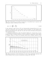
The histograms acc. to Figure 2.23 can be subdivided into two separated
density functions, where the mean values correspond to loaded and unloaded

vehicles. The statistical parameters of these distribution functions are given in
Table 3.6. For the vehicle of Type 3 the distributions are shown examplarily in
Figure 2.25. Furthermore for the development of the load model the frequency
of the different vehicle types in the lanes 1 and 2 is needed. The records based
on the Auxerre traffic are given in Figure 2.25.
The number of axles per vehicle varies widely depending on the differ-
ent vehicle manufactures. Nevertheless the frequency distributions of the axle
50 2 Damage-Oriented Actions and Environmental Impact
Table 2.4. Relation between gross weight of the heavy vehicles and the axle weights
of the lorries of types 1 to 4 in % (mean values and standard deviation)
Axle 1 Axle 2 Axle 3 Axle 4 Axle 5 Type of
vehicle
m
V
m
V
m
V
m
V
m
V
G
o
50,0 8,0 50,0 8,0Type 1
G
l
35,0 7,0 65,0 7,0
G
o

40,5 8,4 36,2 8,8 23,7 7,3Type 2
G
l
29,4 5,7 42,8 4,2 27,8 5,3
G
o
30,6 5,8 27,5 4,4 16,2 3,6 13,6 3,1 12,1 3,1Type 3
G
l
17,1 2,4 26,9 4,4 19,9 3,0 19,0 2,8 16,7 3,8
G
o
31,7 5,7 31,3 5,8 13,4 4,1 13,7 3,5 9,9 3,3Type 4
G
l
18,5 4,1 29,1 4,2 18,9 3,6 18,3 3,4 15,2 4,3
Table 2.5. Distance of axles in [m] of the different types of vehicles (mean values
and standard deviation)
Axle 1-2 Axle 2-3 Axle 3-4 Axle 4-5 Type of
vehicle
m
V
m
V
m
V
m
V
Type 1
3,71 1,1

Type 2
3,78 0,71 1,25 0,03
Type 3
3,30 0,26 4,71 0,78 1,22 0,13 1,23 0,14
Type 4
4,27 0,40 4,12 0,31 4,00 0,42 1,25 0,03
pacings show three cases with peak values nearly constant and very small
standard deviations (vehicles of types 2, 3 and 4 with a space of 1.3 m corre-
sponding to double and triple axles and with a space of 3.2 m corresponding to
tractor axles of the articulated lorries). For the other spacings widely scattered
distributions were recorded resulting from the different construction types of
vehicles.
As mentioned before, the traffic data given in Figures 2.23 and 2.24 are
based on the traffic records of the Auxerre traffic in France. These data gave
no sufficient information about the distribution of gross vehicle weight G on
the single axles. Additional information from the traffic records of the Brohltal
-Traffic in Germany (Highway A61) was used to define single axles weights
and the spacing of the axles. These data (mean values of axle weight and
axle spacing and corresponding standard deviations) are given in Tables 3.7
and 3.8.
A further important parameter is the description of different traffic situa-
tions. For the development of load models the normal free flowing traffic as
2.3 Transport and Mobility 51
a[m]
200
400 600
0,001
0,002
0,003
0,004

0,005
f(a)
90
D
)1( DO
a[m]
f(a)
20
100
Fig. 2.26. Comparison of measured and theoretical values for the density function
of intervehicle distances
well as condensed traffic and traffic jam have to be distinguished. The main
parameters of the probability density functions for the distance are the lorry
traffic density per lane (lorries per hour), the ratio between lorries and mo-
torcars, the mean speed and the probability of occurrence of lorry distances
less than 100 m to cover the development of convoys.
A typical example for the distribution of distances measured at motorway
A7 near Hamburg is given in Figure 2.26 and compared with an analytical
function for high traffic densities given in [720]. The density function is ap-
proximated by a linear increase up to 20 m due to the minimum distance, a
constant part up to a distance of 100 m because of convoys and an exponen-
tially decreasing part for distances greater than 100 m for covering free flowing
traffic. Another possibility is the approximation of the intervehicle distance
by a log-normal distribution [305] which is based on new traffic data [314].
In Figure 2.26 the value α of the constant part between 20 and 100 m,
giving the probability of occurrence for lorry distances less than 100 m, and
the value λ were obtained from traffic records of 24 representative traffics
in Germany. Additional information regarding the probability of occurrence
of convoys are given in [267]. These accurate models apply mainly to the
development of fatigue load models. Regarding load models for ultimate and

serviceability limit states simplified models for the vehicle distances can be
used on the safe side. In case of flowing traffic the distance between lorries is
given by a minimum distance required, which results from a minimum reaction
time of a driver to avoid a collision with the front vehicle in case of braking.
OnthesafesideaminimumbrakingreactiontimeT
s
of the driver of one
second is assumed. Then the minimum distance a is given by a = v · (T
s
)
where v is the mean speed of the vehicles. With this assumption also convoys
are covered. The distance is limited to a minimum value of 5 m in case of jam
situations.
52 2 Damage-Oriented Actions and Environmental Impact
2.3.1.3 Basic Assumptions of the Load Models for Ultimate and
Serviceability Limit States in Eurocode
As mentioned before, the load model in Eurocode 1 is mainly based on the
traffic records of the A6 motorway near Auxerre with 2 × 2 lanes because
these measurements were performed over long time periods in both lanes of
the Highway and because these data represent approximately the current and
future European traffic with a high rate of heavy vehicles related to the total
traffic amount and also with a high percentage of loaded heavy vehicles (see
also Figure 2.24). The European traffic records had been made on various
locations and at various time periods. For the definition of the characteristic
values of the load model therefore the target values of the traffic effects have to
be determined. For Eurocode 1-2 it was decided, that these values correspond
to a probability p = 5% of exceeding in a reference period R
T
=50years
which leads to a mean return period of 1000 years.

For the determination of target values of the traffic effects additional as-
pects have to be considered. The measurements of the moving traffic (e.g. by
piezoelectric sensors) include some dynamic effect depending on the rough-
ness profile of the pavement and the dynamic behaviour of the vehicles which
has to be taken into account for modelling the traffic. The dynamic effects
of the vehicles can be modelled acc. to Figure 2.27 taking into account the
mass distribution of the vehicle, the number and spacing of axles, the axle
characteristic (laminated spring, hydraulic or pneumatic axle suspension), the
damping characteristics and the type of tires [720, 530, 238, 99, 330, 331]. The
normal surface roughness can be modelled by a normally distributed station-
ary ergodic random process. The roughness is a spatial function h(x) and the
relation between the spatial frequency Ω and the wave length L is given by
Ω =2π/L [1/m]. In the literature many surfaces have been classified by power
spectral densities Φ
h
(Ω) acc. to Figure 2.27. Increasing exponent w results in
a larger number of wave length and increasing Φ
h
(Ω) results in larger ampli-
tudes of h(x). For modelling the surface roughness of road bridges w =2can
be assumed. The quality of the pavement of German roads can be classified
for motorways as ”very good”, for federal road as ”good” and for local roads
as ”average”.
While for the global effects of bridge structures an average roughness profile
can be assumed, for shorter spans up to 15 m local irregularities (e.g. located
default of the carriageway surface, special characteristics at expansion joints
and differences of vertical deformation between end cross girders and the
abutment) have to be taken into account. These irregularities were modelled
in Eurocode 1-2 by a 30 mm thick plank as shown in Figure 2.27.
As mentioned above, the axle and gross weights of the vehicles of the Aux-

erre traffic were measured by piezoelectric sensors. The calculations with fixed
base and the vehicle model acc. to Figure 2.27 showed for good pavement
quality, that the characteristic values determined from the measured gross
and axle weights include a dynamic amplification of approximately 15% of
2.3 Transport and Mobility 53
S
x
z
M
m
A
,T
A
spring and damper
of the vehicle body
mass of the axle
spring and damper
of the tyre
h(x)
unevenness of the
carriageway
200
200
300
30
Model for irregularities
Modelling of the vehicles
10
2
10

1
10
0
10
-1
10
-2
spatial frequency :=2S/L [m
-1
]
power spectral density )
h
(: ) [cm
-3
]
10
2
10
1
10
0
10
-1
10
-2
10
3
10-
3
PSD- spectras acc. to ISO-TC 108

a
ve
r
a
ge
pa
ve
me
n
t
)
h
(
:
o
)=16
go
o
d
pa
v
e
me
nt
)
h
(
:
o
)

=4
ve
r
y goo
d pave
m
e
nt
)
h
(
:
o
)
=
1
w
o
ohh
)()(

»
¼
º
«
¬
ª
:
:
:) :)

:
o
=1 m
-1
w=2
+h
-h
+x[m]
L
Fig. 2.27. Model for the vehicles and local irregularities and power spectral density
of the pavement
the axles weights and 10% of the vehicle gross weight. The filtering of the
dynamic effects leads in comparison to the measured values to a reduced stan-
dard deviation. The corrected data of the static vehicle weights are given in
Table 3.9. The dynamic behaviour of the bridge structure is mainly influ-
enced by the span length and the dynamic characteristics of the structure
[169] (eigenvalues acc. to Figure 2.28 and the damping characteristics). With
the vehicle model and the modelling of the roughness of pavement surface acc.
Table 2.6. Statistical parameters of the corrected static traffic records of Auxerre
(1986)
mean value P of the total
vehicle weight [kN]
standard deviation V
[kN]
lane 1 lane 2 lane1 lane 2
Type 1 G
o
G
l
74

183
64
195
31
23
29
28
Type 2 G
o
G
l
123
251
107
257
40
31
39
35
Type 3 G
o
G
l
265
440
220
463
51
42
68

65
Type 4 G
o
G
l
254
429
196
443
37
55
60
64
54 2 Damage-Oriented Actions and Environmental Impact
span length in [m]
10 20 30 40 50 60
70
80 90
2
4
6
8
10
Hz81,0
L
1
4,95f
933,0
r V
f [Hz]

Eigenvalues
(1. mode)
Comparison of calculated
and measured dynamic
amplification
10 20 30 40
50
60
70
80
vehicle speed [km/h]
calculated values
measured values
dynamic amplification in [%]
10
20
30
40
50
60
70
36,95
41,0m
32,35
Fig. 2.28. Measurements of the eigenvalues of the first mode of steel and concrete
Bridges [169], and comparison of theoretically determined dynamic amplifications
with measurements
to Figure 2.27 results can be obtained by dynamic calculations of the bridge
and be compared with measurements at bridges. Figure 2.28 shows an exam-
ple of the calculated and measured dynamic amplification of the Deibel-Bridge

[720].
With the assumptions and models explained above, a realistic determina-
tion of the dynamic and static action effects due to traffic loads is possible. In
a first step random generations of load files and roughness profiles of the pave-
ment surface can be produced. Each load file consists of lorries with distances
based on constant speed per lane. The main input parameters are the number
and types of lorries, the probability of occurrence of each lorry type, the his-
togram of the static lorry weights of each type, the distribution of lorries to
several lanes. For the load files simply supported and continuous bridges with
one, two and four lanes and different span lengths between 1 and 200 m with
a representative dynamic behaviour (mass, flexural rigidity, mean frequency
acc. to Figure 2.28 and damping) have to be investigated in order to get re-
sults which are representative for the dynamic amplification of action effects
of common bridges. Three different types of bridges with cross-sections with
one, two and four lanes were investigated for the load model in Eurocode 1-2.
For the different lanes the traffic types acc. to 3.10 were assumed, where
traffic type 1 is a heavy lorry traffic for which motorcars were eliminated from
the measured Auxerre traffic. The traffic type 2 is the measured traffic of lane
2.3 Transport and Mobility 55
Table 2.7. Different cross-sections and traffic types for the random generations
number of
lanes
type of cross section traffic types of the different lanes
1
3,0 m
Type 1
2
3,0 m
3,0 m
Lane 1: Type 1

Lane 2: Type 2
4
3,0 m
3,0 m
3,0 m
3,0 m
Lane 1: Type 1
Lane 2: Type 3
Lane 3:Type 3
Lane 4: Type 2
1 in Auxerre, including motorcars and traffic type 3 is the measured traffic of
lane two in Auxerre. Detailed information about the generation of these load
files are given in [720, 530].
With random load files the static and the dynamic action effects of the
different bridge types can be determined. The comparison of the static and
dynamic action effects gives information about the dynamic amplification and
the dynamic factor Φ, influenced by the dynamic behaviour of the lorries,
the bridge structure and by the quality of the pavement. The results of the
simulations can be plotted in diagrams which give the cumulative frequency of
the action effects. A typical example is given in Figure 2.29 for a bridge with
50
97
99,9
M
E
[kNm]
1000
1300
700
convoy v= 80 km/h

convoy v= 60 km/h
convoy v= 40 km/h
traffic jam
cumulative frequency [%]
action effect
M
E
Fig. 2.29. Cumulative frequency of the action effects for different vehicle speeds
[530]
56 2 Damage-Oriented Actions and Environmental Impact
1,2
1,4
1,6
1,8
1,0
0,8
2,0
2,2
10 20 30 40 50 60 70 80
L [m]
flowing traffic and good pavement quality
flowing traffic and average pavement quality
pavement irregularities (30 mm thick plank)
M
Fig. 2.30. Influence of the quality of the pavement on the dynamic amplification
factor ϕ[530]
one lane, good pavement quality and a span of 20 m. It can be seen that for
this example the increase of the vehicle speed leads also to an increase of the
dynamic action effects. Furthermore the dynamic amplification is extremely
influenced by the roughness of the pavement and also by the span of the

bridge. The influences of the pavement quality and traffic in more than one
lane are shown in Figures 2.30 and 2.31. The results of the simulations show for
condensed traffic no significant influence of the span length and the number
of loaded lanes on the dynamic amplification. In case of flowing traffic the
dynamic amplification of action effects depends significantly on the quality of
the pavement, the number of loaded lanes, the span length and the type of
the influence line of the action effect considered.
1,2
1,4
1,6
1,8
510 15 20 25 3035
1,2
1,4
1,6
1,8
M
10 20 30 40 50 60 70 80
L [m]
L [m]
bending moment
vertical shear
bending moment
M
Fig. 2.31. Influence of the span length and the number of loaded lanes on the
dynamic amplification factor ϕ
2.3 Transport and Mobility 57
200
200
300

30
Model for irregularities
1,0
1,1
1,2
1,3
L[m]
51015202530
'M
Fig. 2.32. Additional dynamic factor Δϕ taking into account irregularities of the
pavement [9]
Figure 2.31 shows the envelope of the calculated dynamic factors ϕ for flow-
ing traffic as a function of the span length. For the development of the load
model in Eurocode 1-2 it was decided, that the dynamic amplification of the
action effects should be included in the load model because otherwise different
parameters like the traffic situation (flowing traffic or traffic jam, the qual-
ity of the pavement, the number of loaded lanes and the type of the influence
line) had to be considered separately. The calculations show additionally, that
the dynamic amplification due to flowing traffic is only relevant for shorter
span length up to 50 m because for greater span length the condensed traffic
with low vehicle spacings or the traffic jam lead to extreme action effects. As
explained above the dynamic effects due to local irregularities were modelled
by a 30 mm thick plank, which leads especially for shorter spans to a signifi-
cant additional dynamic amplification factor. Figure 2.32 gives the additional
dynamic factor Δϕ due to irregularities which has to be considered especially
for fatigue verifications for short spans, e.g. for end cross girders and members
near expansion joints (see Figure 2.32).
With the random load files the static and the dynamic action effects and
the characteristic values of the action effects can be determined. As mentioned
above, the characteristic values in Eurocode 1-2 correspond to a probability

p = 5% of exceeding in a reference period R = 50 years which leads to a
return period of T
R
= 1000 years. The procedure for the determination is
shown in Figure 2.33. The simulation of different bridge types gives a cu-
mulative frequency of the considered action effects. The characteristic values
can be determined by extrapolation. Finally these characteristic values can
be compared with a simplified characteristic load model.
The load model for global effects in Eurocode 1-2 [9] consists of uniformly
distributed loads and simultaneously acting concentrated loads, so that global
effects in large spans and the local effects in short spans can be covered by
58 2 Damage-Oriented Actions and Environmental Impact
static values of
simulations
99,9999
99,90
99,00
50,00
action effect
M
E
dynamic values
of simulations
extrapolation for the
determination of the
characteristic values
E
k,dyn
E
k,stat.

influence line
for M
E
dynamic
amplification factor:
M
E
.stat,k
dyn,k
E
E
I
cumulative frequency [%]
Fig. 2.33. Determination of the characteristic values of the action effects from the
random generations of loads
the same model taking into account the dynamic amplification, where average
pavement quality is expected. The carriageway with the width w is measured
between kerbs or between the inner limits of vehicle restraint systems. For the
notional lanes a width of w
l
= 3,0 m is assumed, and the greatest possible
number n
l
of such lanes on the carriageway has to be considered. The locations
of the notional lanes are not be necessarily related to their numbering. The
lane giving the most unfavourable effect is numbered as Lane Number 1, the
lane giving the second most unfavourable effect is numbered as Lane Number
2 and so on. For each individual verification the load models on each notional
lane and on the remaining area outside the notional lanes have to be applied
on such a length and longitudinally located so that the most adverse effect is

obtained.
The Load Model 1 in Eurocode 1-2 is shown in Figure 2.34. It consists
of a double axle as concentrated loads (Tandem System TS) and uniformly
distributed loads (UDL-System). For the verification of global effects it can be
assumed that each tandem system travels centrally along the axes of notional
lanes. For local effects the tandem system has to be located at the most
unfavourable location and in case of two neighbouring tandem systems they
have to be taken closer, with a distance between wheel axles not smaller
than 0,5 m. With the adjustment factors α
Qi
and α
qi
the expected traffic on
different routes can be taken into account.
The last step in the development of the load model is the comparison of
the characteristic action effects caused by the normative load model with
the characteristic values of the dynamic values of the real traffic simulations.
Figure 2.35 shows this comparison for a three span bridge girder with one,
two and four lanes.
For the verification of local effects a Load Model 2 is given in Eurocode
1-2. This model consists of a single axle load equal to 400 kN, where the
2.3 Transport and Mobility 59
Lane number 1:
Q
1k
= 300 kN a
Q1
q
1k
= 9 KN/m²

Lane number 2:
Q
2k
= 200 a
Q2
q
2k
= 2,5 KN/m²
Lane number 4 and further
lanes as well as remaining
areas:
a
Q3
q
3k
= 2,5 KN/m²
0,50
2,00
0,50
0,50
2,00
0,50
D
Qi
Q
ik
D
qi
q
ik

2,00m
>
0,50m
2,00m
1,20m
D
Qi
Q
ik
w
1
w
2
w
3
0,4 m
0,4 m
contact area of the
wheel loads
0,50
2,00
0,50
Lane number 3:
Q
3k
= 100 a
Q2
q
2k
= 2,5 KN/m²

w
i
Application of the
Tandem System for
local verifications
Application of the Tandem System for global
verifications
Fig. 2.34. Load Model 1 according to Eurocode 1-2
100
20
40
60 80
200
300
400
500
M
E
/L
span length
L
L
L
L
M
E
Load Model 1 acc. to Eurocode 1
simulation
Fig. 2.35. Comparison of the Load Model 1 in Eurocode -2 with the characteristic
values obtained from real traffic simulations

dynamic amplification for average pavement quality is included. In the vicinity
of expansion joints an additional dynamic amplification has to be applied for
60 2 Damage-Oriented Actions and Environmental Impact
Table 2.8. Traffic data of different locations and characteristic values of gross and
axle weight [720]
country location year
number n
l
of lorries
per day
weight of
one axle
kN
tandem
axles
kN
tridem
axles
kN
gross weight
of vehicle
kN
Germany Brohltal 1984 4793 211 357 434 853
Belgium Chamonix 1987 1204 192 355 480 724
France Auxerre 1986 2630 245 397 527 811
France Angers 1987 1272 192 340 456 670
France Lyon 1987 1232 267 450 475 930
Table 2.9. Different design situations and corresponding return periods and fractiles
Design situation Return period T
R

Fractile of the
distribution of
action effects in
%
infrequent 1 year 99,997
frequent 1 week 99,891
quasi - permanent 1 day 99,240
taking into account the local irregularities at expansion joints. The contact
surface of each wheel can be taken into account as a rectangle of sides 0,35 m
and 0,6 m.
The evaluation of the traffic data of different locations lead to static char-
acteristic axle values Q
k
given in Table 3.11, where the characteristic values
relate to a return period T
R
of 1000 years (probability p of 5% in 50 years).
It can be seen that the characteristic values are depending on the location.
Taking into account the dynamic amplification for short spans (see Figure
2.31), this leads to the axle weight given in Eurocode 1-2.
For serviceability limit states like limitation of deflections, crack width con-
trol and limitation of stresses to avoid inelastic behaviour, different design
situations have to be distinguished. The Eurocodes distinguish between in-
frequent, frequent and quasi permanent design situations characterised by
different return periods. The return periods and the corresponding fractile of
the distribution of the dynamic action effects are given in Table 3.12.
A change of the return period is equivalent with a change of the fractile of
the distribution (see Figure 2.36). The representative values F
rep
of the action

effects can then be written as F
rep
= ψF
k
,whereF
k
is the characteristic value.
As explained above, the characteristic values were determined with ad-
verse assumptions regarding the quality of the pavement Φ(Ω
h
) = 16 acc. to
2.3 Transport and Mobility 61
static values of
simulations
99,9999
99,90
99,00
50,00
action effect E
dynamic values
of simulations
characteristic values E
k
E
k,dyn
E
k,stat.
dynamic
amplification factor
M

E
.stat,k
dyn,k
E
E
I
cumulative frequency [%]
representative
valuesE
rep
=\ E
k
.stat,rep
dyn,rep
E
E
I
representative values:
characteristic values:
E
rep,stat.
E
rep,dyn.
Fig. 2.36. Determination of the representative values and the corresponding dy-
namic factors
10 20 30
40
50 60 70 80
0,2
0,4

0,6
0,8
1,0
L[m]
<
TR
L
L
L
condensed traffic and
traffic jam (v= 10km/h)
flowing traffic
(v= 80km/h)
M
E
2 lanes
4 lanes
Fig. 2.37. Factors ψ
TR
for frequent design situations acc. to [37] for average pave-
ment quality with Φ(Ω
h
)=16
Figure 2.27, the composition of the traffic (100% lorries in the first lane) and
a probability of traffic jam of 100%. The combination values taking into ac-
count these assumptions lead to values Ψ
TR
, which only cover the influence of
the return period T
R

. Figure 2.37 shows an example for the frequent design
situation [37] for average pavement quality. It can be seen that the values
Ψ
TR
are dependent on the span length, the traffic situation and the number
of lanes. The condensed traffic and traffic jam give the greatest values Ψ
TR
.
The values Ψ
TR
can be reduced by additional factors to be more close to
reality. As mentioned before the quality of the pavement has a significant
influence on the dynamic action effects. On the basis of a good pavement
quality with Φ(Ω
h
) = 4 acc. to Figure 2.27 which can be assumed e.g. for
62 2 Damage-Oriented Actions and Environmental Impact
10 20 30
40
50 60 70 80
0,2
0,4
0,6
0,8
1,0
<
TR
L
L
L

M
E
L[m]
flowing traffic
(v= 80km/h)
condensed traffic and
traffic jam (v= 10km/h)
average pavement quality
)(:
h
) =16
good pavement quality
)(:
h
) =4
Fig. 2.38. Influence of the pavement quality on the factor Ψ
TR
for frequent design
situations
highways and federal roads in Germany, a reduction factor for the dynamic
action effects of Ψ
Ω
≈ 0.89 results from the simulations. The influence of the
pavement quality is shown in Figure 2.38 as a function of the span length.
A second reduction factor covers the influence of the probability of traffic
jams. Based on the evaluations in [267] with a rate of ν =3× 10
−3
traffic
jams per kilometre and day a percentage of traffic jam of 6% to 9% of the
annual traffic results in comparison with the Auxerre traffic. This leads to the

reduction factor Ψ
ν
≈ 0.95. A further reduction factor Ψ
v
covers the effect of
the realistic traffic composition (percentage of the lorry on each lane). For a
mean rate of 32% of lorries related to the total traffic the factor Ψ
v
for bridges
with one lane is approximately 0.9 for a return period of 1 week and 0.96 for
a return period of 1 year. For bridge structures with two lanes values of 0.74
and 0.76 result from the calculations in [530, 37].
With the additional reduction factors values Ψ = Ψ
TR
Ψ
Ωh
Ψ
ν
result which
are in the range of 0.8 for the infrequent and 0.7 for the frequent design
situations of bridges with small spans up to 40 m where the single axle loads
dominate the actions effects. For spans exceeding 40 m the flowing traffic with
mainly uniform distributed loads gives values Ψ ≈ 0.8 for the infrequent and
0.45 for frequent design situations. These values correspond to the values in
Eurocode 1-2 (Table 3.13).
2.3.1.4 Principles for the Development of Fatigue Load Models
Fatigue is the progressive, localized and permanent structural change occur-
ring in materials subjected to fluctuating stresses initiating and propagating
cracks through a structural part after a sufficient number of load cycles. Fa-
tigue is induced in bridges mainly by heavy vehicles. The development of

appropriate load models and verification concepts is a main topic in modern
2.3 Transport and Mobility 63
Table 2.10. Factors Ψ for the determination of the representative values for ser-
viceability limit states acc. to [9]
Load Model 1 Load Model 2
tandem system
uniform distributed
loads
single axle
infrequent design
situations
0,8 0,8 0,8
frequent design
situations
0,75 0,4 0,75
quasi permanent
design situations
0 0 0
bridge design. As mentioned above the load model in Eurocode 1-2 is based on
the Auxerre traffic which covers heavy European continental traffic. Therefore
also for the fatigue load models in Eurocode 1-2 the Auxerre traffic was used
for the pre-normative investigations. For typical bridges, random files of the
traffic loads, the traffic flow and the intervehicle distances were produced for
the determination of the dynamic action effects, which take into account the
pavement quality and the dynamic behaviour of the vehicles and the bridge
structure (Figure 2.39). From this calculation the time history of stresses or
internal forces is obtained and with the rainflow-counting or reservoir method
[201] the spectrum of the action effects can be determined. The next step is
the determination of the damage accumulation based on given fatigue strength
curves based on a damage accumulation hypothesis.

For steel structures and for reinforcement and prestressing steel the fatigue
strength curves acc. to Figure 2.40 can be used, where the fatigue strength
curve for steel structures [30] is defined by the fatigue strength category (fa-
tigue strength at two millions cycles) and the constant amplitude fatigue limit
Δσ
D
at 5 million cycles. For stress ranges above Δσ
D
the slope m of the curve
in a double logarithmic scale is equal 3 and for stress ranges less than Δσ
D
a
slope m = 5 can be assumed. The fatigue strength curves were derived from
international evaluations of fatigue tests with large scale test specimen. For
stress ranges of the design spectrum which are below the cut-off limit Δσ
L
at
10
8
load cycles it may be assumed that these stress ranges do not contribute
to the calculated cumulative damage. Typical examples for fatigue strength
categories in steel and composite bridges are shown in Figure 2.41. The fatigue
strength curves in Figures 2.40 and 2.41 relate to nominal stresses.
For steel reinforcement bars the fatigue strength curve is given in [28, 437]
and described by a two linear function in the double logarithmic scale without
any constant amplitude fatigue limit (Figure 2.40). While for steel structures
normally a linear relation can be assumed between the fatigue loading and the
stresses, for concrete structures the non linear behaviour due to cracking of con-
crete has to be taken into account for the determination of the time history of
the stresses. In this case in addition to the fatigue loading also the dead load

and effects due to climate temperature actions have to be considered [437].
64 2 Damage-Oriented Actions and Environmental Impact
V
'V
'V
1
'V
2
'V
3
'V
4
n
1
n
2
n
3
n
4
stress range spectrum
influence line for the
stress V
i
traffic loading and traffic composition
time t
'V
1
'V
2

'V
3
'V
4
stress history of the dynamic
action effects and cycle counting
(e.g. reservoir or rain flow
method)
N
'V(log)
'V
i
n
i
N
Ri
N (log)
damage accumulation
0,1
N
n
DD
Ri
i
i
d
¦¦
stress V
i
fatigue strength curve

Fig. 2.39. Determination of stress spectra and damage accumulation due to fatigue
loading
'V
R
(log)
N
R
(log)
N
c
N
D
N
L
'V
c
'V
D
'V
L
m
1
=3
m
2
=5
'V
C
- Detail Category N
C

= 2 · 10
6
'V
D
- Constant amplitude fatigue limit N
D
= 5 · 10
6
'V
L
- Cut off limit N
L
= 10
8
1
m
Fatigue strength curves for
structural steel
Fatigue strength curves for
reinforcement and
prestressing steel
N
R
(log)
'V
R
log)
1
m
'V

Rsk
N*
m
1
m
2
5358,510
7
welded bars and
wire fabric
533510
7
splicing devices
95162,510
6
straight bars
m
2
m
1
'V
Rsk
at N*
cycles
[N/mm
2
]
N*
type of
reinforcement

i
m
1
i
D
DRi
N
N
»
¼
º
«
¬
ª
V' V'
i
m
1
i
Rski,Rs
N
N
»
¼
º
«
¬
ª
V' V'


Fig. 2.40. Fatigue strength curves for structural steel and reinforcement
The main issues in the development of fatigue load models is the dam-
age accumulation hypothesis. In civil engineering normally a linear damage
2.3 Transport and Mobility 65
'V
'V
Category 80
'V
c
= 80 N/mm
2
'V
'V
1
2
3
1
2
3
4
4
L
L
L
'V
'V
'V
Category 125
'V
c

= 125 N/mm
2
automatic butt weld carried out
from both sides
Category 56
'V
c
= 56 N/mm
2
for L>100mm
>10mm
Category 71
'V
c
= 71 N/mm
2
for Ld 50mm
'V
Fig. 2.41. Typical examples for fatigue strength categories
accumulation according to Miner [543] is used (Figure 2.40). Based on this
assumption a realistic fatigue load model must fulfil the condition, that the
cumulative damage produced by the real traffic must be equal to the cumula-
tive damage caused by the load model. The main parameters which have to be
considered are the design fatigue life, the type and number of lorries crossing
the bridge, the traffic composition and the number of lanes with heavy traffic
and in addition the quality of the pavement and the dynamic behaviour of
the vehicles and the bridge. For fatigue problems of bridges only the traffic
situation of flowing traffic has to be considered because the number of traffic
jams is negligible during the design life. Furthermore the influence of motor-
cars can be neglected, because the stress ranges caused by motorcars do not

reach the cut off limit of the fatigue strength curves.
For the development of fatigue load models further considerations are nec-
essary. For Eurocode 1-2 e.g. it was decided that the load model should include
the dynamic amplification of the real traffic. Regarding the modelling several
strategies are possible. One possibility is to consider only one type of vehicle
in verifications and to take into account all other effects resulting from the
real traffic by damage equivalent factors. This is the basis of the Load Model
3 in Eurocode 1-2. An other possibility is the definition of a set of lorries
which together produce effects equivalent to those of typical traffic on Euro-
pean roads. An example for such a model is the Load Model 4 in Eurocode 1-2
(Figure 2.42). The fatigue models 3 and 4 are intended to be used for fatigue
life verifications by reference to a fatigue strength curve. For the fatigue life
verification it has to be distinguished between different traffic categories. The
category is defined by the number of slow lanes, the number N
obs
of heavy
vehicles with a maximum gross weight more than 100 kN which was observed
66 2 Damage-Oriented Actions and Environmental Impact
Table 2.11. Traffic categories acc. to Eurocode 1-2
Traffic category
N
obs
per year and per slow
lane
1
Roads and motorways with 2 or more lanes per direction with
high flow rates of lorries
2,0 x 10
6
2

Roads and motorways with medium flow rates of lorries 0,5 x 10
6
3
Main roads with low flow rates of lorries 0,125 x 10
6
4
Local roads with low flow rates of lorries 0,05 x 10
6
or estimated per year and per slow lane. Typical traffic categories acc. to
Eurocode 1-2 are given in Table 3.14.
Fatigue Load Model 4 in Eurocode 1-2 consists of a set of standard lorries
(Figure 2.42) which together produce effects equivalent to those of typical
traffic on European roads. This model is intended to determine stress range
spectra resulting from the passage of lorries on bridge. The equivalent lorries
are defined by the number of axles and the axle spacing, the equivalent load
of each axle, the contact surface of the wheels, the transverse distance of the
wheels and the percentage of each standard lorry in the traffic flow.
For the verification of global action effects the model can be placed centrally
on the notional lanes acc. to Figure 2.34. For local members (e.g. concrete slabs
or orthotropic decks) the model has to be centred on notional lanes assumed
to be located anywhere on the carriageway. Where the transverse location of
the fatigue load model is significant for the action effects e.g. in orthotropic
decks, a statistical distribution of this transverse location acc. to Figure 2.43
has to be taken into account.
As mentioned above, the fatigue load models in Eurocode 1-2 include a
dynamic load amplification ϕ
fat
. An additional dynamic load amplification
factor Δϕ
fat

acc. to Figure 2.43 has to be taken into account near expansion
joints to allow for the effects of local irregularities in this regions. For the other
regions of the bridge the dynamic load amplification factor must take into
account the high number of relative small load cycles. This can be achieved by
introducing a damage equivalent dynamic amplification factor acc. to Figure
2.44 which results from the comparison of the cumulative damage calculated
with and without dynamic amplification of the Auxerre traffic. The procedure
for the determination of ϕ
fat
is shown in Figure 2.44. Because most of the
stress ranges are below the fatigue strength limit Δσ
D
, the dynamic factor
can be determined withaconstantvalueofm = 5 for the slope of the fatigue
strength curve.
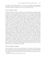
In Eurocode 1-2 good pavement quality acc. to Figure 2.27 was assumed.
The influence of the pavement quality on the dynamic amplification factor
ϕ
fat
can be seen from Figure 2.45. For good pavement qualities the dynamic
2.3 Transport and Mobility 67
traffic type and lorry percentagevehicle type
local
traffic
medium
distance
long
distance
axle
loads

[kN]
axle spacing
[m]
Lorry
A
B
C
C
C
5510
70
130
90
80
80
4,80
3,60
4,40
1,30
A
B
B
B
51515
70
140
90
90
3,40
6,00

1,80
A
B
C
C
C
53050
70
150
90
90
90
3,20
5,20
1,30
1,30
A
B
B
5105
70
120
120
4,20
1,30
A
B
804020
70
130

4,50
wheel type
320
220
320
220
220
320
270
2,0 m
Type A
Type B
Type C
x
wheel types and dimensions of the wheel contact
surface in mm
Fig. 2.42. Set of lorries of Fatigue Load Model 4 in Eurocode -2 and contact surfaces
of the wheels
'M
fat
1,3
1,2
1,1
1,0
6,04,02,0
D [m]
D
5 x 0,1 m
50%
18%

7%
Distribution of transverse location of
centre line of vehicle
Dynamic load amplification factor
near expansion joints
Fig. 2.43. Distribution of transverse location of centre line of vehicles and dynamic
load amplification factor near expansion joints
68 2 Damage-Oriented Actions and Environmental Impact
10
5
10
6
10
7
10
8
10
9
10
100
'V(log)
N(log)
'V
i
category 160
category 36
Di
m
C
i

CRi
i
i
for
N
1
N
n
D
1
V'tV'
»
¼
º
«
¬
ª
V'
V'

damage:
Linear damage accumulation:
¦
d 0,1DDD
Auxerrei
LiD
m
D
i
DRi

i
i
for
N
1
N
n
D
2
V'tV'tV'
»
¼
º
«
¬
ª
V'
V'

Lii
for0D VV'
i
m
1
i
D
DRi
N
N
»

¼
º
«
¬
ª
V' V'
N
L
N
D
N
C

i
i
i
i
i
i
m
stat,Auxerre
dyn,Auxerre
m
m
stat,i
stat,i
m
dyn,i
dyn,i
fat

m
statfatstat,i
m
dyn,i
dyn,i
D
D
n
n
nn
V'
V'
MV'M V'
¦
¦
¦
¦
Damage equivalent dynamic amplification factor:
Fig. 2.44. Linear damage accumulation and damage equivalent dynamic amplifica-
tion factor ϕ
fat
1,0
1,2
1,4
1,6
1,8
10 20 30 40 50 60 70 80
L [m]
L
L

L
M
E
M
fat
good pavement
quality )
h
(:
o
)=4
average pavement
quality )
h
(:
o
)=16
flowing traffic with v= 80 km/h
Fig. 2.45. Influence of the pavement quality on the damage equivalent dynamic
amplification factor [530]
factor ϕ
fat
is in the range of 1.2, which is included in the load model in Figure
2.44. For average pavement qualities a mean increase in the range of 20% was
obtained which leads to an increase of the damage D byafactorof2.5and
a decrease of the fatigue life to 0.4 when for the slope of the fatigue strength
curve m = 5 is assumed. This demonstrates that the authorities have the
responsibility for a careful maintenance of the roads.
As mentioned above, Fatigue Load Model 3 (Figure 2.46) consists of a
single vehicle with four axles, each of them having two identical wheels with a

squared surface contact area of each wheel with the side lenght of 0.4 m. The
weight of the axles is equal to 120 kN and includes the dynamic amplification
factor ϕ
fat
. The damage of the real traffic is taken into account by a damage
2.3 Transport and Mobility 69
1,20m
1,20m
6,00 m
2,00 m
3,00 m
0,4 m
0,4 m
Axle loads of Fatigue
Load Model 3
120 kN 120 kN 120 kN
120 kN
lane width
Fatigue verification
fat,M
C
LMfat,F
J
V'
dV'OJ
'V
C
'V
LM
O'V

LM
N
C
N
D
'V
i
(n
i
)
fatigue strength curve
Fig. 2.46. Fatigue Load model 3 in Eurocode 1-2 and fatigue verification for steel
structures
equivalent stress range λ · Δσ
LM
[31, 327] with λ = λ
1
· λ
2
· λ
3
· λ
4
≤ λ
max
The factor λ
1
takes into account the damage effect of traffic depending on the
length of the critical influence length, λ
2

is a factor for the traffic volume, λ
3
allows for different design life and λ
4
takes into account the traffic on other
lanes. The fatigue verification can then be performed according to Figure 2.46,
where Δσ
LM
is the stress range caused by the load model, Δσ
C
is the reference
strength at 2 million load cycles and γ
F,fat
and γ
M,fat
are the partial safety
factors for the equivalent constant amplitude stress λ ·Δσ
LM
and the fatigue
strength Δσ
C
.
The damage equivalent factors must be determined from the real traffic,
where for Eurocode 1-2 the Auxerre traffic was used. In a first step it is
assumed that for the determination of λ
1
the factor λ
2
is equal to 1.0 for
N

o
=0.5 × 10
6
lorries per year and slow lane and that a design life T
so
=
100 years corresponds to a factor λ
3
= 1.0. Furthermore only one slow lane is
investigated which gives λ
4
= 1.0. Then the factor λ
1
must fulfil the condition,
that the damage of the load model D
LM
is equal to the damage of the Auxerre
traffic D
Auxerre
= ΣD
i
.
For the calculation of λ
1
at first random load files based on the Auxerre
traffic and the corresponding stress range spectra acc. to Figure 2.44 have
to be determined. The corresponding accumulative damage caused by the
number n
Ls
of simulated lorries results in D

Auxerre
= ΣD
i
. As the damage
caused by the load model has to be equal to the cumulative damage D
Auxerre
,
a correction factor λ
e
for the stress range Δσ
LM
of the load model has to be
introduced (see Figure 2.48). For the same number of lorries n
Ls
the equivalent
damage of the load model D
LM
and the factor λ
e
is given by
D
LM
=
n
Ls
N
D

λ
e

· Δσ
LM
Δσ
D

m
λ
e
=
Δσ
D
Δσ
LM
m

N
D
· D
Auxerre
n
LS
(2.55)
70 2 Damage-Oriented Actions and Environmental Impact
0,2
0,4
0,6
0,8
1,0
1,2
1,4

10
20
30 40 50 60 70
80
L [m]
M
E
flowing traffic with v= 80 km/h
O
e
10
20
30 40 50 60 70
80
L [m]
0,2
0,4
0,6
0,8
1,0
1,2
1,4
O
e
L
L
L
M
E
L

L
L
static action effects
dynamic action effects
Fig. 2.47. Example for the damage equivalent factor λ
e
[530]
N
L
'V(log)
N(log)
'V
e
=O
e
'V
LM
¦

Auxerrei
DDD
N
D
m
1
=3
m
2
=5
N

C
n
S
'V
C
'V
LM
'V
i
(n
i
)
O
1
'V
LM
Fig. 2.48. Determination of the damage equivalent factor λ
1
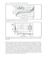
A typical example for the damage equivalent factor for a three span bridge is
given in Figure 2.47. It can be seen that the dynamic amplification leads to
a significant increase of the factor λ
e
. Furthermore the factor depends on the
type of the influence line and the assumption for the quality of the pavement.
The values in Figure 2.47 were determined for a good pavement quality.
For the fatigue verification acc. to Figure 2.46 it has to be taken into account
that the verification is based on the fatigue strength Δσ
C
at N
C

=2×10
6
load
cycles and that in addition the relevant number of lorries during the design
life T
so
is given by N
T O
= N
o
·T
do
. This leads to a further transformation for
the damage equivalent stress range Δσ
e
= λ
e
· Δσ
LM
(see Figure 2.48).
2.3 Transport and Mobility 71
10 20 30 40 50 60 70 80
1,2
1,4
1,6
1,8
2,0
2,2
2,4
2,6

2,8
O
1
10 20 30 40 50 60 70
1,2
1,4
1,6
1,8
2,0
2,2
2,4
2,6
2,8
L [m]
L [m]
O
1
midspan regions
internal supports
L
2,55
1,85
2,0
1,70
2,2
L
1
L
2
L= ½ (L

1
+L
2
)
80
Fig. 2.49. Factors λ
1
for steel bridges given in Eurocode 3-2
Because N
T o
is greater than N
D
in the first step a correction factor α for
the damage equivalent stress related to N
D
is determined using the slope of
the fatigue strength curve m
2
=5.
N
T o
[λ
e
·Δσ
LM
]
5
= N
D
[α · λ

e
·Δσ
LM
]
5
⇒ α =
5

N
T o
N
D
(2.56)
In the second step the transformation of the equivalent stress range related
to N
C
follows using the slope m
1
= 3 (see Figure 2.48)
N
D
[α · λ
e
· Δσ
LM
]
3
= N
C
[α · β ·λ

e
· Δσ
LM
]
3
=
3

N
D
N
C
(2.57)
The damage equivalent factor λ
1
is then given by:
λ
1
= λ
e
· α · β = λ
e
·
5

N
T o
N
D
·

3

N
D
N
C
(2.58)
The equivalent damage factor λ
1
depends on the damage equivalent factor
λ
e
, the type of the fatigue strength curve (slopes m
1
and m
2
and the fa-
tigue strength Δσ
D
and Δσ
D
respectively) and the relevant numbers N
T o
of lorries during the design life assumed for λ
2
= 1.0. Therefore the factor
differs for structures and structural members with different materials (e.g.
structural steel, reinforcement, shear connectors). Figure 2.49 shows the λ
1
-

values for steel bridges which are an envelope of the most adverse values
determined for different types of influence lines. For concrete and composite
bridges corresponding values are given in Eurocode 2-2 [29] and Eurocode 4-2
[31], respectively.
As explained above, the factor λ
1
was determined for the reference value
N
o
=0.5 ×10
6
,whereN
o
corresponds to the traffic category 2 in Table 3.14.
Furthermore for the design life a reference value T
so
= 100 years was assumed.
In case of another traffic category or design life the damage equivalent factor