Lifetime-Oriented Structural Design Concepts- P5 doc

2.3 Transport and Mobility 77
10
2
10
3
10
4
10
5
10
6
10
7
number of vehivles and axles per year
100
200
300
400
500
600
700
800
900
1000
1100
1200
1300
vehicle weight
axle weight
G [kN]
1270 kN

n
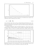
Fig. 2.55. Traffic records from the Netherlands recorded in 2006
periods of one or two years. In this case a further increase of these transports
can be expected and it cannot be excluded that a significant percentage of
these transports is overloaded. A possible increase in the number of such vehi-
cles in combination with a possible overloading has especially to be considered
for the development of future fatigue load models.
A comparable development takes place in other European countries. Figure
2.55 shows the vehicle weight and axle load distributions recorded in 2006 near
the harbour of Rotterdam in the Netherlands. It can be seen that the extreme
values of the gross weight and also the extreme values of the axle loads are
significant higher than the values of the Auxerre traffic (see Figure 2.24).
The shape of the distribution shows that the heavy load transports lead in
comparison with the Auxerre traffic to a new shape of the distribution which
could be taken into account by splitting the distribution into a distribution
for normal traffic and a distribution for heavy load transports.
Additionally the transport industry is extremely interested in new trans-
port concepts at present. In some European countries and also in some Ger-
man federal states field trials take place with modular vehicle concepts, the
so called Giga-Liners with gross weight up to 600 kN and a total length of
25.25 m [314]. Typical vehicles and the corresponding allowable axle loads are
shown in Figures 2.56 and 2.57. These types of vehicles have significant higher
transport capacities and can reduce the transport cost. At present it cannot
be foreseen how the future traffic composition will change. Some people ar-
gue that the new modular concept will reduce the total number of lorries on
roads due to the higher transport capacity. On the other hand it has to be
78 2 Damage-Oriented Actions and Environmental Impact
Vehicles acc. to the modular concept
(gross weight up to 600kN)
25,25 m

16,50-18,25 m
Current trucks in Germany
(gross weight 400kN)
Fig. 2.56. Heavy vehicles on the basis of the modular concept (Giga-Liners)
1,475 5,10 m 1,35 4,65 1,35 5,965 m 1,36
1,36
2,64
1,475 3,215
1,36
5,965 m
1,36
6,27 m
1,36
2,88
1,36
25,25 m
57 kN
74 kN
74 kN
65 kN
65 kN
65 kN
90 kN
90 kN
74 kN
92 kN
92 kN
54 kN
54 kN
78 kN

78 kN
78 kN
Giga – Liner with gross weight of 600 kN
Giga – Liner with gross weight of 580 kN
Fig. 2.57. Axle spacing and allowable axle weights of ”Giga-Liners”
considered that this new type of vehicle can not be loaded on trains, so
that it can be expected that no significant reduction of the total road traffic
will occur. First investigations [201] show that especially for bridges with
longer spans the current European load model has to be modified, when
the percentage of the new vehicles reaches 20% to 40% related to the to-
tal heavy traffic. Furthermore at present no information is available regarding
the driving of such vehicles in convoys, especially on routes with acclivities,
and the possible overloading and wrong loading which can lead to higher
axle weights.
2.3 Transport and Mobility 79
The new traffic concepts and development regarding heavy transports need
new technologies to get more detailed information about the actual traffic
situation and also a more close cooperation between the car industry and the
authorities and experts for the development of realistic traffic models. The
Weight in Motion (WIM) is a technology [407, 588] for the determination of
the weight of vehicles without requiring it to stop for weighting. The system
uses automated vehicle identification to classify the type of the vehicle and
measures the dynamic tyre force of the moving vehicle when the vehicle drives
over a sensor. From the dynamic tyre load then the corresponding tyre load of
a static vehicle is estimated. The most common WIM device is a piezoelectric
sensor embedded in the pavement which produces a charge that is equivalent
to the deformation induced by the tyre loads on the pavements surface. Nor-
mally two inductive loops and two piezoelectric sensors in each monitoring
lane are used.
The system can be used in combination with an automatic vehicle clas-

sification system (AVC). Vehicles which do not meet the gross weight and
axle weight requirements are notified with dynamic message signs. While in
the USA this systems are used in some states all over the country, in Eu-
rope only in some countries these systems are used on special routes. First
field trials with combined WIM and AVC methods take place presently in
the Netherlands. The records demonstrate that besides the problem that the
total weight of the vehicles exceed the permissible total weight there are also
cases where the permissible total weight is not exceeded, but due to wrong
loading of the vehicles the weight of single axles is significantly higher than
the permissible axle weight. This can lead to excessive fatigue damage espe-
cially in orthotropic decks of steel bridges and also in concrete decks. These
new traffic records demonstrate that in the future a better cooperation be-
tween bridge designers and truck producers is necessary. Strategies to avoid
such overloading of single axles could be the implementation of immobiliser
systems in trucks if single axles or the total gross weight of the truck are
exceeded.
2.3.2 Aerodynamic Loads along High-Speed Railway Lines
Authored by Hans-J¨urgen Niemann
Shelter walls often accompany high-speed railway lines for noise protec-
tion or to provide wind shelter for the trains. The walls consist of vertical
cantilevered beams connected by horizontal panels. The pressure pulses from
head and tail of the train induce a pressure load on the walls, which is in
general smaller than the wind load. However, the load is dynamic which may
cause resonant amplification. The load is furthermore frequent which may
require design for fatigue. These issues are the topic of the following chapter.
80 2 Damage-Oriented Actions and Environmental Impact
Fig. 2.58. Pressure time history at the track-side face of a 8 m high wall; at a fixed
position; V = 234.3km/h, [573]
2.3.2.1 Phenomena
As a train passes, a sudden rise and drop of the static pressure occurs. Struc-

tures at the trackside, such as noise barrier or wind shelter walls, in turn
experience a time variant aerodynamic load [777]. It is caused by the pressure
difference over the wall sides facing the track and the rear face. The load in-
tensity of this aerodynamic loading is proportional to the square of the train
speed.
Figure 2.58 shows a pressure time history measured at a fixed position at
the trackside surface of a wall, 1.65 m above rail level. The wall distance to
the track axis is a
g
=3.80 m. Typically, the head pulse starts with a posi-
tive pressure which is followed by a negative pressure approximately identical
in magnitude. The subsequent tail pulse is reversed and its amplitudes are
smaller unless the train is short. For short vehicles, head and tail pulse may
merge and the negative pressure may dominate. Additional pulses occur at
inter-car gaps with amplitudes much smaller than head and tail pulses. The
measured time history clearly depends on the train speed. If instead of the
time history the load pattern along the wall is considered, it becomes inde-
pendent of the train speed. Figure 2.59 gives an example.
The pattern of the pulse sequence travels along the wall at the train speed.
It provides a dynamic load on the wall structure within a narrow bandwidth
of frequencies determined by the train speed V . Furthermore, a spectral de-
composition shows that the distance Δx of the positive and negative pulses is
related to the prevailing frequency. Figure 2.59 gives two values of Δx mea-
sured at a track distance of a
g
=3.80 m at two different train speeds. The
effect of the train speed is within the scatter of the experimental results.
2.3 Transport and Mobility 81
Fig. 2.59. Pressure distribution along the track-side face of a wall at two different
train speeds [573]

(a) (b)
Fig. 2.60. Full scale tests performed along the high speed line Cologne-Rhine/Main:
view of the trough; (a) measuring the train speed, (b) with measurement set-up at
the eastern wall
A spectral decomposition shows that the prevailing frequency f
p
is in the
order of
f
p
≈
V
2.7Δx
(2.64)
Depending on the natural frequencies f
n
of the wall or any other trackside
structure resonance may occur at a critical train speed V
res
≈ 2.7Δxf
n
,which
in turn may cause considerable fatigue at rather few train passages. The
82 2 Damage-Oriented Actions and Environmental Impact
maximal pressure amplitude measured at a train speed of 304 km/h=
84.6m/sisca.0.550 kN/m
2
. Typical wind loads are larger by a factor of 2 to
4. It has been argued that the load effect will become important only at very
high speeds beyond 300 km/h (see [617]). In fact, the aerodynamic load does

not dominate the design as long as the train speed is sufficiently below the
critical. If however the critical speed is lower than the maximal track speed,
resonant amplification will provide the dominant design situation.
Fatigue damage occurred at protection walls along a high speed railway line
in 2003. Previous investigations e.g. [36] had dealt with the static effect of the
pulse and developed simplified design loads which cover the static action effect.
However, they did not consider to model the loading process in view of the
dynamic load effects. Therefore, additional investigations became necessary
with a focus on the dynamic nature of the load. One issue concerned full-scale
measurements of the aerodynamic load patterns along the wall and over the
wall height, and the relation of natural wall frequency to the critical train
speed. The following findings rely on the results of a campaign performed in
2003, see [573]. The measurements were performed along a concrete wall in
order to avoid disturbances coming from the strong deformations of some of
the walls.
2.3.2.2 Dynamic Load Parameters
The streamlined shape of nose and tail, as well as the frontal area do not only
determine the drag of the train but also the pulse amplitudes. As well, the
nose length affects the distance between the pressure peaks. The ERRI-report
[36] identifies three typical train nose shapes and gives load reduction factors
as follows:
freight trains k
1
=1, 00;
express trains with V
max
= 220 km/h k
1
=0, 85;
high speed trains (TGV, ICE, ETR) k

1
=0, 60.
The dynamic stagnation pressure of the train speed clearly governs the aero-
dynamic pressures. Figure 2.61 is based on the pressures at the track-side wall
surface.
The diagram relates the measured pressure peaks of the head pulse, positive
and negative, to the dynamic head of the train speed:
q =
1
2
ρV
2
(2.65)
The relation is linear with a high degree of correlation, and it follows that
pressure coefficients may be introduced as
c
p
=
p
q
(2.66)
2.3 Transport and Mobility 83
(a)
(b)
Fig. 2.61. 3 Effect of train speed stagnation pressure on the head pulse acting at
the track-side face of a wall; (a) positive pressure; (b) negative pressure
Figure 2.62 shows the pattern of the head pulse in terms of pressure coeffi-
cients. The peak coefficients of ±0.15 are typical for the well shaped, slender
nose of the ICE 3 train. The mean values are somewhat smaller.
The detailed coefficients c

p
obtained for 152 train passages are:
peak pressure maximum c
p
=0, 1499
mean pressure maximum c
p
=0, 1380
lowest pressure maximum c
p
=0, 1049
peak pressure minimum c
p
= −0, 1520
mean pressure minimum c
p
= −0, 1419
highest pressure minimum c
p
= −0, 1041
84 2 Damage-Oriented Actions and Environmental Impact
Fig. 2.62. Pressure coefficients of the head pulse from 34 passages (at the track-side
wall face) at 1.65 m above track level
Fig. 2.63. Distance between the pulse peaks and the zero crossing (ΔL
1
= pressure
maximum, ΔL
2
= pressure minimum)
The dynamic effect is related to the distance between the pulse peaks. As is

seen in Figure 2.63 a mean distance of Δx =6.9m is typical for the ICE 3
passing at a track distance of 3.80 m.
At a train speed of 300 km/h, the related frequency is f
p
=4.5Hz. Natu-
ral frequencies of light protection walls are in the same order of magnitude.
Obviously, the critical train speed may happen and its dynamic effect may
become important.
2.3 Transport and Mobility 85
Fig. 2.64. Head pulse in a free flow at various distances from the track axis [98]
Fig. 2.65. Head pulse in the presence of a wall
The results refer to a distance between the wall and the track axis of
a
g
=3.80 m. This parameter plays an important role both for the amplitude
of and the distance between peaks. Figure 2.64 shows the result obtained the-
oretically regarding the pressure pulse in a free flow. As the track distance a
g
increases, the peak amplitudes max p and min p decrease whereas the separa-
tion Δx between the pulse peaks increases.
Theory predicts that in free flow without walls, the separation Δx depends
linearly on the track distance a
g
, see e.g. [98]
Δx =
√
2 a
g
(2.67)
86 2 Damage-Oriented Actions and Environmental Impact

Experimental results can best be fitted by a slight modification:
Δx =1.424 a
1.029
g
(2.68)
Figure 2.65 shows the head pulse in the presence of a wall for two different
distances. The measurements at a track distance of 3.80 m and 8.30 m were
performed simultaneously i.e. at identical train speeds at different walls, both
8 m high. The distance of the peaks at the wall decreases similar to the free
flow case. However, the results indicate that the effect of the track distance
becomes non-proportional in the presence of a wall. An analogous approxima-
tion matches the test results
Δx(a
g
)=6.9

a
g
a
g,ref

0.653
(2.69)
in which a
g,ref
=3.8 m is used as reference.
The pressure amplitudes decrease with the inverse of the square of the track
distance. Various empirical expressions take account of this theoretical result.
The following formula developed in [36] is widely accepted:
c

p,max
= k
1

2.5
(a
g
+0.25)
2
+0.025

(2.70)
Introducing the pressure at a
g
=3.80 m as a reference, the peak pressure
amplitude at any distance becomes
c
p,max
(a
g
)=c
a
· c
p,max
(3.8) =

14.1
(a
g
+0.25)

2
+0.14

c
p,max
(3.8) (2.71)
For a
g
=8.3 m, the formula gives a wall distance factor of c
a
=0.333. The
experimental result is in this case a decrease by a mean factor of 0.3. The
formula presented is a conservative estimate.
The pressure varies over the wall height. Figure 2.66 is an example of a
pressure pattern measured at a wall, 8 m high. The pressure intensity decreases
at the upper end. This end effect coincides with a shift of the pulse peaks
between wall foot and top, meaning that they do not occur simultaneously at
each level.
Figure 2.67 shows the time lag between head pulse maximum and mini-
mum as it varies over the height of a 3.5 m wall. The measurements include
various train speeds, the time lag has been transformed to V = 300 km/h.
The maxima occur simultaneously at each level, whereas the minimum is not
simultaneous but lags increasingly at higher levels. This will in general di-
minish the dynamic load effect. A conservative approximation is to assume
identical and simultaneous pulse patterns at each level. Finally, the pressure
magnitudes depend on the wall height. The experiments show that the pres-
sures measured at low levels are higher in magnitude at high walls compared
to lower walls. The pulse between the walls apparently levels out more rapidly
when the walls are low. A convenient wall height factor is:
2.3 Transport and Mobility 87

Fig. 2.66. Load pattern over the height of the wall
c
WH
=
1 −0.03 H
W ref
1 −0.03 H
W
, 2m<H
W
≤ 5 m (2.72)
where H
W
is the height of the wall above the track level in m is, and H
W ref
the
reference wall height, for which the pressure coefficients have been determined.
The results refer here to H
W ref
=3.50 m.
2.3.2.3 Load Pattern for Static and Dynamic Design Calculations
The following expression summarizes the observed effects and may be applied
to static and in particular to dynamic design calculations:
q
1k
(x, z, a
g
)=c
WH
(H

W
) c
a
(a
g
) c
z
(z) c
p
(x) ρ
V
2
2
(2.73)
where:
q the pressure at a distance x from the train nose, at a level z above
track height;
c
WH
factor accounting for the wall height;
c
p
pattern of the pressure coefficient at low levels acc. to Figure 2.69;
88 2 Damage-Oriented Actions and Environmental Impact
Fig. 2.67. Variation of the time lag between maxima and minima of the head pulse
over the wall height transformed to V = 300 m/s
Fig. 2.68. Load factor for the load distribution over the height of the wall
c
z
load factor accounting for the pressure variation over the wall height

acc. to Figure 2.68;
c
a
load factor accounting for the wall distance from the track axle;
ρ mass density of air;
V train speed in m/s;
a
g
track axle distance;
x distance from zero-crossing of the head pulse;
z height above rail level.
2.3 Transport and Mobility 89
(a)
(b)
Fig. 2.69. Pattern of pressure coefficients c
p
for the ICE-3 train: (a) pressure differ-
ence between track-side and rear-side faces of the wall; (b) pressure at the track-side
face
The speed of an adverse wind has to be added to the train speed where
required. The load factor c
z
in fig 2.68 neglects the phase shift occurring
towards the top and is valid for any wall height.
Figure 2.69 shows the reference load pattern. The stochastic component
superimposed on the pressures by the boundary layer turbulence has been
smoothed out by averaging. The head pulse at the track-side face (b) is sym-
metric. Considering the net pressure, the rear-side pressure has to be included.
The measurements in ref. [229] include the required data. They show that
the pressure maximum on the rear side precedes the track-side maximum.

Therefore, regarding the net pressure the pulse maximum increases whereas
the minimum decreases. The effect on the remaining load pattern is not
noticeable.
90 2 Damage-Oriented Actions and Environmental Impact
(a) (b)
Fig. 2.70. Noise protection wall (a): height 3.50 m above track level; post dis-
tance 5.00 m; lightweight panels (b) Mode shape of the 1st mode; natural frequency
f
1
=4.67 Hz
The formula includes the wall distance effect on the pressure amplitude as
a constant factor. It does not include the increasing distance between pres-
sure maximum and minimum. In general, calculations of the dynamic load
effect may be restricted to the head pulse. It governs the dynamic amplifica-
tion of the response. A simple and sufficient approximation applicable to the
symmetric load pattern is
c
p
(x)=c
p,max
2x
Δx
exp

1 −
|x|
Δx

(2.74)
The expression includes the effect of the track distance as well with regard to

the pressure amplitude as to the distance of positive and negative peaks.
2.3.2.4 Dynamic Response
A typical wall structure consists of concrete panels or lightweight metal panels
filled with mineral wool. The panels are supported by steel posts at a distance
of 2.00 or 5.00 m. Figure 2.70 (a) shows an example.
It is rather laborious to model the dynamic behaviour of the structure.
The transient response involves large parts of the wall between recesses. The
attempt was misleading to identify the dynamic response at a single pole
in a 1-D model. Similarly, the natural frequencies and the relevant mode
shapes cannot be identified realistically in a simplified model: as an example,
the panels have to be included as 2-D plates since their torsional stiffness
contributes considerably to the system stiffness. Figure 2.70 (b) shows the 1st
mode shape which is excited dominantly by the pulse load.
2.3 Transport and Mobility 91
time
displacement in m
×10
−1
Fig. 2.71. Time history of post top displacement calculated for a post in the middle
of the wall; displacement in m, positive direction outward
The natural frequencies are not well separated. For the wall shown above,
the first 4 modes range from 4.67 Hz to 4.90 Hz, the 12
th
mode shape has a
natural frequency of 6.04 Hz which is still rather close to the first one.
The post top displacement from time history calculations, s. Figure 2.71
indicates that the wall moves outward at the pulse maximum. As it swings
back, the negative pulse amplifies the movement: the 1
st
inward amplitude is

ca. twice the 1
st
outward. This is a consequence of resonance.
The effect of natural frequencies on the resonant amplification of the dis-
placement may be studied in a simplified manner using modal decomposition.
The response time history is calculated for a static behaviour and for various
natural frequencies. A critical damping ratio of D =0.05 was adopted inde-
pendent of the natural frequency. The dynamic amplification of the response r
is characterized by two resonant amplification factors:
max ϕ
dyn
=
max r
r
stat
min ϕ
dyn
=
min r
r
stat
(2.75)
The Figures 2.72 and 2.73 show how the resonance factors depend on the nat-
ural frequency and the train speed, i.e. the pulse time lag. Both factors display
identically that the maximal amplification is independent of the natural fre-
quency with a value of max ϕ
dyn
=2.0andmin ϕ
dyn
=2.6.

The range of natural frequencies where peak resonance occurs is however
not identical in the two cases. At a train speed of 300 km/h, a natural fre-
quency of 3.8 Hz provides the highest amplification of the outward displace-
ment whereas the inward displacement is amplified most strongly at a natural
frequency of 4.6 Hz. The wall considered suffers strong resonant vibrations.
92 2 Damage-Oriented Actions and Environmental Impact
Fig. 2.72. Resonant amplification of the displacement maximum vs. the natural
frequency at train speeds between 200 and 300 km/h
Fig. 2.73. Resonant amplification of the displacement minimum vs. the natural
frequency at train speeds between 200 and 300 km/h
2.4 Load-Independent Environmental Impact
Authored by Ivanka Bevanda and Max J. Setzer
During their serviceable life, concrete structures are exposed to various en-
vironmental influences which affect their durability to differing degrees. En-
suring durability is understood to mean that the load-independent influences
which occur in the course of its serviceable life do not reduce the useful prop-
erties and the load-bearing capacity of the concrete structure. This means
that a structure is sufficiently stable to be able to absorb the expected loads
2.4 Load-Independent Environmental Impact 93
(e.g.traffic, wind) on the one hand and at the same time that the load-bearing
capacity is not reduced by environmental influences. An overview of the prac-
tical observations for the frost attack and a first introduction into external
chemical attack are given in the following sections.
2.4.1 Interactions of External Factors Influencing Durability
Authored by Ivanka Bevanda and Max J. Setzer
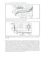
The DIN EN 206-1 [1] introduces mechanism-related exposure classes which
describe and account for environmental influences which are not directly taken
into account as loads for constructional measurement (Figure 2.74). From a
technological point of view, durability is determined by minimum concrete
composition requirements (water/cement ratio, cement content). The design

concept was derived from current knowledge of deterioration mechanisms and
correlations between exposure and resistance. This simple approach does, how-
ever, have the major disadvantage that the application of new materials and
concrete types for which there are as yet no empirical values is limited. Fur-
thermore, it is not possible to evaluate existing structures whose composition
is not known. Chronological changes in resistance to a different behavior com-
pared with the original exposure are also not recorded. A durability prognosis
of a concrete structure requires that the expected environmental conditions
to which the structure will be exposed can be reasonably reliably predicted.
The causes and correlations which lead to damage must be clearly recognized
and understand. Knowledge of damage mechanisms and the complex inter-
actions of external influences, transport and degradation process is necessary
for forecasting durability and serviceable life (Figure 2.74).
effect
intensity
chemical
attack
carbonation
process
chloride
penetration
Environmental Impact (classification of EN 206-1)
temperature and moisture
㩳
transport and/or reaction parameters
Climatic Conditions
frost attack with/
without de-icing agent
Degradation Process
Performance Concept

Incubation Time
limit
Serviceable Time
damage
criterion
Damage
reinforcement corrosion concrete corrosion
Fig. 2.74. Schematic diagram - Interaction of climate, environmental attack and
damage process - basis for the perfomance concept
94 2 Damage-Oriented Actions and Environmental Impact
(a) (b)
(c)
Fig. 2.75. Reinforcement corrosion (above): (a) due to the influence of chloride (b)
due to carbonation [400]; Concrete corrosion (below): (c) combined attack - AAR
intensified by alternating frost and thawing [529]
The damage process depends on the transport process. The efficiency of the
transport mechanisms is in turn dependent on moisture and/or temperature.
Moisture is necessary as a transport and reaction medium and the external
temperature works as a reaction accelerator. For example, the maximum car-
bonation speed occurs at humidities between 60% and 80% and the extent
of sulfate corrosion rises with sinking temperatures. In case of frost attack
the damage mechanisms only become active after the concrete texture is crit-
ically saturated through frost suction (transport mechanism). At the same
time, the ”real” environmental attack is a complex strain, the sum total of
several, sometimes simultaneous partial attacks which mutually influence one
another. For example, weathering with deep craters can lead to increased chlo-
ride penetration of the concrete by deicing salt or a deeper carbonation of the
concrete. This causes faster depassivation of the reinforcement, which causes
more rapid corrosion of the outer reinforcement (Figure 2.75 (b)). A further
example is the additional strain caused by temperature cycles, especially the

alternation of frost and thawing of the alkali-aggregate reaction (AAR). These
aid the development of the AAR by either leading to cracks in the concrete so
that it can be better penetrated by moisture and an AAR can be initiated, or
they lead to the expansion of existing AAR-related cracks (Figure 2.75 (c)).
2.4 Load-Independent Environmental Impact 95
Physical Action
thermal (e.g. freeze-thaw, freeze-deicing salt)
Chemical Action
dissolution (e.g. leaching, acid)
expansion (e.g. sulfates, alkali-aggregate reaction)
Concrete
Corrosion
Combined Action
e.g. alkali-aggregate reaction + freeze-thaw
Fig. 2.76. Attacks on concrete (in imitation of [872])
Figure 2.76 shows examples of physical and chemical environmental influ-
ences which cause concrete corrosion . The frost attack, the calcium leaching,
the sulfate attack and the alkali-aggregate reaction were processed as part of
SFB 398. It should be noted that in SFB 398 no practical examination of the
listed chemical attacks was performed and a summary of the practical exam-
inations in the literature can be found in Chapter 3. The laboratory tests are
accordingly also listed in Chapter 3. In addition, more detailed summaries of
the relevant aspects of durability in concrete structures can be found in e.g.
[770],[702].
2.4.2 Frost Attack (with and without Deicing Agents)
Authored by Ivanka Bevanda and Max J. Setzer
Frost and deicing salt attack are under the most detrimental environmen-
tal phenomena to be taken into account for durability design of concrete.
Frost attack with and without the presence of deicing salt is a dynamic ef-
fect that involves both a transport mechanism and a damage mechanism.

Setzer coined the term frost suction for the transport mechanism, and ex-
plained this phenomenon by surface physics described by the micro-ice-lens
model (see Subsection 3.1.2.2.3). During the freeze-thaw cycle, external water
is sucked inward by the action of the micro-ice-lens pump; the pore structure
becomes saturated. Only once the critical degree of saturation is exceeded
does ice expansion cause damage. Since there is not enough space in the con-
crete microstructure for lateral yield, critical internal stresses build up during
the process of ice formation, and then abate again as micro-cracks form. The
result of this is internal and/or external damage to the concrete structure.
External damage known as scaling (Figure 2.77) can be recognized as
(1) sandy decay and (2) local scaling of the hardened cement paste, and
in the case of aggregate-related damage as (3) popouts and (4) D-cracking.
96 2 Damage-Oriented Actions and Environmental Impact
Fig. 2.77. Surface of frost damaged concrete in situ [20]
External damage is the most frequently observed frost damage. It starts off
as an aesthetic fault, but then the surface destruction can lead to limitation
and loss of the function of the component, although structural stability is still
assured (e.g. in the case of airport taxiways). Internal damage is characterized
by microstructural damage arising from microcracks (Figure 2.78), which in-
fluence the mechanical and physical properties of the concrete structure, and
its structural integrity as a result. While both types of damage go hand-in-
hand with the critical degree of saturation and ice expansion, they still must
be treated as separate phenomena, since they appear not to be strictly re-
lated. In the case of external damage, dissolved substances (salts) add their
own damaging effect to the equation. This is an especially important factor
in the case of deicing salt attack, and is discussed at length in literature. New
findings, including those from SFB 398/ Project A11, show that even the in-
fluence of commonly ignored salt concentrations increases weathering in what
is regarded as ”pure” frost attack.
References in literature and our own investigations [21] show how diverse

the possible variations of alternating frost and deicing salt stressing of con-
crete components can be. One actual overview is given in the progress report
DAfStb
3
[737]. The progression of damage following pure frost attack was also
investigated under real climatic conditions (in situ) and under laboratory con-
ditions in SFB 398/ Project A11. The essential results and their significance
are summarized below.
2.4.2.1 The ”Frost Environment”: External Factors and Frost
Attack
Details on the composition and properties of the tested concretes are given
in [119],[120]. In order to emulate the conditions as realistically as possible,
the field samples were sealed and insulated on the sides, since moisture and
3
German Committee for Reinforced Concrete.
2.4 Load-Independent Environmental Impact 97
0,125
mm
Fig. 2.78. Microcracking of cement paste(left); ESEM image of frost damaged
concrete (right) [20]
Fig. 2.79. Field exposure (left); Modified multi-ring electrode (right)
heat transport through components is typically one-dimensional in real appli-
cations. A side overlapping edge for catching rainwater was attached onto the
test surfaces Figure 2.79. This way, a persistent water layer was simulated. In
real situations, this type of frost attack typically occurs on horizontal com-
ponents directly exposed to weathering, which are classified as exposure class
XF3 according to DIN EN 206-1 (frost attack without deicing salt, high water
saturation) [1]. Under the climatic conditions, there were alternating periods
of wetness and dryness, i.e. periods with dynamic moisture entry and redis-
tribution inside the specimen.

Climatically induced humidity and temperature stressing of the component
is the most important factor to consider when investigating frost damage. As
such, it was decided to obtain information on the changes in moisture con-
tent and concrete temperature using a modified multi-ring electrode
4
(MRE)
Figure 2.79. The modified MRE is a humidity/temperature sensor. Detailed
information on its construction and function are given in [660],[762].
4
Humidity sensor with integrated thermometers, pursuant to the Aachen patent.
98 2 Damage-Oriented Actions and Environmental Impact
5,0
5,5
6,0
6,5
7,0
7,5
8,0
8,5
9,0
3,40E-03 3,50E-03 3,60E-03 3,70E-03 3,80E-03
1/T [K
-1
]
ln (R)
0.7cm 8.11-10.11
0.7cm 10.11
0.7cm 11.11
0.7cm 15.11
0.7cm 16.11

3.4cm 10.11-16.11
T >0
o
CT <0
o
C
moisture
pentetration
drying
b = 4271
R
2
= 0.97
b = 4167
R
2
= 0.91
b = 2048
R
2
= 0.95
5,0
5,5
6,0
6,5
7,0
7,5
8,0
8,5
9,0

3,40E-03 3,50E-03 3,60E-03 3,70E-03 3,80E-03
1/T [K
-1
]
ln (R)
0.7 cm 10.11
0.7 cm 15.11
0.7 cm 18.11
T >0
o
C
T <0
o
C
Fig. 2.80. Effects at specific depths of water penetration, logarithm of resistance as
a function of reciprocal ground temperature (left); Dependence of Arrhenius factor
b on moisture content (right)
The resistance of concrete is dependent on both temperature and humid-
ity. Therfore, humidity changes and distribution can be derived from the
resistances measured if the temperature effect is taken into account. The
temperature dependence follows an Arrhenius equation
5
.TheArrhenius
factor b required for temperature compensation can be determined by taking
the logarithm of the exponential correlation between the reciprocal ground
temperature and the resistance with linear regression. What we find most
commonly in literature is that this temperature compensation is done by us-
ing a constant Arrhenius factor b. Our own tests confirmed the situation
found in [165],[701] namely that the activation energy depends on both tem-
perature and less pronounced on moisture content (Figure 2.80, right). In

order to determine the resistances precisely, the two influences should be de-
coupled, and the moisture and temperature-dependence of the Arrhenius
factor clearly defined. The dependency on moisture content can be given only
in approximation. Therefore, moisture measurement is limited to a qualitative
or semi-quantitative level. Even if the temperature dependency of resistance
could be evaluated only in a fair approximation of moisture content its results
allowed a clear definition of the point when ice formation sets in since here the
resistance increases at the same moisture content disproportionately, since the
ice basically acts as an insulator. A new, automatic data analysis system was
developed for analyzing the phase change from water to ice. That way, the
strong dependency of resistance on temperature was used in the data analysis
to analyze the number of phase changes, or the number of frost periods. The
data analysis system was verified by experimental laboratory events.
5
R
i
= R
o
∗ e
b

1
T
o
−
1
T
i

;R

i,o
- electrical resistance at temperature T
i,o
.
2.4 Load-Independent Environmental Impact 99
-20
-15
-10
-5
0
5
10
15
20
8.11 10.11 12.11 14.11 16.11 18.11 20.11 22.11 24.11 26.11 28.11
Days
Temperature [°C]
0
1
2
Percipitation [l/m²]
percipitation
air temperature
Fig. 2.81. Air temperature and rainfall; field station Meißen, local weather station,
11/08/05-11/28/05
An online monitoring system allowed continual recording. Under the ex-
isting exposure conditions the humidity readings and concrete quality were
not strictly correlated. Additionally, the strong dependence of the resistance
on temperature allowed only semi-quantitative conclusions on the moisture
content. However, by analyzing the relative change in humidity distribution

in the exposed concrete specimens in correlation with rainfall events, our tests
also confirmed the findings of [701] who studied the moisture penetration into
concrete under natural weathering conditions above freezing point. Schiegg
defines two types of incidents, depending on effects at specific times and ef-
fects at specific depths: small incidents (transport zone <20 mm, time of effect
over a number of days) and large incidents (transport zone >40 mm, long-
term effect over several months, moisture penetration occurring in multiple
phases).
The temperature and humidity-dependence of resistance can be seen clearly
in Figure 2.80. This partially shows the moisture penetration to depth level 3.4
cm into a specimen directly after field exposure (Field Station Meißen, East
Germany). Following Arrhenius equation the logarithm of resistance is pre-
sented as a function of the reciprocal ground temperature. On November 10, we
see that the resistance at a depth of 0.7 cm drops, since the first moisture pen-
etration occurred at that time. This also correlates with the recorded rainfall
event on that day (Figure 2.81). After that, there was a dry-out until Novem-
ber 15. Then, on November 15, a freeze-thaw cycle was recorded, but still no ice
formation process had taken place yet. While the resistance rises as tempera-
ture drops, it does so in linear fashion, and not in jumps as it characteristically
does right at the water-to-ice phase change (see Figure 2.82). On November 15,
there was further moisture penetration, which again resulted in a drop in resis-
tance. In the same period, there was no change in moisture content recorded
100 2 Damage-Oriented Actions and Environmental Impact
-5
-4
-3
-2
-1
0
1

2
3
4
5
4:48 AM 9:36 AM 2:24 PM 7:12 PM
Time [-]
Temperature [°C]
air temperature
1.7 cm
3.4 cm
6.6 cm
5,0
5,5
6,0
6,5
7,0
7,5
8,0
8,5
9,0
3,45E-03 3,55E-03 3,65E-03 3,75E-03 3,85E-03
1/T [K
-1
]
ln (R)
0.7 cm
1.7 cm
6.6 cm
T >0
o

CT <0
o
C
freeze thaw
cycles
frost suction
Fig. 2.82. Freeze-thaw cycle illustrated by example (left); Temperature curve during
thaw phase on November 26 (right)
at 3.4 cm depth, and the change in resistance is attributed to temperature
alone. The temperature-dependence of resistance can be compensated for us-
ing the Arrhenius equation. Greater moisture penetration into the specimen
interiors occurred in both winters before and/or at the beginning of the ”frost
period”. The concrete surface zone is essentially saturated before the actual
freezing phase (see Figure 2.80). Moisture absorption inside the specimens af-
ter a freeze-thaw cycle at the beginning of the ”cold period” can be attributed to
frost suction according to the micro-ice-lens model. Figure 2.82 shows an exam-
ple illustrating the change in moisture content after two successive freeze-thaw
cycles (Nov. 24/25 and Nov. 25/26). Resistance at all depth levels increases with
a jump when the temperature drops below the ”0
o
C transition”. Field and lab-
oratory results show that ice formation sets in at about -0.5
o
C. The resistance
curve also shows that the water continually freezes as temperature drops. After
the thaw process on November 26, the resistance at depth levels 0.7 and 1.7 cm
drops back down to the original value. At depth level 6.6 cm, on the other hand,
the resistance drops as it would for an increase in moisture content. A detailed
description of frost suction and the micro-ice-lens model is discussed in (see
Subsection 3.1.2.2.3). Here, it is of relevance that the frost pump is activated

during the thaw phase, with a penetrating melting front. External water can be
sucked inward together with this penetrating melting front. The temperature
curve shown in Figure 2.82 (right) shows the penetrating melting front at each
point in time.
The change in resistance in the winter phase reveals the following: (1)
the moisture penetration into the specimen can be attributed to individual
events at the beginning of the frost phase and (2) has a long-term action of
several months. This is illustrated by the example given for depth level 6.6 cm
(specimen core) in Figure 2.83. The most moisture penetration took place up
2.4 Load-Independent Environmental Impact 101
5,0
5,5
6,0
6,5
7,0
7,5
8,0
8,5
9,0
3,40E-03 3,50E-03 3,60E-03 3,70E-03 3,80E-03
1/T [K
-1
]
ln (R)
6.6 cm 11.11.
6.6 cm 26.11.
6.6 cm 02.12.
6.6 cm 20.02.
6.6 cm 22.03.
T >0

o
CT <0
o
C
Fig. 2.83. Exemplary illustration of the change in resistance at depth level 6.6 cm
in the winter of 05/06; field station Meißen
until November 30. In the phase after that, up until February 20, no change
in moisture content at this depth was recorded. From the end of February
06, it can be seen that the specimens started drying out. A diagram of the
resistance on March 22 is shown as an example. The moisture content at this
time practically matches the initial moisture content.
In the analysis of the data, a process is counted as a freeze or thaw phase
according to a combination of criteria - predefined minimum temperature and
signal drop - which in turn seems to depend on moisture content or ice for-
mation. The intensity of the frost attack distinguishes itself the most by the
minimum temperature and number of freeze-thaw cycles. Also, the damage is
increased by high cooling rates. Accordingly, the developed data analysis sys-
tem analyzes each freeze event individually and delivers the following data for
each depth level: minimum temperature, maximum and averaged cooling and
thawing rates, and time and duration of the individual phase changes. The rel-
evant data for the winter of 05/06 and 06/07 are summarized in Table 2.14.
Figure 2.84 shows the frequency of freeze-thaw cycles depending on mini-
mum temperature (left) and maximum cooling and thawing rates (right) for
measuring point 0.7 cm over the exposure period. Measuring point 0.7 cm is
especially of interest in connection with the observed surface damage to the
exposed concretes, which we shall discuss later. There is a difference between
the individual winters regarding the number of cycles and the minimum tem-
peratures (see Table 2.14). Nevertheless, the greatest number of freeze-thaw
events in both winter periods happened in the temperature range between -2
and -10

o
C. Between the individual specimens, there is no significant differ-
ence in the number of freeze-thaw cycles, the deviation being only 1 ftc. As
expected, the number of ftc drops in proportion to the depth level. In the
winter of 05/06, there were 40 ftc recorded at a depth of 0.7 cm, 39 at 1.7 and