Lifetime-Oriented Structural Design Concepts- P19 potx

498 4 Methodological Implementation
u
[
mm
]
F
[
kN
]
0.3
5
0.30.250.20.150.10.050
350
300
250
200
150
100
50
0
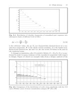
Fig. 4.94. Numerical investigation of crack propagation of an anchor pull-out test:
Load-displacement curve
displacement reaches u
z
≈ 0.21 [mm] the carck propagation nearly stops due
to the fact that most of the load is carried by the area of counter pressure.
This is evident from Figure(4.93,right) that shows the strongly increased value
of the stress component σ
33
at the counter pressure support. On the contrary
in the beginning of the cracking process (figure(4.93,left)) there is nearly no

compression at the area of counter pressure because of the load carrying of the
concrete in the vicinity of the anchor plate. When the displacement reaches
u
z
≈ 0.21 [mm], the load is primarily induced to the counter pressure sup-
ports by the nearly fully separated upper part of the concrete structure. This
bearing behaviour of the system is primarly characterized by the position of
the crack surface that is running underneath the pressure supports. In the
case that the crack reaches the upper surface of the concrete structure being
in front of the supports, there is going to be a structural softening of the
concrete block. This interpretation is similiary to the one in [301] where a
similiar numerical test is performed. As can be further deduced from Figure
4.93 there is a high compression atop of the anchor plate, which would also
lead to compression failure of concrete. This does not occur here, because this
analysis only takes failure of concrete in tension into account.
4.2.10 Substructuring and Model Reduction of Partially Damaged
Structures
Authored by Christian Rickelt and Stefanie Reese
The objective of this section is to present an efficient strategy to cope
with demanding dynamical simulations of complex structures. We are in par-
ticular interested in long term calculations like life cycle investigations. Our
4.2 Numerical Methods 499
ansatz emanates from the idea that a structure only comprises locally dis-
tributed damaged zones. The proposed method is an evolution of the classical
Craig-Bampton approach to partially damaged problems and incorporates
an advantageous decomposition of the entire structure into linear and non-
linear segments. The former are reduced by model reduction techniques. In
the nonlinear components the deterioration of the material is simulated by
a continuum damage model for ductile damage phenomena of metals. This
material model is included into a new solid beam finite element formulation

Q1SPb based on reduced integration with hourglass stabilisation. The section
closes with an example to validate the proposed strategy and to determine the
approximation error caused by the model reduction of the linear components.
4.2.10.1 Motivation and Overview
The importance of simulation tools for the design and lifetime estimation
of complex structures increases noticeably. Highly demanding tasks and re-
quirements on the accuracy of numerical computations necessitate powerful
simulation techniques and more elaborate models. Since in general these mod-
els cannot be solved analytically the underlying ordinary or partial differential
equations are often discretised and solved by the finite element method.
Dynamic problems require beside the spatial discretisation as well a dis-
cretisation in time. This can be accomplished by implicit or explicit time
integration schemes. While the former lead to large, sparse equation systems,
whose solution is memory and time consuming, the disadvantage of the ex-
plicit methods is that they are only conditionally stable. Accordingly its time
step size is limited by a critical time step. As a consequence the latter schemes
are not suitable for long-term computations.
Strategies to solve such complex long-term calculation numerically efficient
have been a topic of research in the field of engineering technologies and math-
ematics. More related to the former one are the condensation methods and the
staggered schemes. The domain decomposition methods are mostly researched
in mathematics while the model reduction techniques are established in both
communities.
The idea of model reduction is to transform the large equation system
into a small, dynamically equivalent substitute model. Powerful model reduc-
tion methods exist for the solution of linear and weakly nonlinear systems.
Highly nonlinear problems like the evolution of damage cannot be solved. [761]
and [808] employ nonlinear model reduction techniques to reduce geometri-
cally nonlinear problems and fluid-structure interactions, respectively. For an
overview of model reduction methods in general refer to the publications of

[111, 761, 49, 50, 651, 288, 76, 51, 451, 287, 236, 583, 485, 813].
Linear model reduction methods can be classified into three different
groups: the singular value decomposition (SVD)-based methods, the Krylov-
based methods and the condensation methods. Out of the group of SVD-
based model reduction two well-known methods are the Modal Reduction
500 4 Methodological Implementation
(MODRED) (see the standard text books [195, 203]) and the Proper Orthog-
onal Decomposition (POD) (see [121, 384, 755]). Two important members of
the Krylov-based methods are the Load-Dependent Ritz Vectors (LDRV)
(see [328, 203, 585]) as well as the Pad
´
e-Via-Lanczos algorithm (PVL).
In this publication a symmetric version for undamped second order systems,
called symmPVL, is used (see e.g. [288, 76]).
The above mentioned group of condensation methods comprise model re-
duction methods which condense the inner degrees-of-freedom (dofs) and con-
serve the physical interface dofs. This idea can be structured into static as well
as dynamic condensation methods. According to [620] the latter yield exactly
reduced dynamical systems which even for linear problems result in nonlinear
functions which depend on the frequency. Hence they are not numerically effi-
cient. In contrast the static condensation of [333] is suitable to only a limited
extent for the model reduction of linear dynamic systems. Corresponding to
the text book of [651] component mode synthesis techniques (CMS techniques)
establish a significant extension of Guyan’s reduction to methods with hy-
brid transformation matrices. Initialised by the classical papers of [401] and
[216] (see also the review article of [215]), CMS techniques with fixed inter-
faces have been developed within the scope of reduction methods for large
structural dynamic models and the design of single dynamical components
of challenging structures. These methods are based on the superposition of
different contribution of the deformations. Hence they are only valid for lin-

ear problems. For further information on CMS techniques see the overview
publications of [217, 206, 498, 722, 511].
Alternatively the objective of staggered algorithms (see for example [548])
is to solve multi-field or dynamic problems which are discretised by different
time integration schemes (implicit/explicit) and varying time step lengths
(subcycling) within each subdomain (see the classical papers of [108] and
[107]). An interesting approach of an explicit-implicit multi time step method
for nonlinear structural dynamics which prescribes the continuity of velocities
at the interface and uses a dual Schur formulation has been published by
[323]. [274] and [275] extend this ansatz successively to nonmatching meshes
and linear as well as nonlinear model reduction techniques.
The primary interest of domain decomposition methods, grouped into over-
lapping (”Schwarz methods”) and non-overlapping (”iterative substructur-
ing methods”) methods, is the development of highly efficient parallelised
iterative solution techniques. These usually result in conjugate gradient
schemes. The latter are subdivided into the Neumann-Neumann-(Bal-
anced Domain Decomposition (BDD), [515]), Dirichlet-Neumann-and
Dirichlet-Dirichlet-Algorithm (Finite Element Tearing and Interconnect-
ing Method (FETI), [273]). Most of the publications deal with linear problems.
Applications to geometrically nonlinear problems can be found in the papers
of [218] and [272].
4.2 Numerical Methods 501
Structural Dynamics
Modelling (FEM)
Linear Components Nonlinear Components
Model Reduction
Substructure
Technique
Damage
Modelling

Fig. 4.95. Concept for the efficient simulation of dynamic, partially damaged struc-
tures by means of model reduction and substructuring
4.2.10.2 Concept
In this section an efficient strategy for dynamic long-term simulations of com-
plex structures with local nonlinearities by means of the finite element method
is presented. Our approach emanates from the idea that engineering structures
are usually designed in such a way that most components of a structure be-
have linearly elastically and under the assumption of small deformations. Thus
undesired effects such as the evolution of damage or possibly occurring large
deformations are localised in small parts of a structure.
This ansatz, depicted in Figure 4.95, enables to decompose any discretised
structure strictly into its linear and nonlinear components. In the latter the
evolution of ductile damage of metals is considered. The damage model is
based on the void growth model of [691, 690]. Further we assume that the
evolution of damage is only influenced indirectly by the dominating linear
subsystems. Hence, to increase the efficiency of the strategy, the latter are re-
duced by model reduction methods in conjunction with the Craig-Bampton
method – one of the widely used CMS substructure techniques. Beside the
common Modal Reduction, linear model reduction methods of superior accu-
racy – the Pad
´
e-Via-Lanczos algorithm (PVL), the Load-Dependent Ritz
Vectors (LDRV) and the Proper Orthogonal Decomposition (POD) – are em-
ployed. Finally the substructuring of the total structure into reduced lin-
ear and nonlinear components is exploited. Instead of solving a large mono-
lithic equation system the system response of the redundant interfaces of the
components is computed. Subsequently the inner dofs of all components are
calculated.
One advantage of the presented concept rests upon the beneficial combi-
nation of well-known and robust linear model reduction methods, the CMS

502 4 Methodological Implementation
technique, the material as well as the efficient element formulation. Another
important aspect is the numerical implementation. For this purpose the math-
ematical development environment Matlab and the finite element program
Feap are linked by the interface Feapmex
1
.
4.2.10.3 Derivation of a Substructure Technique for Nonlinear
Dynamics
In this section the Craig-Bampton method is summarised. Afterwards the
linear model reduction methods and the employed substructure technique are
discussed.
4.2.10.3.1 Craig-Bampton Method
The concept of CMS techniques has been developed [401] and later rewritten
and simplified by [216] to analyse complex structural systems decomposed
into interconnected components with fixed interfaces. The Craig-Bampton
method superposes two different fractions of the motion: the static or con-
straint modes Ψ
ic
of the matrix Ψ
T
:=

Ψ
T
ic
I
T
cc


are defined as the static
deformation of a structure when a unit displacement is applied to one in-
terface dof while the remaining interface dofs are restrained. The matrix I
cc
herein is an identity matrix of dimension c × c. The indices i and c indicate
the inner and the interface dofs, respectively. The second fraction are the k
(k  i) remaining inner dynamical or so-called normal modes φ
j
,j=1, ,k
of the fixed subsystem s. They are stored column by column into the matrix
Φ
r
:=
⎡
⎢
⎣
φ
1
, ,φ
k
O
ck
⎤
⎥
⎦
=
⎡
⎢
⎣
Φ

ik
O
ck
⎤
⎥
⎦
. (4.243)
The matrix O
ck
is a zero matrix of dimension c × k. Usually the modes Φ
ik
are represented by eigenvectors. In this contribution the LDRV-, POD- or
symmPVL-vectors of alternative model reduction methods of superior accu-
racy, as presented in section 4.2.10.3.2, are utilised. With these modes the
physical coordinates u can be transformed by the relation
⎡
⎢
⎣
u
i
u
c
⎤
⎥
⎦

 
u
(s)
=

⎡
⎢
⎣
Φ
ik
Ψ
ic
O
ck
I
cc
⎤
⎥
⎦

 
V
(s)
CB
⎡
⎢
⎣
q
k
q
c
⎤
⎥
⎦


 
q
(s)
(4.244)
into generalised coordinates q. V
CB
symbolises the well-known Craig-Bamp-
ton transformation matrix of one single component s. Transforming with
1
For further information see the following homepage:
www.cims.nyu.edu/ dbindel/feapmex/feapmex/doc/feapmex.html
4.2 Numerical Methods 503
the relation (4.244) the linear equation of motion of one component s by an
orthogonal projection
V
(s)
CB
T
M
(s)
V
(s)
CB
  
M
(s)
rr
¨
q
(s)

(t)+V
(s)
CB
T
K
(s)
V
(s)
CB
  
K
(s)
rr
q
(s)
(t)=V
(s)
CB
T
b
(s)
  
b
(s)
r
f(t)
(s)
(4.245)
leads for linear undamped systems to a component of smaller dimension in
which the interface dofs u

c
= q
c
are conserved in physical coordinates. In the
latter equation M, K, b and f(t) are the mass matrix, the stiffness matrix, the
load distribution and the loading function. The index r denotes the dimension
of the reduced component.
4.2.10.3.2 Model Reduction of Linear Dynamic Structures
Besides our objective to save computational effort by decomposing a structure
into its linear and non-linear parts the linear substructures are approximated
by dynamically equivalent subsystems. Within the Craig-Bampton method
the fixed interface normal modes of each component are defined as a reduced
set of modes by restraining all boundary dofs. These modes Φ
ik
form part of
the Craig-Bampton transformation matrix V
CB
(see section 4.2.10.3.1). In
this contribution we will derive the model reduction of linear dynamic systems
within a general framework. For simplicity we leave out the superscript s.We
start from the ansatz
u
i
= Φ
ik
q
k
(4.246)
in which u
i

is the displacement vector, q
k
is the vector of the reduced system
and Φ
ik
is a rectangular projection matrix of the dimension (i × k). This
approach is inserted into the linear equation of motion
K
ii
u
i
+ M
ii
¨
u
i
= b
i
f(t) . (4.247)
This leads to a set of linear equations of reduced dimension
(Φ
ik
)
T
K
ii
Φ
ik
  
K

kk
q +(Φ
ik
)
T
M
ii
Φ
ik
  
M
kk
¨
q =(Φ
ik
)
T
b
i
  
b
k
f(t) . (4.248)
In the following four different projection-based model reduction methods are
summarised. These methods are the Modal Reduction, the Proper Orthogonal
Decomposition (POD), a symmetric Pad
´
e-Via-Lanczos algorithm (symm-
PVL) and the Load-Dependent Ritz Vectors (LDRV).
4.2.10.3.2.1 Modal Reduction

Modal Reduction, also known as Modal Truncation, is the most simple
and popular model reduction method. The idea is to solve a subset of the
504 4 Methodological Implementation
generalised eigenvalue problem in which Φ
ik
=[φ
1
, φ
2
, ··· , φ
k
] is the reduced
modal matrix and Λ
kk
=diag

ω
2
1
,ω
2
2
, ···,ω
2
k

is the reduced eigenvalue
matrix. After a mass normalisation
(Φ
ik

)
T
K
ii
Φ
ik
= Λ
kk
, (Φ
ik
)
T
M
ii
Φ
ik
= I
kk
(4.249)
a reduced decoupled differential equation system is obtained:
Λ
kk
q
k
+ I
kk
¨
q
k
= b

k
f(t) . (4.250)
4.2.10.3.2.2 Proper Orthogonal Decomposition
A second possibility is the POD method. This method is also known as
empirical eigenvectors, Karhunen-Lo
`
eve expansion, principle component
analysis, empirical orthogonal eigenvectors, etc. An overview of nomenclatures
used in the literature and areas of application are given e.g. in [121].
The mathematical basis for the POD method is the spectral theory of
compact, selfadjoint operators which is explained e.g. in the standard text
book of [384]. One problem of this ansatz is that even for small systems
the eigenvectors of a large spatial covariance matrix have to be calculated.
One approach to lower the computational costs is known as the “method of
snapshots” ([755]). In this case each POD basis vector
φ
l
=
m

j=1
β
j
w
j
l =1, ,k (4.251)
is generated out of m uncorrelated zero-mean “snapshots” w
j
. In the latter
equation w

j
= u
j
−
¯
u describes the deviation of the “snapshot” u
j
from their
temporal mean
¯
u. β
j
are unknown coefficients which have to be determined.
After some derivations and using the assumption that the investigated pro-
cess is ergodic (see e.g. [536, 384]) only a reduced eigenvalue problem of di-
mension m ×m
1
m
W
T
W β
l
= λ
l
β
l
with W =[w
1
, ··· , w
m

] , (4.252)
in which W contains the m zero-mean “snapshots” has to be solved. The k
basis vectors of the POD
φ
l
= W β
l
, (4.253)
corresponding to the eigenvalues λ
1
>λ
2
> ··· >λ
l
> ··· >λ
k
,resultfrom
a linear combination of the zero-mean “snapshots”.
4.2.10.3.2.3 Pad´e-Via-Lanczos Algorithm
The Pad
´
e-Via-Lanczos algorithm and the Dual Rational Arnoldi
method belong to the Krylov-based model reduction methods. This
4.2 Numerical Methods 505
system-theoretical approach for first order differential equations can also
be applied to second order systems. A differential-algebraic equation system
K
ii
u
i

(t)+M
ii
¨
u
i
(t)=b
i
f(t) y(t)=c
i
u
i
(t) (4.254)
is converted by the Laplace transformation to the transfer function
H(s)=c
i
[s
2
M
ii
+ K
ii
]
−1
b
i
(4.255)
Here the equations are given for a single input single output (SISO) systems.
The measurement vector c
i
of the dimension (1 × i) relates the displacement

vector u
i
(t) to the measured output y(t) of the system.
The transfer function (4.255) is re-written and expanded around an expan-
sion point σ
2
into a power series (Laurent or Taylor series)
H(s)=c
i
[(K
ii
− σ
2
M
ii
)+(σ
2
+ s
2
) M
ii
]
−1
b
i
= c
i
[I
ii
− (K

ii
− σ
2
M
ii
)
−1
(−σ
2
− s
2
)M
ii
]
−1
(K
ii
− σ
2
M
ii
)
−1
b
i
=
∞

j=0
μ

j
(−σ
2
− s
2
)
j
(4.256)
The coefficients μ
j
= c
i
((K
ii
−σ
2
M
ii
)
−1
M
ii
)
j
(K
ii
−σ
2
M
ii

)
−1
b
i
are termed
“moments”. Thus the method is also called “moment matching” in the
literature.
An important observation for the Pad
´
e approximation presents the fact
that the moments can be computed in a numerically stable fashion by Krylov
subspace methods like the Lanczos or the Arnoldi method.
For the special case c
T
i
= b
i
and symmetric, positive definite matrices
M
ii
and K
ii
[290] show that the reduced systems are stable. According to
[486] for mechanical problems purely imaginary expansion points σ = jω
c
are
chosen (ω
c
is the angular frequency in the centre of the interesting frequency
range). Employing a Cholesky decomposition K

ii
− σ
2
M
ii
= N
ii
N
T
ii
and
the relations r
i
= N
−1
ii
b and G
ii
= N
−1
ii
M
ii
N
−T
ii
the transfer function is
transformed into
H(s)=r
T

i
[I
ii
+ G
ii
(σ
2
+ s
2
)]
−1
r
i
. (4.257)
Using the Lanczos algorithm the matrix G
ii
is approximated by a tridiago-
nalised matrix T
kk
of the dimension k × k. In the time domain the reduced
system results in
T
kk
¨
q
k
(t)+[I
kk
+ σ
2

T
kk
]q
k
(t)=r
k
f(t)
y(t)=r
T
k
q
k
(t)
(4.258)
506 4 Methodological Implementation
The reduced vector r
k
=(Φ
ik
)
T
r
i
is computed according to the projection
(4.248). The proposed algorithm for symmetric positive definite system is
termed in the following symmPVL.
4.2.10.3.2.4 Load-Dependent Ritz Vectors
The method of Load-Dependent Ritz Vectors (LDRV) is an approach of
structural dynamics. In the special case that the matrices M
ii

and K
ii
are
symmetric positive definite matrices, the expansion point is zero (σ = 0), the
basis vectors are mass normalised and the input and measuring vectors are
identical (c
T
i
= b
i
) this algorithm is similar to the SyPVL algorithm proposed
by [289].
The LDRV are based on the Lanczos algorithm together with a special
start vector. Here the static deflection is used as the first Ritz vector so that
all following Ritz vectors may be regarded as the balancing of this initial
deflection (see [851]). The advantage of this method is that no eigenvalue
problem has to be solved.
According to [585] the method delivers the following reduced coupled dif-
ferential equation system:
T
kk
¨
q
k
+ I
kk
q
k
= {β
1

, 0, ··· , 0}
T
f(t) (4.259)
Herein the stiffness matrix and the mass matrix are degenerated to an iden-
tity matrix I
kk
and a tridiagonal matrix T
kk
in generalised coordinates,
respectively. If we assume that the load distribution on the structure is con-
stant during the simulation, the projected external load vector reduces to
b
k
= {β
1
, 0, ··· , 0}
T
f(t). The scalar value β
1
=

ϕ
T
1
M ϕ
1
is given by the
first not mass normalised Ritz vector ϕ
1
.

4.2.10.3.3 Substructuring in the Framework of Nonlinear Dynamics
The derivation is based, as displayed in Figure 4.96, on a decomposition of
the structure into two arbitrary components. Only with the assembly and the
solution of the equation system one of the two components is limited to a
reduced linear subsystem.
4.2.10.3.3.1 Discretisation and Linearisation
Starting point is the balance of linear momentum of a subsystem s in the
reference configuration
Div P
(s)
+ ρ
0
b
(s)
v
− ρ
0
¨
u
(s)
+ F
(s)
c
= 0 s =1, 2 . (4.260)
Herein is P
(s)
the first Piola-Kirchhoff stress tensor, b
(s)
v
the volume force

vector,
¨
u
(s)
the acceleration vector and ρ
0
the mass density in the reference
configuration. Additionally interface forces F
(s)
c
have to be introduced. These
internal forces only possess non-zero components at the redundant interfaces
Γ
(s)
c
. As constraints the equilibrium of the interface forces
4.2 Numerical Methods 507
Component (1) Component (2)
Interface no de
Internal node
Ω
(1)
0
Ω
(2)
0
Γ
(1)
c
Γ

(2)
c
Fig. 4.96. Decomposition of the structure into two components
F
(2)
c
− F
(1)
c
= 0 (4.261)
and the compatibility condition of the deformed configuration
g = x
(2)
c
− x
(1)
c
= 0 (4.262)
has to be fulfilled. x
(s)
c
= u
(s)
c
+ X
(s)
c
is the position vector of the deformed
configuration at the interface. It is composed of the displacement vector u
(s)

c
and the position vector of the undeformed reference configuration X
(s)
c
.
The interface forces may be replaced by the Lagrange-multipliers
λ
(1)
c
= λ
(2)
c
= λ
c
(4.263)
since the interface area is of identical size. In the field of contact simulations
λ
c
is named contact pressure. If equation (4.263) is inserted into the strong
forms (4.260) and (4.262) in accordance with [473, 856] each subsystem s can
be transformed into the weak form
g
1
(u
(s)
, λ)=
2

s=1



Ω
(s)
0
P
(s)
·Grad δu
(s)
dΩ
(s)
0
+

Ω
(s)
0
ρ
0
¨
u
(s)
·δu
(s)
dΩ
(s)
0
−

Ω
(s)

0
ρ
0
b
(s)
v
·δu
(s)
dΩ
(s)
0
−

Γ
(s)
T
¯
T
(s)
·δu
(s)
dΓ
(s)
T

+

Γ
c
λ ·(δu

(2)
− δu
(1)
) dΓ
c
=0
g
2
(u
(s)
, λ)=

Γ
c
(x
(2)
− x
(1)
) ·δλ dΓ
c
=0
(4.264)
508 4 Methodological Implementation
which refers to the initial configuration Ω
(s)
0
. The last integral in Equation
(4.264a) specifies the virtual work of the Lagrange multipliers λ at the
interface. Equation (4.264b) enforces the constraint condition in a weak sense.
δu

(s)
and δλ are the test functions of the independent variables u
(s)
and λ.
The external boundary of each component Γ
(s)
= Γ
(s)
u
∪Γ
(s)
T
∪Γ
(s)
c
consists of
the Dirichlet boundary Γ
(s)
u
,theNeumann boundary Γ
(s)
T
and the interface
boundary Γ
(s)
c
. The vector
¯
T
(s)

represents the external tensions.
Beside a spatial discretisation according to the isoparametric element con-
cept the constraints at the interface are fulfilled in a strong manner. Hence
the virtual work of the Lagrange multiplier at the interface (4.264a) and
the compatibility constraint (4.264b)

Γ
c
λ ·(δu
(2)
− δu
(1)
) dΓ
c
=
nn
c

i=1
Λ
i
(δu
(2)
i
− δu
(1)
i
)
=[δu
(1)

i
T
δu
(2)
i
T
]
⎡
⎢
⎣
−
d
C
(1)
T
d
C
(2)
T
⎤
⎥
⎦
T
Λ
= δu
Td
C
c
T
Λ


Γ
c
(x
(2)
− x
(1)
) ·δλ dΓ
c
=
nn
c

i=1
(u
(2)
i
− u
(1)
i
) δΛ
i
= δΛ
T
[−
d
C
(1) d
C
(2)

]u
= δΛ
T
d
C
c
u
= δΛ
T
d
G
c
(4.265)
are transformed into a summation over all interface nodes nn
c
.Theinterface
force Λ
i
= λ
i
·A
i
at node i is the product of the Lagrange multiplier λ
i
and
the corresponding area A
i
of node i. δu
(s)
i

and δΛ
i
are the test functions of
node i. Additionally the position vectors at the corresponding interface nodes
X
(1)
≡ X
(2)
are identical. As a result in Equation (4.265b) the difference
between the position vectors of the deformed configuration x
(s)
is replaced
by the the difference of the displacements u
(s)
.Thematrix
d
C reduces in the
discrete case to a Boolean allocation matrix. At this the index d indicates that
the interface constraints are fulfilled in a strong manner.
Finally incorporating any time integration like e.g. the Newmark method
we result in the fully discretised nonlinear equation system subjected to a
constraint:
4.2 Numerical Methods 509
R(u
n+1
)+M
¨
u
n+1
(u

n+1
)− P
ext
+
d
C
T
c
Λ
n+1
:=
G(u
n+1
)+
d
C
T
c
Λ
n+1
  
d
G
g
(u
n+1
,Λ
n+1
)
≈ 0

d
G
c
(u
n+1
)=0 .
(4.266)
n + 1 denotes the current time step which is omitted below. R(u)andP
ext
are the inner and the external force vectors, respectively.
d
G
g
(u
n+1
)and
d
G
c
(u
n+1
) are the residual vectors.
To solve Equation (4.266) by the Newton-Raphson method a consistent
linearisation with respect to the independent variables u and Λ leads to the
linearised and decoupled system
⎡
⎢
⎣
K
T eff

(u
m
)
d
C
T
c
d
C
c
O
⎤
⎥
⎦
⎡
⎢
⎣
Δu
m+1
ΔΛ
m+1
.
⎤
⎥
⎦
= −
⎡
⎢
⎣
G(u

m
)+
d
C
T
c
Λ
m
d
C
c
u
m
⎤
⎥
⎦
(4.267)
in matrix notation.
The indices eff and m denote that in the tangential stiffness matrix K
T eff
the time discretisation is already included as well as m signifies the number of
iterations. Both indices are omitted below in order to improve the readability.
4.2.10.3.3.2 Primal Assembly
The objective of this strategy is to solve partially reduced systems with
local nonlinearities such as material damage behaviour. Thus in the follow-
ing derivation the components (1) and (2) are regarded to be the nonlinear
subsystem (nl) and subsystem (2) the reduced, but linear subsystem (lin).
The ( )-symbol is used to indicate reduced components. The transforma-
tion of the reduced linear subsystem (2) results from the presented Craig-
Bampton transformation u

(2)
= V
(2)
CB
q
(2)
. The vectors u
(2)
and q
(2)
are the
physical and the generalised coordinates of the linear component (2).
In the following synthesis of the components, which is published by [217]
for linear systems, the interface forces are regarded as Lagrange multipli-
ers. At first the compatibility condition (4.266b) has to be transformed into
generalised coordinates
d
C
q
q = 0 (4.268)
and is split
d

C
dd
C
de

q
⎡

⎢
⎣
q
d
q
e
⎤
⎥
⎦
= 0 (4.269)
510 4 Methodological Implementation
into e coordinates which have to be kept and d coordinates which are deleted
or assembled.
The transformation of the not assembled generalised coordinates q to as-
sembled generalised coordinates p is carried out by the projection
⎡
⎢
⎣
q
d
q
e
⎤
⎥
⎦

 
q
=
⎡

⎢
⎣
−C
−1
dd
C
de
I
ee
⎤
⎥
⎦

 
R

q
e



p
.
(4.270)
The latter equation also holds in incremental form:
Δq = R Δp . (4.271)
Considering the two relations (4.269) and (4.270) the identity
d
C
q

R = O (4.272)
holds.
For the considered case of a nonlinear and a linear reduced subsystem with
physical interface dofs the relation (4.270) transforms to:
q =
⎡
⎢
⎢
⎢
⎢
⎢
⎣
q
(1) nl
e
q
(1) nl
d
q
(2) lin
e
q
(2) lin
e
⎤
⎥
⎥
⎥
⎥
⎥

⎦
=
⎡
⎢
⎢
⎢
⎢
⎢
⎣
u
(1) nl
i
u
(1) nl
c
q
(2) lin
k
u
(2) lin
c
⎤
⎥
⎥
⎥
⎥
⎥
⎦
=
⎡

⎢
⎢
⎢
⎢
⎢
⎣
IOO
OO I
OIO
OO I
⎤
⎥
⎥
⎥
⎥
⎥
⎦
⎡
⎢
⎢
⎣
u
(1) nl
i
q
(2) lin
k
u
c
⎤

⎥
⎥
⎦
. (4.273)
Substituting (4.273) in incremental form into the first equation of (4.267)
⎡
⎢
⎢
⎢
⎢
⎢
⎢
⎣
K
(1) nl
ii
K
(1) nl
ic
K
(1) nl
ci
K
(1) nl
cc

K
(2) lin
kk


K
(2) lin
kc

K
(2) lin
ck

K
(2) lin
cc
⎤
⎥
⎥
⎥
⎥
⎥
⎥
⎦
⎡
⎢
⎢
⎢
⎢
⎢
⎢
⎣
Δu
(1) nl
i

Δu
(1) nl
c
Δq
(2) lin
k
Δu
(2) lin
c
⎤
⎥
⎥
⎥
⎥
⎥
⎥
⎦
= −
⎡
⎢
⎢
⎢
⎢
⎢
⎢
⎣
G
(1) nl
i
G

(1) nl
c

G
(2) lin
k

G
(2) lin
c
⎤
⎥
⎥
⎥
⎥
⎥
⎥
⎦
+
d
C
T
q
Λ
m+1
(4.274)
which is further multiplied by R
T
, we arrive at the direct assembled global
system

⎡
⎢
⎢
⎣
K
(1) nl
ii
K
(1) nl
ic

K
(2) lin
kk

K
(2) lin
kc
K
(1) nl
ci

K
(2) lin
ck
K
(1) nl
cc
+


K
(2) lin
cc
⎤
⎥
⎥
⎦
⎡
⎢
⎢
⎣
Δu
(1) nl
i
Δq
(2) lin
k
Δu
c
⎤
⎥
⎥
⎦
= −
⎡
⎢
⎢
⎣
G
(1) nl

i

G
(2) lin
k
G
(1) nl
c
+

G
(2) lin
c
⎤
⎥
⎥
⎦
(4.275)
4.2 Numerical Methods 511
The iteration index m + 1 in Equation (4.274) is only applied to underline
that the latter equation depends on the current Lagrange multipliers.
4.2.10.3.3.3 Solution of the Decomposed Structure
The most common solution in the literature is the monolithic solution of
the overall equation system. In this work the existing decomposition of the
structure into large linear and small nonlinear components and the model
reduction of the linear subsystems is exploited to substitute the solution of
one monolithic equation system by the efficient solution of a number of small
equation systems. On the basis of Equation (4.273) the individual linear and
nonlinear components are transformed by means of static condensation into
the local Schur complement systems



K
(s) lin
cc
−

K
(s) lin
ck


K
(s) lin
kk

−1

K
(s) lin
kc


 
S
(s) lin
Δu
(s) lin
c
=


G
(s) lin
c
−

K
(s) lin
ck


K
(s) lin
kk

−1

G
(s) lin
k
  
G
(s) lin
+
d
C
(s)
q
T
Λ

(s)
(4.276)
and

K
(s)nl
cc
− K
(s)nl
ci

K
(s)nl
ii

−1
K
(s)nl
ic


 
S
(s)nl
Δu
(s)nl
c
= G
(s)nl
c

− K
(s)nl
ci

K
(s)nl
ii

−1
G
(s)nl
i
  
G
(s)nl
+
d
C
(s)
c
T
Λ
(s)
(4.277)
S
(s) lin
and S
(s)nl
represent the local Schur complements as well as G
(s) lin

and G
(s)nl
the modified residual vectors.
Accordingtotheprevious section the Lagrange multipliers cancel out
during the assembly process by means of direct elimination. As a result the
global Schur complement system
S
g
Δu
c
= G
g
(4.278)
is independent of the Lagrange multipliers. The global Schur complement
S
g
and the modified global residual G
g
are divided into its linear and nonlinear
components:
512 4 Methodological Implementation
S
g
= S
lin
g
+ S
nl
g
=

N
lin

s=1
(R
(s)
)
T
S
(s) lin
R
(s)
+
N
nl

s=1
(R
(s)
)
T
S
(s)nl
R
(s)
G
g
= G
lin
g

+ G
nl
g
=
N
nl

s=1
(R
(s)
)
T
G
(s) lin
+
N
nl

s=1
(R
(s)
)
T
G
(s)nl
(4.279)
R
(s)
represent rectangular Boolean submatrices of the global assembly ma-
trix R. They link the local interface dofs u

(s)
c
with the global interface u
c
.
The complete number of subsystems N = N
lin
+ N
nl
consists of N
lin
linear
components and N
nl
nonlinear components.
Finally, depending on the solution of the global Schur complement system
(4.278) the internal dofs
Δq
(s) lin
k
=


K
(s) lin
kk

−1



G
(s) lin
k
−

K
(s) lin
kc
Δu
(s) lin
c

Δu
(s)nl
k
=

K
(s)nl
ii

−1

G
(s)nl
i
− K
(s)nl
ic
Δu

(s)nl
c

(4.280)
are to be determined.
4.2.10.4 Example: M¨unster-Hiltruper Road Bridge
This example serves to validate the overall strategy. At first the solution of
the decomposed but unreduced structure is compared to a monolithic solution.
Subsequently the influence of the different employed model reduction methods
on the accuracy of the computation is investigated.
In this example the bar-like structure of an arched steel bridge is regarded.
Its geometry is based on the road bridge in M¨unster-Hiltrup (federal road
B54), which is one of the reference buildings of the Collaboratory Research
Centre 398. The dimensions, cross sections and parameters are chosen ac-
cording to existing mechanical drawings. In accordance with the proposed
strategy the structure is subdivided into linear and nonlinear components.
The former are additionally reduced to increase the numerical efficiency. The
results of the simulation are compared to the solution of a monolithic transient
analysis.
The road bridge, depicted in Figure 4.97, is l = 87.37 m long, b = 17.85 m
wide and h = 13.68 m high. In the nonlinear substructures we model the
evolution of material deterioration for ductile damage behaviour of metals.
For this purpose we extend the material model of Rousselier (see [691]).
Compare also [251] where an alternative approach has been chosen. The
material parameters read E = 210 000 N/mm
2
, ν =0.3, ρ
0
=7.85 kg/dm
3

,
σ
y0
= 400 N/mm
2
, H = 2100 N/mm
2
,D=2.0, σ
k
= 400 N/mm
2
,f
0
=0.01,
f
N
=0.25, ε
N
=0.2ands=0.4.
4.2 Numerical Methods 513
q
1
q
2
P
h
b
l
Load Function
t

1
t
2
t
3
X
1
X
2
X
3
Fig. 4.97. Discretised quarter of the bridge - geometry and loading
To simulate the deterioration within the hangers, a horizontal spatial force
of q
1
=2.2N/mm
2
is applied to the largest hanger. Additionally a vertical
force of q
2
=0.25 N/mm
2
and two single forces of P = 600 kN are loaded on
the cross girders of the girder and the cross girders of the arch, respectively.
The loading process is carried out linearly in t
1
=1.2 · 10
−1
s. After a constant
period of 1 · 10

−2
s the structure is completely unloaded. The loading function
is plotted in Figure 4.97.
The bridge structure is investigated for a symmetric loading case. As a
result only one quarter of the bridge is discretised. Besides the loading condi-
tions which result from the symmetric configuration the bridge is supported
vertically on l
bearing
=1.189 m long bearings at the ends of the girder.
The spatial discretisation of the bridge is accomplished by solid beam ele-
ments Q1SPb of the finite element family Q1SP. These eight node solid beam
elements are an extension of the solid shell element formulation of [666]. They
possess 2 × 2 Gauss points on their mid plane (perpendicular to the beam
axis). As a result Q1SPb elements are suitable to capture bending phenomena
of slender structures in a numerically efficient way with only one element over
the height. A further advantage of this finite element formulation is that any
inelastic material behaviour can be implemented without further kinematic
restrictions. These solid beam elements demonstrate their efficiency in the
paper of [667]. Therein they are used to simulate the behaviour of medical
stents made of shape memory alloys.
For an appropriate discretisation of the bridge some modifications are re-
quired. To reduce the numerical effort the cross sections of the arch, the
girder and the hanger have to be transformed into equivalent rectangular
cross sections. In Table 4.8 the corresponding cross sections and the associ-
ated material parameter are listed. Another simplification concerns the hanger
of the bridge: Since they hold only small-sized cross sections compared to the
514 4 Methodological Implementation
Table 4.8. Equivalent square sections and corresponding material parameters
Section Square Section Young’s Modulus Density
(b×h) [ mm × mm ] [N/mm

2
] [kg/dm
3
]
Girder (lin) 240 × 1400 205000 1.81
Arch (lin) 700 × 600 198000 1.88
Hanger (nl) 100 × 100 181000 7.46
A
B
C
Fig. 4.98. Exploded view of the bridge (complete system)
remaining bridge, they are approximated and connected to the structure by
(solid) beam elements.
The time integration of the example is carried out by the Newmark
method and a time step length of Δt = 10
−3
s.ThesamelengthΔt
POD
=Δt
is utilised in the precalculation step to collect the data sets for the POD
method. In this example a data basis composed of 400 data sets has shown to
be advantageous. A transient analysis is accomplished under the assumption
that large deformations and an accompanying evolution of damage only oc-
cur in the slender hangers. Hence the girders, the arches as well as the cross
girders are discretised by linear elastic Q1SPb solid beam elements, while the
damage model is only considered within the hangers and their junctions.
4.2 Numerical Methods 515
f
0,018
0,014

0,010
Fig. 4.99. Damage evolution in the largest two hangers at the end of the simulation
(initial damage f
0
=0.01)
This enables to decompose the discretised quarter of the bridge into its
linear and nonlinear components according to the proposed strategy. In this
example these are the linear girder, the linear arch as well as five nonlinear
hangers of the discretised quarter of the bridge. The single components of the
entire structure and the points of interest are visualised in Figure 4.98 by an
exploded view.
In point B (centre of the largest hanger) the system response of a nonlin-
ear subsystem is evaluated. Point C (upper junction of the largest hanger)
is the place of maximal damage evolution (cp. Figure 4.99). The maximal
deterioration at the end of the simulation is f
max
=2.73 · 10
−2
.
In the following investigation the dimension of the linear subsystems is re-
duced via the presented model reduction techniques. The solution is compared
to the system response of the unreduced structure. In the chosen discretisation
the arch and the girder consist of 2226 and 4898 inner dofs, respectively. There-
with the reduction of the linear subsystems from 1 up to 100 basis vectors cor-
responds to a reduction of the original size of the linear inner equation systems
from 0.02 % up to 4 %. The dimension of the Schur complement is 138 dofs.
In Figure 4.100 the system response concerning the largest examined
reduction basis of 100 basis vectors is regarded. Between the unreduced
and the partially reduced solution of the MODRED, the LDRV and the
516 4 Methodological Implementation

100 LDRV
100 symmPVL
100 POD 400
100 MODRED
Complete system
Time [s]
in point B [mm]
Displacement in X
2
− direction
1.210.80.60.40.2
1200
1000
800
600
400
200
Fig. 4.100. Displacement in X
2
-direction in point B and a reduction of the linear
subsystems to 100 basis vectors
LDRV
symmPVL
POD 400
MODRED
Number of basis vectors
in X
2
− directioninpointB[−]
Error in the displacement

100908070605040302010
10
+00
10
−01
10
−02
10
−03
Fig. 4.101. Mean relative displacement-based error 
u,Σ
in X
2
-direction in point B
and a reduction of the linear subsystems
symmPVL no difference is distinguishable. Solely the solution of the POD
exhibits a significant deviation to the unreduced solution. This result shows
the slight influence which has an exchange of the local element shape functions
towards a small number of unphysical global functions.
For a more detailed quantitative evaluation of the reduction error the mean
relative displacement-based error

u,Σ
=
1
N
N

i=1
min(

|u
A
(t
i
) − ¯u
A
(t
i
)|
(|¯u
A
(t
i
)|)
;1.0)
4.2 Numerical Methods 517
is defined. Herein N is the number of discrete time steps. The estimated
error over an interval of 1 up to 100 basis vectors is depicted in Figure 4.101.
Obviously all reduction basis exhibit quantitatively up to a size of 30 basis
vectors comparable reduction errors. Subsequently the LDRV, the symmPVL
and the POD reveal up to a basis of 50 or 60 basis vectors a reduction period
in which the model reduction errors do not improve or even increases with the
increasing dimension of the reduced components. Aside from Modal Reduction
it becomes evident that an increase of the number of basis vectors does not
automatically lead to a better approximation of the dynamical behaviour of
the reduced subsystems. The LDRV and the symmPVL, which both dispose
the Lanczos-Algorithm, show an almost identical reduction error.
For reduced subsystems with more than 60 basis vectors both methods
show a slightly larger reduction error than the Modal Reduction. The latter
yields in conjunction with the Craig-Bampton method the lowest reduction

error. In contrast the POD only captures the principle dynamic characteristics
of the systems. Higher modes do not induce an improvement of the accuracy.
As a consequence the method remains on an error level which has already
been reached with only 10 or 20 basis vectors.
The reason for the good performance of the Modal Reduction is based on
the fact that the reduced linear parts of this example are only slightly loaded.
Thus the main disadvantage of the Modal Reduction - to approximate exter-
nal loads inaccurate - has less influence on the result. Accordingly the Modal
Reduction yields for the reduction of unloaded subsystems, as proposed by
[313], accurate results. Additionally [111] mentions that the difference in the
reduction quality of reduced linear total systems between the Modal Reduc-
tion and reduction methods of higher accuracy (like the LDRV, symmPVL
or POD) is in the time domain of lower importance than in the frequency
domain. Finally the error level of the Craig-Bampton substructure tech-
nique and the reduction methods superpose each other. All these reasons lead
to results which differ from the model reduction of total systems. There the
minor accuracy of the Modal Reduction is not competitive to the other model
reduction methods.
Altogether the substructuring of complex systems into a number of smaller
components and the strong reduction of the dominating linear subsystems
results in a numerically efficient simulation strategy for partially damaged
systems. The additionally introduced reduction error is small.
4.2.11 Strategy for Polycyclic Loading of Soil
Authored by Andrzej Niemunis, Torsten Wichtmann
and Theodoros Triantafyllidis
In FE calculations of the accumulation of settlement due to high-cyclic
loading two different numerical strategies are combined. They are termed the
implicit and the explicit mode of operation.
518 4 Methodological Implementation
In the implicit mode each cycle is calculated with small increments

˙
σ(D)Δt.
The accumulation results as a by-product due to the not perfectly closed stress
or strain loops. Elastoplastic multi-surface models [561, 184, 185], endochronic
models [806] or the hypoplastic model with intergranular strain [576] can be
used for implicit calculations. The applicability of the pure implicit method is
restricted to a low number of cycles (N
c
< 50) because with each increment
systematic errors of the constitutive model or the integration scheme are ac-
cumulated too [574]. Even small systematic errors may become significant
after large N
c
(e.g. multiplied with a factor 10
6
in the case of 10
4
cycles with
100 increments each). Thus, a constitutive model of an unreachable perfection
would be necessary, let alone the large calculation effort.
The explicit strategy is a time integration dedicated to high-cyclic loading
only. It requires a special constitutive formulation (Section 3.3.3) which accepts
packages of cycles as input. The accumulation D
acc
ΔN
c
due to a package of
ΔN
c
cycles of a given amplitude A

A
A

(Section 2.5.2) is treated similarly as a creep
deformation due to time increments Δt in viscoplastic models. The number of
cycles N
c
just replaces the time t. In FE-calculations the strain amplitude A
A
A

(strictly speaking one needs its spatial field) is usually unknown and therefore
one uses a combination of an implicit calculation (in order to evaluate the ampli-
tude) and of an explicit calculation in order to evaluate the accumulation. A few
first cycles are calculated implicitly with strain increments (Figure 4.102) using
a conventional constitutive model (quasi-static or dynamic analysis). The first
cycle is irregular so we use rather the second or the third one to record the strain
path ε(t) for the evaluation of the amplitude for the first package of cycles. The
path ε(t) is stored as a series of discrete strain states. This should be done for
each Gauss integration point. A smart recording algorithm has been developed
to economize on the computer memory, e.g. intermediate strain states along a
ε
t
F
F
t
ε
ampl
ε
ampl

cyclic
"pseudo-creep"
ε
t
F
F
t
Fig. 4.102. Comparison of a pure implicit and an explicit calculation of
accumulation
4.3 System Identification 519
straight line would not be recorded. The A
A
A

strain amplitude is determined from
this strain path as described in Section 2.5.2. The first ’irregular’ cycle is not
suitable for the determination of A
A
A

, since the deformations in the first cycle
can significantly differ from those in the subsequent cycles, cf. Figure 4.102 or
the discussion in [578]. The amplitudes from the second or third cycle are more
representative for the amplitudes during the following packages of cycles with
constant excitation.
The explicit mode calculates directly the accumulation rate D
acc
which
enters the constitutive equation (3.243). During this explicit calculation the
strain amplitude A

A
A

is assumed constant. After several thousand cycles this
assumption is not realistic anymore. Due to compaction and re-distribution
of stress the stiffness and thus also the strain amplitude may significantly
change. The explicit calculation should be therefore interrupted after definite
numbersofcyclesandε
ampl
should be recalculated using the implicit mode.
Such sporadic control cycles (Figure 4.102) are recommended in particular
during the early cycles (in a so-called conditioning phase). In a control cycle
also the static admissibility of the state of stress and the overall stability can
be checked. The latter one can get lost e.g. in the undrained case due to excess
pore water pressures.
The plastic stretching D
pl
in (3.243) is necessary for a monotonic loading
applied simultaneously with the cyclic loading. A monotonic deformation can
be caused either by the monotonic changes at boundaries or by a strong accu-
mulation in neighbouring elements of the one under consideration. The plastic
stretching D
pl
is treated separately from the cumulative stretching D
acc
al-
though from the physical point of view they cannot be distinguished. The
decomposition of the irreversible strain is enforced by the explicit strategy of
calculation. Implicit models need not such separation. The plastic deforma-
tion is necessary to restrict the stress paths due to monotonic loading not to

surpass the yield surface. A similar effect cannot happen due to the pseudo-
relaxation
˙
σ
acc
= −E
E
E : D
acc
which always tends inwards the yield surface. In
other words, the plastic rate D
pl
is indispensable in an element under small
cyclic loading to make it compliant with the large deformation of surrounding
elements under strong cyclic loading.
Another difficulty of the presented high-cycle model is the mesh locking.
This difficulty is typical for initial stress BVPs. Using full Gauss spatial
integration we have much more constraints (= prescribed strains at the Gauss
points) than degrees of freedom (= nodal displacements). Reduced integration
algorithms are therefore recommended.
4.3 System Identification
Authored by Stefanie Reese, Heinz Waller and Armin Lenzen
System identification is a methodology developed mainly in the area of
automatic control, by which we can choose the best model from a given model
520 4 Methodological Implementation
set based on the observed input-output data from a given physical system.
The input and output data are measured by appropriate experiments.
4.3.1 Covariance Analysis
Authored by Stefanie Reese, Heinz Waller and Armin Lenzen
Conventionally, the dynamic computation is performed by means of the

time history method, which applies a direct integration of the differential
equation of motion. This approach is very inefficient because it has to be
evaluated numerous times in the case of stochastic loadings. There exist many
strategies to include the time dependent influences in reliability problems, but
a totally dynamic computation is always avoided. So an efficient method to
solve this problem is needed. A useful alternative is to apply a covariance
analysis using a finite element method along with a shaping filter. Within the
shaping filter, the wind process is represented through a black box parameter
model which is realized in terms of linear algebra techniques by measured
data.
4.3.2 Subspace Methods
Authored by Stefanie Reese and Andreas S. Kompalka
In [462] the subspace identification procedure was published first time. In
this section the data-driven subspace identification method is presented with
attention to the estimation of modal data (frequencies and mode shapes) of
mechanical structures. The prefix ’data-driven’ expresses that the measure-
ments are analyzed without prefiltering. In the following subsections the three
most common state space models are derived and the identification procedure
are explained. Finally, the calculation of the modal data is illustrated in an
appropriate subsection.
4.3.2.1 State Space Model
The mechanical basis of the state space model is given by the equation of
motion
p(t)=M
¨
q(t)+D
˙
q(t)+Sq(t)=Gu(t) (4.281)
where the products of the mass matrix M with the acceleration vector
¨

q(t),
the damping matrix D with the velocity vector
˙
q(t) and the stiffness matrix
S with the displacement vector
¨
q(t) are equal to the load vector p(t). The
load vector p(t) is factorized into the input location influence matrix G and
the input force vector u(t). In system or control theory u(t) is labeled as
input vector. Using the equation of motion (4.281) and the trivial statement
˙
q(t)=
˙
q(t) we obtain the state space equation
4.3 System Identification 521
⎡
⎢
⎣
˙
q(t)
¨
q(t)
⎤
⎥
⎦
=
⎡
⎢
⎣
0I

−M
−1
S −M
−1
D
⎤
⎥
⎦
⎡
⎢
⎣
q(t)
˙
q(t)
⎤
⎥
⎦
+
⎡
⎢
⎣
0
M
−1
G
⎤
⎥
⎦
u(t) (4.282)
with the state space vector x(t)=[q(t)

˙
q(t)]
T
, the derivative of the state
space vector
˙
x(t)=[
˙
q(t)
¨
q(t)]
T
, the system matrix
¯
A =
⎡
⎢
⎣
0I
−M
−1
S −M
−1
D
⎤
⎥
⎦
(4.283)
and the input matrix
¯

B =
⎡
⎢
⎣
0
M
−1
G
⎤
⎥
⎦
. (4.284)
A second order linear differential equation
y(t)=C
d
q(t)+C
v
˙
q(t)+C
a
¨
q(t)+D

u(t) (4.285)
is used to describe the relation between the measurements y(t)andtheme-
chanical state variables q(t),
˙
q(t)and
¨
q(t). In system or control theory y(t)is

labeled as an output vector. C
d
, C
v
and C
a
denote the displacement, velocity
and acceleration calibration matrices, respectively. The matrix D

is the direct
transmission matrix. Inserting the reshaped equation of motion (4.281) into
the second order linear differential equation (4.285) yields the output equation
y(t)=

C
d
−C
a
M
−1
SC
v
−C
a
M
−1
D

⎡
⎢

⎣
q(t)
˙
q(t)
⎤
⎥
⎦
+

C
a
M
−1
G + D


u(t)
(4.286)
with the output matrix
¯
C =

C
d
−C
a
M
−1
SC
v

−C
a
M
−1
D

(4.287)
and the direct transmission matrix
¯
D =

C
a
M
−1
G + D


. (4.288)
Using the state space equation (4.282) and the output equation (4.286) with
the matrix definitions (4.283), (4.284), (4.287) and (4.288) we obtain the
continuous-time state space model
522 4 Methodological Implementation
M
t
:=
⎧
⎪
⎨
⎪

⎩
˙
x(t)=
¯
Ax(t)+
¯
Bu(t)
y(t)=
¯
Cx(t)+
¯
Du(t)
. (4.289)
If the measurements y(t) are taken at discrete times t
k
we can state the
distrete-time deterministic state space model
M
d
:=
⎧
⎪
⎨
⎪
⎩
x
k+1
= Ax
k
+ Bu

k
y
k
= Cx
k
+ Du
k
(4.290)
equivalent to the continuous-time state space model (4.289). A, B, C and
D are the discrete-time system, input, output and direct transmission ma-
tricies. The experimental measurements are usually contaminated by noise.
Introducing the process noise w
k
and the measurement noise v
k
we obtain
the combined deterministic-stochastic state space model
M
c
:=
⎧
⎪
⎨
⎪
⎩
x
k+1
= Ax
k
+ Bu

k
+ w
k
y
k
= Cx
k
+ Du
k
+ v
k
. (4.291)
For many experimental applications it is difficult or impossible to measure the
load terms u
k
. If the input terms are included in the noise terms, we finally
arrive at the stochastic state space model
M
s
:=
⎧
⎪
⎨
⎪
⎩
x
k+1
= Ax
k
+ w

k
y
k
= Cx
k
+ v
k
(4.292)
which is also known as output-only. Further state space models with other
extentions exist in the literature (see e.g. [359]).
In this contribution the focus lies on the estimation of the modal data (fre-
quencies and mode shapes) of mechanical structures. As shown in subsection
4.3.3.3, only the discrete-time system matrix A and the discrete-time output
matrix C are needed to calculate the modal data.
4.3.2.2 Subspace Identification
In this subsection the subspace identification method is explained to estimate
the discrete-time system matrix A and the discrete-time output matrix C
of the deterministic (4.290), the deterministic-stochastic (4.291) and the
stochastic state space model (4.292).