Handbook of Multimedia for Digital Entertainment and Arts- P2 pps

16

G. Lekakos et al.

Fig. 4 Method selection in MoRe

Fig. 5 Ranked list of movie recommendations

Recommendation Algorithms
Pure Collaborative Filtering
Our collaborative filtering engine applies the typical neighbourhood-based
algorithm [8], divided into three steps: (a) computation of similarities between
the target and the remaining of the users, (b) neighborhood development and (c)
computation of prediction based on weighted average of the neighbors’ ratings on
the target item.


1 Personalized Movie Recommendation

17

For the first step, as formula 1 illustrates, the Pearson correlation coefficient is
used.
P
Xi X Yi Y
i
r D rP
(1)
2P
2
Xi X

Yi Y
i

i

where Xi and Yi are the ratings of users X and Y for movie I , while X, Y refer
to the mean values of the available ratings for the users X and Y . However, in
the MoRe implementation we used formula 2, given below, which is equivalent to
formula 1 but it computes similarities faster since it does not need to compute the
mean rating values. n represents the number of commonly rated movies by users X
and Y .
P
P
P
n XiYi
Xi Y i
i
i
i
rDs
(2)
Â
Ã2 s
Â
Ã2
P 2
P
P 2
P
n Xi

Xi
n Yi
Yi
i

i

i

i

Note that in the above formulas if either user has evaluated all movies with identical
ratings the result is a “divide by zero” error and therefore we decided to ignore users
with such ratings. In addition, we devaluate the contribution of neighbors with less
than 50 commonly rated movies by applying a significance weight of n=50 , where
n is the number of ratings in common [32].
At the neighborhood development step of the collaborative filtering process
we select neighbors with positive correlation to the target user. In order to increase
the accuracy of the recommendations, prediction for a movie is produced only if the
neighbourhood consists of at least 5 neighbors.
To compute an arithmetic prediction for a movie, the weighted average of all
neighbors’ ratings is computed using formula 3.
P
N
Ki D K C

.J i

N
J /rKJ

J 2Neighbours

P

jrKJ j

(3)

J

N
where Ki is the prediction for movie i , K is the average mean of target user’s ratings,
N
Ji is the rating of neighbour J for the movie i , J is the average mean of neighbour
0
J s ratings and rKJ is the Pearson correlation measure for the target user and her
neighbor J .

Pure Content-Based Filtering
In the content-based prediction we consider as features all movie contributors (cast,
directors, writers, and producers), the genre, and the plot words. Features that appear


18

G. Lekakos et al.

in only one movie are ignored. Each movie is represented by a vector, the length of
which is equal to the number of non-unique features of all available movies. The

elements of the vector state the existence or non-existence (Boolean) of a specific
feature in the description of the movie.
To calculate the similarity of two movies, we use the cosine similarity measure
computed in formula 4. ai and bi are the values of the i -th elements of vectors
E
a and b.
E
P
ai bi
a b
E E
i
E D
cos.E ; b/
a
D rP rP
(4)
E
2
kE k kbk
a
ai
bi2
i

i

The algorithm we use to produce recommendations is an extension of the top-N
item-based algorithm that is described by Karypis in [33]. Since the movie set does
not change dynamically when the system is online, the similarities between all pairs

of movies in the dataset are pre-computed off-line and for each movie the k-most
similar movies are recorded, along with their corresponding similarity values. When
a user that has rated positively (i.e four or five) a set U of movies, asks for recommendations, a set C of candidate movies for recommendation is created as the union
of the k-most similar movies for each movie j 2 U , excluding movies already in U .
The next step is to compute the similarity of each movie c 2 C to the set U as the
sum of the similarities between c 2 C and all movies j 2 U . Finally, the movies in C
are sorted with respect to that similarity Figure 6 graphically represents the contentbased prediction process.
Note that typically content-based recommendation is based upon the similarities
between item’ features and user’s profile consisting of preferences on items’ features. Instead, Karypis computes similarities between items upon all users’ ratings
completely ignoring item features. This approach is also known as item-to-item correlation and is regarded as content-based retrieval. We extend Karypis’ algorithm by
utilizing the movies’ features rather than the user’ ratings to find the most similar
movies to the ones that the user has rated positively in the past and therefore we
preserve the term content-based filtering.
Since we are interested in numerical ratings in order to combine content-based
and collaborative filtering predictions, we extend Karypis’ algorithm (which is designed for binary ratings) as follows. Let MaxSim and MinSim be the maximum and
minimum similarities for each movie in c 2 C to U and S i mi the similarity of a
movie Mi to the set U . The numerical prediction Pri for the movie is computed by
formula 5.
.S i mi MinSim/ 4
Pri D
C1
(5)
.MaxSim MinSim/
Formula 5 above normalizes similarities from ŒMaxSim; MinSim to Œ1; 5, which
is the rating scale used in collaborative filtering. For example, if S i mi D 0:8,
MinSim D 0:1, and MaxSim D 0:9 then Pri D 4:5. Note that the formula applies for
any similarity value (above or below one).
Due to the fact that movie similarities are computed offline, we are able to
produce content-based recommendations much faster than collaborative filtering

1 Personalized Movie Recommendation

19

Fig. 6 Content-based filtering prediction process

recommendations. Moreover, in contrast to collaborative filtering, content-based
predictions can always be produced for the specific dataset.
In addition, we implemented content-based filtering using the Naăve Bayes algo
rithm. Each of the ve numerical ratings is considered as a class label and prediction
u for an item is computed using formula 6:
uD

P uj

arg max
uj ef1;2;3;4;5g

m
Y

P ai juj

(6)

i D0

where uj is the rating provided by the user uj D 1; 2; 3; 4; 5 , P.uj / is the probability that any item can be rated by the user with uj (computed by the available user
ratings), m is the number of terms used in the description of the items and P.ai juj /

is the probability to find in the item’s description the term ai when it has been rated
with uj . The probability P.ai juj / is computed by formula 7.
P ai juj D

ni C 1
n C jVocabularyj

(7)


20

G. Lekakos et al.

where n is the total number of occurrences of all terms that are used for the description of the items and have been rated with uj , nj is the frequency of appearance
of the term ai in the n terms and jVocabularyj is the number of unique terms appearing in all items that have been rated by the user. The Naăve Bayes algorithm has

been successfully used in the book recommendation domain [18].

Hybrid Recommendation Methods
The proposed hybrid recommendation method is implemented in two variations.
The first one, called substitute, aims to utilize collaborative filtering as the main
prediction method and switch to content-based when collaborative filtering predictions cannot be made. The use of collaborative filtering as the primary method is
based on the superiority of collaborative filtering in multiple application fields, as
well as in the movie domain [29, 30]. Content-based predictions are triggered when
the neighborhood size of the target user consists of less than 5 users.
This approach is expected to increase both the prediction accuracy as well as the
prediction coverage. Indeed, the collaborative filtering algorithm described above
requires at least five neighbors for the target user in order to make a prediction.
This requirement increases the accuracy of the collaborative filtering method itself

(compared to the typical collaborative filtering algorithm) but leads to a prediction
failure when it is not met. For these items (for which prediction cannot be made)
content-based prediction is always feasible and therefore the overall accuracy of
the substitute hybrid algorithm is expected to improve compared to collaborative
filtering as well as content-based filtering. Although this approach is also expected
to improve prediction coverage, the time required to make predictions may increase
due to the additional steps required by the content-based algorithm. However, this
delay may be practically insignificant since the time needed to make content-based
recommendations is significantly shorter than the time to produce recommendations
with collaborative filtering.
The second variation of the proposed hybrid approach, called switching, is based
on the number of available ratings for the target user as the switching criterion. Collaborative filtering prediction is negatively affected when few ratings are available
for the target user. In contrast, content-based method deal with this problem more
effectively since predictions can be produced even upon few ratings. The switching
hybrid uses collaborative filtering as the main recommendation method and triggers a content-based prediction when the number of available ratings falls below a
fixed threshold. This threshold value can be experimentally determined and for the
specific dataset has been set to 40 ratings.
In terms of prediction coverage the switching hybrid is not expected to differ
significantly from the collaborative filtering prediction, since content-based filtering may be applied even if a collaborative filtering prediction can be produced, in
contrast to the substitute hybrid which triggers content-based prediction upon the


1 Personalized Movie Recommendation

21

“failure” of collaborative filtering to make predictions. Although the two variations
above follow the exactly the same approach having collaborative filtering as their
main recommendation method, they differ in the switching criterion.

Experimental Evaluation
The objective of the experimental evaluation is to compare the two versions of
the hybrid algorithm against each other as well as against the base algorithms
(collaborative and content-based filtering). The comparison is performed in terms
of predictive accuracy, coverage and actual time required for real-time predictions. Moreover, since pure collaborative filtering, implemented in MoRe, adopts a
neighborhood-size threshold (5 neighbors) we will examine its performance against
the typical collaborative filtering method without the neighborhood size restriction.
We will also demonstrate that the number of features used to describe the movies
plays an important role in the prediction accuracy of the content-based algorithm.
The evaluation measures utilized for estimating prediction accuracy is the Mean
Absolute Error (MAE). The Mean Absolute Error [2] is a suitable measure of precision for systems that use numerical user ratings and numerical predictions. If
r1 ; : : : ; rn are the real values of user in the test, p1 ; : : : ; pn are the predicted values
for the same ratings and E D "1 ; : : : ; "n D fp1 r1 ; : : : ; pn rn g are the errors,
then the Mean Absolute Error is computed by formula 8.

ˇ ˇ
MAE D ˇE ˇ D

n
P

j"i j

iD0

n

(8)

In the experimental process the original dataset is separated in two subsets randomly selected: a training set containing the 80% of ratings of each available user

and a test set including the remaining 20% of the ratings. Furthermore, available
user ratings have been split in the two subsets. The ratings that belong to the test set
are ignored by the system and we try to produce predictions for them using only the
remaining ratings of the training set. To compare the MAE values of the different
recommendation methods and to verify that the differences are statistically significant we apply non-parametric Wilcoxon rank test, in the 99% confidence space
(since normality requirement or parametric test is not met).
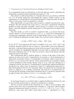
The MAE for the pure collaborative filtering method is 0.7597 and the coverage
98.34%. The MAE value for collaborative filtering method (without the neighborhood size restriction) is 0.7654 and the respective coverage 99.2%. The p-value
of the Wilcoxon test (p D 0:0002) indicates a statistically significant difference
suggesting that the restriction to produce prediction for a movie only if the neighbourhood consists of at least 5 neighbours lead to more accurate predictions, but
scarifies a portion of coverage.


22
Table 1 Number of features
and prediction accuracy

G. Lekakos et al.

Case
1
2
3
4
5

Threshold
(movies)
2
3

5
10
15

MAE
0.9253
0.9253
0.9275
0.9555
0.9780

Number
of features
10626
10620
7865
5430
3514

The pure content-based predictor presents MAE value 0.9253, which is significantly different (p D 0:000) than collaborative filtering. The coverage is 100%,
since content-based predictions ensures that prediction can always be produced for
every movie (provided that the target user has rated at least one movie). In the above
experiment we used a word as a feature if it appeared in the description of at least
two movies. We calculated the accuracy of the predictions when this threshold value
is increased to three, five, ten and fifteen movies, as shown in Table 1.
Comparing cases 1 and 2 above we notice no significant differences, while the
difference between 2 and 3, 4, 5 (p D 0:0000 for all cases) cases are statistically
significant.
Thus, we may conclude that the number of features that are used to represent the
movies is an important factor of the accuracy of the recommendations and, more

specifically, the more features are used, the more accurate the recommendations
are. Note that Naăve Bayes algorithm performed poorly in terms of accuracy with
ı
MAE D 1:2434. We improved its performance when considered ratings above 3 as
positive ratings and below 3 as negative (MAE D 1:118). However, this error is still
significantly higher than the previous implementation and therefore we exclude it
from the development of the hybrid approaches.
Substitute hybrid recommendation method was designed to achieve 100% coverage. The MAE of the method was calculated to be 0.7501, which is a statistically important improvement of the accuracy of pure collaborative filtering (p < 0:00001).
The coverage of the switching hybrid recommendation method is 98.8%, while
the MAE is 0.7702, which is a statistically different in relevance to substitute hybrid and pure collaborative filtering methods (p D 0:000). This method produces
recommendations of less accuracy than both pure collaborative filtering and substitute hybrid, has greater coverage than the first and lower that the latter method,
but it produces recommendations in reduced time than both methods above. Even
though recommendation methods are usually evaluated in terms of accuracy and
coverage, the reduction of execution time might be considered more important for
a recommender system designer, in particular in a system with a large number of
users and/or items.
Table 2 depicts the MAE values, coverage and time required for real-time prediction (on a Pentium machine running at 3.2 GHz with 1 GB RAM) for all four
recommendation methods.
Note that the most demanding algorithm in terms of resources for real-time prediction is collaborative filtering. If similarities are computed between the target and


1 Personalized Movie Recommendation
Table 2 MAE, coverage,
and prediction time for the
recommendation methods

Pure Collaborative
Filtering
Pure Content-based
Recommendations

Substitute hybrid
recommendation
method
Switching hybrid
recommendation
method

23

MAE
0.7597

Coverage
98.34%

run time
prediction
14 sec

0.9253

100%

3 sec

0.7501

100%

16 sec

0.7702

98.8%

10 sec

the remaining users at prediction time then its complexity is O .nm/ for n users
and m items. This may be reduced at O .m/ if similarities for all pairs or users are
pre-computed with an off-line cost O n2 m . However, such a pre-computation step
affects one of the most important characteristics of collaborative filtering, which is
its ability to incorporate the most up-to-date ratings in the prediction process. In
domains where rapid changes in user interests are not likely to occur the off-line
computation step may be a worthwhile alternative.

Conclusions and Future Research
The above empirical results provide useful insights concerning collaborative and
content-based filtering as well as their combination under the substitute and switching hybridization mechanisms.
Collaborative filtering remains one of the most accurate recommendation methods but for very large datasets the scalability problem may be considerable and a
similarities pre-computation phase may reduce the run-time prediction cost. The
size of target user’s neighbourhood does affect the accuracy of recommendations.
Setting the minimum number of neighbors to 5 improves prediction accuracy but at
a small cost in coverage.
Content-based recommendations are significantly less accurate than collaborative filtering, but are produced much faster. In the movie recommendation domain,
the accuracy depends on the number of features that are used to describe the movies.
The more features there are, the more accurate the recommendations.
Substitute hybrid recommendation method improves the performance of collaborative filtering in both terms of accuracy and coverage. Although the difference
in coverage with collaborative filtering on the specific dataset and with specific
conditions (user rated at least 20 movies, zero weight threshold value) is rather insignificant, it has been reported that this is not always the case, in particular when
increasing the weight threshold value [32]. On the other hand, the switching hybrid

24

G. Lekakos et al.

recommendation method fails to improve the accuracy of collaborative filtering, but
significantly reduces execution time.
The MoRe system is specifically designed for movie recommendations but its
collaborative filtering engine may be used for any type of content. The evaluation
of the algorithms implemented in the MoRe system was based on a specific dataset
which limits the above conclusions in the movie domain. It would be very interesting
to evaluate the system on alternative datasets in other domains as well in order to
examine the generalization ability of our conclusions.
As future research it would also be particularly valuable to perform an experimental evaluation of the system, as well as the proposed recommendations methods,
by human users. This would allow for checking whether the small but statistically
significant differences on recommendation accuracy are detectable by the users.
Moreover, it would be useful to know which performance factor (accuracy, coverage or execution time) is considered to be the most important by the users, since
that kind of knowledge could set the priorities of our future research.
Another issue that could be subject for future research is the way of the recommendations presented to the users, the layout of the graphical user interface and
how this influences the user ratings. Although there exist some studies on these issues (e.g. [34]), it is a fact that the focus in recommender system research is on the
algorithms that are used in the recommendation techniques.

References
1. D. Goldberg, D. Nichols, B.M. Oki, and D. Terry, “Using Collaborative Filtering to Weave an
Information Tapestry,” Communications of the ACM Vol. 35, No. 12, December, 1992, p.p.
61-70.
2. U. Shardanand, and P. Maes, “Social Information Filtering: Algorithms for Automating “Word
of Mouth”,” Proceedings of the ACM CH’95 Conference on Human Factors in Computing
Systems, Denver, Colorado, 1995, p.p. 210-217.

3. B. N. Miller, I. Albert, S. K. Lam, J. Konstan, and J. Riedl, “MovieLens Unplugged:
Experiences with an Occasionally Connected Recommender System,” Proceedings of the International Conference on Intelligent User Interfaces, 2003.
4. W. Hill, L. Stead, M. Rosenstein, and G. Furnas, “Recommending and Evaluating Choices
in a Virtual Community of Use,” Proceedings of the ACM Conference on Human Factors in
Computing Systems, 1995, p.p. 174-201.
5. Z. Yu, and X. Zhou, “TV3P: An Adaptive Assistant for Personalized TV,” IEEE Transactions
on Consumer Electronics, Vol. 50, No. 1, 2004, p.p. 393-399.
6. D. O’Sullivan, B. Smyth, D. C. Wilson, K. McDonald, and A. Smeaton, “Improving the
Quality of the Personalized Electronic Program Guide,” User Modeling and User Adapted
Interaction;Vol. 14, No. 1, 2004, p.p. 5-36.
7. S. Gutta, K. Kuparati, K. Lee, J. Martino, D. Schaffer, and J. Zimmerman, “TV Content
Recommender System,” Proceedings of the Seventeenth National Conference on Artificial
Intelligence, Austin, Texas, 2000, p.p. 1121-1122.
8. P. Resnick, N. Iacovou, M. Suchak, P. Bergstrom, and J. Riedl, “GroupLens: An Open Architecture for Collaborative Filtering of NetNews,” Proceedings of the ACM Conference on
Computer Supported Cooperative Work, 1994, p.p. 175-186.


1 Personalized Movie Recommendation

25

9. J. Konstan, B. Miller, D. Maltz, J. Herlocker, L. Gordon, and J. Riedl, “GroupLens: Applying
Collaborative Filtering to Usenet News,” Communications of the ACM, Vol. 40, No. 3, 1997,
p.p. 77-87.
10. G. Linden, B. Smith, and J. York, “Amazon.com Recommendations: Item-to-Item Collaborative Filtering,” IEEE Internet Computing, Vol. 7, No. 1, January-February, 2003, p.p. 76-80.
11. G. Lekakos, and G. M. Giaglis, “A Lifestyle-based Approach for Delivering Personalized
Advertisements in Digital Interactive Television,” Journal Of Computer Mediated Communication, Vol. 9, No. 2, 2004.
12. B. Smyth, and P. Cotter, “A Personalized Television Listings Service,” Communications of the
ACM;Vol.43, No. 8, 2000, p.p. 107-111.
13. G. Lekakos, and G. Giaglis, “Improving the Prediction Accuracy of Recommendation

Algorithms: Approaches Anchored on Human Factors,” Interacting with Computers, Vol. 18,
No. 3, May, 2006, p.p. 410-431.
14. J. Schafer, D. Frankowski, J. Herlocker, and S. Shilad, “Collaborative Filtering Recommender
Systems,” The Adaptive Web, 2007, p.p. 291-324.
15. J. S. Breese, D. Heckerman, and D. Kadie, “Empirical Analysis of Predictive Algorithms for
Collaborative Filtering,” Proceedings of the Fourteenth Annual Conference on Uncertainty in
Artificial Intelligence, July, 1998, p.p. 43-52.
16. J. Herlocker, J. Konstan, and J. Riedl, “An Empirical Analysis of Design Choices in
Neighborhood-Base Collaborative Filtering Algorithms,” Information Retrieval, Vol. 5, No.
4, 2002, p.p. 287-310.
17. K. Goldberg, T. Roeder, D. Guptra, and C. Perkins, “Eigentaste: A Constant-Time Collaborative Filtering Algorithm,” Information Retrieval, Vol. 4, No. 2, 2001, p.p. 133-151.
18. R. J. Mooney, and L. Roy, “Content-based Book Recommending Using Learning for Text
Categorization,” Proceedings of the Fifth ACM Conference in Digital Libraries, San Antonio,
Texas, 2000, p.p. 195-204.
19. M. Balabanovic, and Y. Shoham, “Fab: Content-based Collaborative Recommendation,” Communications of the ACM, Vol. 40, No. 3, 1997, p.p. 66-72.
20. M. Pazzani, and D. Billsus, “Learning and Revising User Profiles: The identification of interesting Web sites,” Machine Learning, Vol. 27, No. 3, 1997, p.p. 313-331.
21. M. Balabanovic, “An Adaptive Web Page Recommendation Service,” Proceedings of the ACM
First International Conference on Autonomous Agents, Marina del Ray, California, 1997, p.p.
378-385.
22. M. Pazzani, and D. Billsus, “Content-based Recommendation Systems,” The Adaptive Web,
2007, p.p. 325-341.
23. B. Sarwar, G. Karypis, J. Konstan, and J. Riedl, “Analysis of Recommendation Algorithms for
E-Commerce,” Proceedings of ACM E-Commerce, 2000, p.p. 158-167.
24. R. Burke, “Hybrid Recommender Systems: Survey and Experiments,” User Modeling and
User Adapted Interaction, Vol. 12, No. 4, November, 2002, p.p. 331-370.
25. M. Claypool, A. Gokhale, T. Miranda, P. Murnikov, D. Netes, and M. Sartin,
“Combining Content-Based and Collaborative Filters in an Online Newspaper,” Proceedings of the ACM SIGIR Workshop on Recommender Systems, Berkeley, CA, 1999,
ian/sigir99-rec/.
26. I. Schwab, W. Pohl, and I. Koychev, “Learning to Recommend from Positive Evidence,” Proceedings of the Intelligent User Interfaces, New Orleans, LA, 2000, p.p. 241-247.
27. M. Pazzani, “A Framework for Collaborative, Content-Based and Demographic Filtering,”

Artificial Intelligence Review, Vol. 13, No. 5-6, December, 1999, p.p. 393-408.
28. R. Burke, “Hybrid Web Recommender Systems,” The Adaptive Web, 2007, p.p. 377-408.
29. C. Basu, H. Hirsh, and W. Cohen, “Recommendation as Classification: Using Social and
Content-based Information in Recommendation,” Proceedings of the Fifteenth National Conference on Artificial Intelligence, Madison, WI, 1998, p.p. 714-720.
30. J. Alspector, A. Koicz, and N. Karunanithi, “Feature-based and Clique-based User Models for
Movie Selection: A Comparative study,” User Modeling and User Adapted Interaction, Vol. 7,
no. 4, September, 1997, p.p. 297-304.


26

G. Lekakos et al.

31. A. Rashid, I. Albert, D. Cosley, S. Lam, McNee S., J. Konstan, and J. Riedl, “Getting to Know
You: Learning New User Preferences in Recommender Systems,” Proceedings of International
Conference on Intelligent User Interfaces, 2002.
32. J. Herlocker, J. Konstan, A. Borchers, and J. Riedl, “An Algorithmic Framework for Performing Collaborative Filtering,” Proceedings of the Twenty-second International Conference
on Research and Development in Information Retrieval (SIGIR ’99), New York, 1999, p.p.
230-237.
33. G. Karypis, “Evaluation of Item-Based Top-N Recommendation Algorithms,” Proceedings
the Tenth International Conference on Information and Knowledge Management, 2001, p.p.
247-254.
34. D. Cosle, S. Lam, I. K. Albert, J., and J. Riedl, “Is Seeing Believing? How Recommender Systems Influence Users’ Opinions,” Proceedings of the SIGCHI Conference on Human Factors
in Computing Systems, Fort Lauderdale, FL, 2003, p.p. 585-592.


Chapter 2

Cross-category Recommendation
for Multimedia Content

Naoki Kamimaeda, Tomohiro Tsunoda, and Masaaki Hoshino

Introduction
Nowadays, Internet content has increased manifold not only in terms of Web site
categories but also other categories such as TV programs and music content. As of
2008, the total number of Web sites in the world exceeded 180 million [1]. Including
satellite broadcasting programs, there are thousands of channels in the TV program category. Consequently, in several categories, information overload and the
size of database storage are often acknowledged as problems. From the viewpoint
of such problems, there is a need for personalization technologies. By using such
technologies, we can easily find favorite content and avoid storing unnecessary content, because these technologies can select content that interests the user among a
large variety of content.
Recommendation services are one of the most popular applications that are
based on personalization technologies. Most of these services provide recommendations for individual categories. By applying recommendation technologies to several
different categories, user experience can be improved. By using user preferences involving several categories, the system can figure out more profound nature of user’s
taste and user’s view point to select content. Moreover, it becomes easier to find
similar content from other categories. In this article, this kind of recommendation is
referred to as “cross-category recommendation.”
The purpose of this article is to introduce cross-category recommendation technologies for multimedia content. First, in order to understand how to realize the
recommendation function, multimedia content recommendation technologies and
cross-category recommendation technologies are outlined. Second, practical applications and services using these technologies are described. Finally, difficulties involving cross-category recommendation for multimedia content and future
prospects are mentioned as the conclusion.
N. Kamimaeda ( ), T. Tsunoda, and M. Hoshino
Sec. 5, Intelligence Application Development Dept., Common Technology Division, Technology
Development Group, Corporate R&D, Sony Corporation, Tokyo, Japan
e-mail: ; ;
B. Furht (ed.), Handbook of Multimedia for Digital Entertainment and Arts,
DOI 10.1007/978-0-387-89024-1 2, c Springer Science+Business Media, LLC 2009

27

28

N. Kamimaeda et al.

Technological Overview
Overview
The technological overview is described in two parts: multimedia content recommendation technologies and cross-category recommendation technologies. The
relationship between these technologies is shown in Figure 1.
Multimedia recommendation technologies involve basic technologies that can be
used to realize recommendation functions for each category. Cross-category recommendation technologies involve technologies to realize cross-recommendation
among categories based on multimedia recommendation technologies. These two
technologies have been explained in the following sections.

Multimedia Content Recommendation
In this section, an overview of recommendation technologies for multimedia content is described. There are two types of such technologies: collaborative filtering
(CF) and content-based filtering (CBF). First, basic technologies about CF are described. Second, we explain CBF technologies in detail, because in this article, we
mainly explain cross-category recommendation technologies using CBF technologies. After that, typical cases of multimedia content recommendation systems are
mentioned. Finally, how to realize cross-category recommendation based on CBF
technologies is described.

Fig. 1 Two types of recommendation technologies


2 Cross-category Recommendation for Multimedia Content

29

Basic Technologies Involving CF
Collaborative filtering methods can be categorized into the following two types.

One type of CF starts by finding a set of customers whose purchases and rated items
overlap the user’s purchases and rated items [2]. The algorithm aggregates items
from such similar customers, eliminates items the user has already purchased or
rated, and recommends the remaining items to the user. This is called user-based
CF. Cluster models are also a type of user-based approach.
The other type of CF focuses on finding similar items, and not similar customers.
For each of the user’s purchased and rated items, the algorithm attempts to find similar items. It then aggregates the similar items and recommends them. This is called
item-based CF. Two popular versions of this algorithm are search-based methods
and item-to-item collaborative filtering [3].
Both CF methods cannot often work well with completely new items, items with
less reusability such as TV programs, high merchandise turnover rate items, and so
on. As a simple example of conventional CF, a problem in TV program recommendation can be encountered as follows.
1. Tom watched TV programs named X, Y, and Z.
2. Mike watched TV programs named X and Y but did not watch Z.
3. The system recommends program Z to Mike since Tom and Mike have watched
the same programs X and Y, but Mike has never watched program Z before.
4. However, program Z has already been broadcast and Mike cannot watch program
Z now.
Although CF methods have this type of problem, CF can be easily applied to
cross-category recommendation, because CF is independent of the type of item,
but it depends on which items are purchased or rated together. Moreover, technologies using community trends like CF are very important for cross-category
recommendation.
Lately, several community-based recommendation services have emerged.
Last.fm [4], MusicStrands (Mystrands) [5], and Soundflavor [6] are examples
of community-based music recommendation services. These sites obtain the listening logs or playlist data of community members; these song playlists are shared
with other community members and are also used to recommend music.

Basic Technologies Involving CBF
Key Elements of a Content Recommendation System Using CBF
A content recommendation system using CBF technologies has four key elements,

as shown in Figure 2: content profiling, context learning, user preference learning,
and matching.
In content profiling, the machine should understand what the content is in order
to recommend it. For example, jazz music has acoustic instrumentation and makes
for very relaxed listening. Understanding the content seems like an oversimplifica-


30

N. Kamimaeda et al.

Fig. 2 Four key elements of a CBF-based content recommendation system

tion, but a machine should manage all the necessary information that represents the
content. The next element is context learning. Understanding the user’s context is
also important for recommending content. The user’s interest is influenced by where
she/he is, the time of the day, what type of situation she/he is in, or how she/he is
feeling. For example, if the user is sitting in a caf´ near a tropical seashore, she/he
e
may prefer to listen to Latin music with a tropical cocktail in his/her hand. Alternatively, the user may prefer to listen to a wide range of music—classic to punk
rock music—in the morning. The third element is learning the users’ preferences.
Learning and understanding the user’s taste or preference is important to provide excellent recommendation in order to achieve better user satisfaction. If a user always
listens to songs sung by female vocalists, she/he may prefer vocal to instrumental
music. The last element is matching. Matching methods are used for recommending or searching relevant content. This key element measures the relevancy between
the three abovementioned entities, such as that between user preference and content
profile and the similarity between content.
In this chapter, these four key elements are discussed in detail; however, let us
briefly introduce other factors such as association discovery, trend discovery (TD),
and community-based recommendation. TD is useful from the viewpoint of providing recommendations because users often may wish to check the latest popular
trends. For example, the TD system extracts trends from the World Wide Web

(WWW) by employing a text mining technique comprising the following steps: (1)
identifying frequent phrases, (2) generating histories or phrases, and (3) seeking
temporal patterns that match a specific trend [7]. One research group has focused on
detecting the sentimental information associated with retail products by employing
natural language processing [8].


2 Cross-category Recommendation for Multimedia Content

31

Content Profiling
Content profiling can be considered as the addition of metadata that represents the
content or indexing it for retrieval purposes. It is often referred to as tagging, labeling, or annotation. Essentially, there are two types of tagging methods—manual
tagging and automatic tagging. In manual tagging, the metadata is manually fed as
the input by professionals or voluntary users. In automatic tagging, the metadata is
generated and added automatically by the computer. In the case of textual content,
keywords are automatically extracted from the content data by using a text mining
approach. In the case of audiovisual (AV) content, various features are extracted
from the content itself by employing digital signal processing technologies. However, even in the case of AV content, text mining is often used to assign keywords
from the editorial text or a Web site. In both manual and automatic approaches, it
is important for the recommendation system to add effective metadata that can help
classify the user’s taste or perception. For example, with respect to musical content,
the song length may not be important metadata to represent the user’s taste.

Manual Tagging
Until now, musical content metadata (Figure 3) have been generated by manual
tagging. All Media Guide (AMG) [9] offers a musical content metadata by professional music critics. They have over 200 mood keywords for music tracks. They
classify each music genre into hundreds of subgenres. For example, rock music has
over 180 subgenres. AMG also stores some emotional metadata, which is useful

to analyze artist relationships, search similar music, and classify the user’s taste in
detail. However, the problem with manual tagging is the time and cost involved.
Pandora [10] is well known for its personalized radio channel service. This service
is based on manually labeled songs from the Music Genome Project; according to
their Web site, it took them 6 years to label songs from 10,000 artists, and these
songs were listened to and classified by musicians. According to the AMG home
page, they have a worldwide network of more than 900 staff and freelance writers
specializing in music, movies, and games.
Similarly, Gracenote [11] has also achieved huge commercial success as a music
metadata provider. The approach involves the use of voluntary user input and the
service—compact disc database (CDDB)—is a de facto standard in the music metadata industry for PCs and mobile music players. According to Gracenote’s Web site,
the CDDB already contains the metadata for 55 million tracks and 4 million CDs
spanning more than 200 countries and territories and 80 languages; interestingly,
Gracenote employs less than 200 employees. This type of approach is often referred
to as user-generated content tagging.


32

N. Kamimaeda et al.

Fig. 3 Example of a song’s
metadata

Automatic Tagging
1) Automatic Tagging from Textual Information
In textual-content-based tagging, key terms are extracted automatically from the
textual content. This technique is used for extracting keywords not only from the
textual content but also from the editorial text; this explains its usability with respect
to tagging the AV content. “TV Kingdom” [12] is a TV content recommendation

service in Japan; it extracts specific keywords from the description text provided in
the electronic program guide (EPG) data and uses it as additional metadata. This is
because the EPG data provided by the supplier are not as effectively structured as
metadata and are therefore insufficient for recommendation purposes [13]. TV Kingdom employs the term frequency/inverse document frequency (TF/IDF) method to
extract keywords from the EPG. TF/IDF is a text mining technique that identifies
individual terms in a collection of documents and uses them as specific keywords.
The TF/IDF procedure can be described as follows:
Step 1: Calculate the term frequency (tf ) of a term in a document.
freq.i; j / D frequency of occurenceof term ti indocument Dj
The following formula is practically used to reduce the impact of highfrequency terms.
tfji D log.1 C freq.i; j //
Step 2: Calculate the inverse document frequency (idf ): idf i reflects the presumed
importance of term ti for the content representation in document Dj .
N
idf i D ni


2 Cross-category Recommendation for Multimedia Content

33

where
ni D number of documents in the collection to which term tj is assigned.
N D collection size:
The following formula is practically used to reduce the impact of large
values.
Á
N
idf i D log n
i

Step 3: The product of each factor is applied as the weight of the term in this document.
wj D tfij idf i
i
Google [14] is the most popular example of automatic tagging based on textual
information. Google’s Web robots are software modules that crawl through the Web
sites on the Internet, extract keywords from the Web documents, and index them
automatically by employing text mining technology. These robots also label the
degree of importance of each Web page by employing a link structure analysis; this
is referred to as Page Rank [15].
2) Automatic Tagging from Visual Information
Research on content-based visual information retrieval systems has been undertaken
since the early 1990s. These systems extract content features from an image or
video signal and index them. Two types of visual information retrieval systems exist.
One is “query by features”; here, sample images or sketches are used for retrieval
purposes. The other is “query by semantics”; here, the user can retrieve visual information by submitting queries like “a red car is running on the road.”
Adding tags to image or video content is more complex than adding tags to textual content. Certain researches have suggested that video content is more complex
than a text document with respect to six criteria: resolution, production process,
ambiguity in interpretation, interpretation effort, data volume, and similarity [16].
For example, the textual description of an image only provides very abstract details. It is well known that a picture is worth a thousand words. Furthermore, video
content—a temporal sequence of many images—provides higher-level details that a
text document cannot yield. Therefore, query by semantics, which is a content-based
semantic-level tagging technique, is still a complex and challenging topic. Nevertheless, query-by-feature approaches such as QBIC and VisualSEEK achieve a certain
level of performance with regard to visual content retrieval [17], [18]. This approach
extracts various visual features including color distribution, texture, shape, and spatial information, and provides similarity-based image retrieval; this is referred to as
“query by example.”
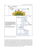
In order to search for a similar image, the distance measure between images
should be defined in the feature space, and this is also a complex task. A simple
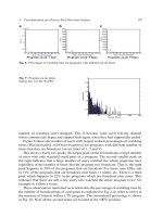
example of distance measure using color histograms is shown in Figure 4 in order
to provide an understanding of the complexity involved in determining the similarity between images. This figure shows three grayscale images and their color
histograms in Panel a, Panel b, and Panel c. It may appear that Image (b) is similar

34

N. Kamimaeda et al.

Fig. 4 Typical grayscale image sample

Fig. 5 Minkowski distance measure

to Image (a) rather than Image (c). However, simple Minkowski distance reveals that
Image (b) has greater similarity to Image (c) than Image (a), as shown in Figure 5.
There exists a semantic gap between this distance measure and human perception.
In order to overcome this type of problem, various distance measures have been
proposed, such as earth mover’s distance (EMD) [19]. JSEG outlines a technique
for spatial analysis using the image segmentation method to determine the typical
color distributions of image segments. [20].
In addition to the global-color-based features mentioned above, image recognition technology is also useful for image tagging. A robust recognition algorithm of object recognition from multiple viewpoints has also been proposed [21].
The detection and indexing of objects contained in images enable the query-byexample service with a network-connected camera such as one on a mobile phone.
Face recognition and detection technologies also have potential for image tagging.
Sony’s “Picture Motion Browser” [22] employs various video feature extraction


2 Cross-category Recommendation for Multimedia Content

35

technologies including face-recognition to provide smart video browsing features
such as personal highlight search and video summarization. A hybrid method merging both local features from image recognition technology and global-color-based
feature will enhance the accuracy of image retrieval.

Many researches pursue the goal of sports video summarization because sports
video has a typical and predictable temporal structure and recurring events of similar
types such as corner kicks and shots at goal in soccer games. Furthermore, consistent
features and fixed number of views allow us to employ less complex content model
than those necessary for ordinary movie or TV drama content. Most of the solutions
involve the combination of the specific local features such as line mark, global visual
features and also employ audio features such as high-energy audio segment.
3) Automatic Tagging from Audio Information
In addition to images, there are various approaches for achieving audio feature
extraction by employing digital signal processing. In the MPEG-7 standard, audio
features are split into two levels—“low-level descriptor” and “high-level descriptor.”
However, a “mid-level descriptor” is also required to understand automatic tagging
technologies for audio information. Low-level features are signal-parameter-level
features such as basic spectral features. Mid-level features are musical-theory-level
features, for example, tempo, key, and chord progression, and other features such as
musical structure (chorus part, etc.), vocal presence, and musical instrument timbre.
High-level features such as mood, genre, and activity are more generic.
The EDS system extracts mid- and high-level features from an audio signal [23].
It involves the generation of high-level features by combining low-level features.
The system automatically discovers an optimal feature extractor for the targeted
high-level features, such as the musical genre, by employing a machine learning
technology. The twelve-tone analysis is an alternative approach for audio feature
extraction; it analyzes the audio signal based on the principles of musical theory.
The baseband audio signal is transformed into the time–frequency domain and split
into 1/12 octave signals. The system can extract mid- and high-level features by
analyzing the progression of the twelve-tone signal patterns. Sony’s hard-disk-based
audio system “Giga Juke” [24] provides smart music browsing capabilities based on
features such as mood channel and similar song search by the twelve-tone analysis.
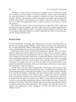
Musical fingerprinting (FP) also extracts audio features, but it is used for accurate music identification rather than for retrieving similar music. Figure 6 shows the
framework of the FP process [25]. Similar to the abovementioned feature extraction

procedures, FP extracts audio features by digital signal processing, but it generates
a more compact signature that summarizes an audio recording. FP is therefore capable of satisfying the requirements of both fast retrieval performance and compact
footprint to reduce memory space overhead. Gracenote and Shazam [26] are two
well-known FP technologies and music identification service providers.


36

N. Kamimaeda et al.

Fig. 6 FP framework

Context Learning
A mobile terminal is a suitable device for detecting the user’s context because it is
always carried by the user. In the future, user contexts such as time, location, surrounding circumstances, personal mood, and activity can be or will be determined
by mobile terminals. Therefore, if the user context can be identified, relevant information or context-suitable content can be provided to the user.
The user’s location (physical position) can be easily detected by employing a
GPS-based method or cell-network-based positioning technology. The latter encompasses several solutions such as timing advance (CGICTA), enhanced CGI (E-CGI),
cell ID for WCDMA, uplink time difference of arrival (U-TDOA), and any time
interrogation (ATI) [27]. The detection of the surrounding circumstances is a challenging issue. One of the approaches has proposed the detection of the surrounding
circumstances by using ambient audio and video signals [28]. A 180ı wide-angle
lens is used for visual pattern learning for different circumstances or events such
as walking into a building or walking down a busy street. Personal mood detection
is also an interesting and challenging topic. Nowadays, gyrosensor (G-sensor) devices are used in commercial computer gaming systems, wherein user movement
can be detected; G-sensors can therefore detect user activity such as whether she/he
is running, walking, sitting, or dancing.
User Preference Learning
User preferences can be understood by studying the user’s response to the content.
A computer system cannot understand user tastes without accessing user listening
and watching logs or acquiring certain feedback. For example, people who always

listen to classical and ethnic music may prefer such genres and might seem to prefer
acoustic music over electronic music. People who read the book “The Fundamentals
of Financing” might be interested in career development or might attempt to invest
in some venture capitals to avail of a high return for their investments.


2 Cross-category Recommendation for Multimedia Content

37

To realize this type of user preference learning, the system must judge whether
the user’s feedback regarding the content is positive or negative. After judging
whether the feedback provided is positive or negative, the system can learn the
user’s preferences based on the content’s metadata. There are two types of user
feedback—explicit and implicit. “Initial voluntary input of a user’s preference regarding the registration process” or “clicking the like/dislike button” are examples
of explicit feedback. “Viewing detailed information on the content,” “purchasing
logs of an e-commerce site,” and “operation logs such as play or skip buttons for AV
content” are examples of implicit feedback. Generally, the recommendation systems
emphasize upon explicit rather than implicit feedback.
After the “like” or “dislike” rating is determined, the system adds or subtracts certain points to or from each attribute, respectively. In a “vector space model” (VSM)
(introduced later), the user preference is expressed as an n-dimensional attribute
vector based on this process. In the probabilistic algorithm (also introduced in the
subsequent section), user preference is expressed in terms of probabilistic parameters in addition to the attribute value. For example, if a user is satisfied with 60
jazz songs per 100 recommended songs, the probabilistic parameter is expressed as
P(likejgenre D jazz/ D 60=100 D 0:6.
Matching
There are two types of matching approaches—exact matching and similarity matching. The former seeks contents with the same metadata as that of the search query,
such as keywords or tags. The latter seeks contents with metadata similar to that of
the search query. In this section, two types of similarity calculation methodsVSM
and naăve Bayesian classier (NB)are introduced; however, there are several

other exact matching and similarity matching methods.

1) VSM
One of the simplest approaches for similarity calculation is using the VSM. This
model measures the distance between vectors. The most practical distance measure
is the cosine distance, as shown in Figure 7. For example, user preference (UP) and

Fig. 7 Example of Similarity
in VSM


38

N. Kamimaeda et al.

content profile (CP) are expressed as an n-dimensional feature vector in the VSM.
The similarity between UP and CP is usually defined as follows:
Á
E E
U C
E E
si m U ; C D cos  D
E E
jU jjC j
where
E
U D .u1 ; u2 ; ; ; un / user preference vector
E
C D .c1 ; c2 ; ; ; cn / contents profile vector

2) NB Classifier
NB is a probabilistic approach to classify data or infer a hypothesis. It is also
practically used in recommendation systems [29]. Let us apply NB to measure the
similarity between user preference and content profile. In NB, the initial probabilities of the user’s tastes are determined from the training data. For example, if a
user is satisfied with 60 jazz songs per 100 recommended songs, the conditional
probability P(likejgenre D jazz) D 0.6. If she/he is satisfied with 80 acoustic songs
per 100 recommended songs, P(like j timbre D acoustic) D 0.8. Therefore, we can
hypothesize that the user likes acoustic jazz music. After the learning phase, NB
can classify the new songs based on the user’s tastes, i.e., whether she/he likes these
songs or not. For this, NB calculates which class maximizes P .cjs/, as shown in
(1); here, s is the content vector expressed in terms of the attribute values (a1, a2,
a3,. . . , an).
c D arg max P .cjE/ D arg max
O
s
c

c

P .Ejc/P .c/
s
D arg max P .c/P .Ejc/
s
P .E/
s

(1)

where

c D estimated class (like or dislike)
O
c D class (like or dislike)
s D .a1 ; a2 ; ; ; ; an / content (song) vector expressed by its attribute vector.
E
Bayes theorem: The posterior probability p.hjD/ given D
P .hjD/ D

P .D= h/P .h/
P .D/

(2)

In (1), the probability P .c/ can be easily estimated by counting the frequency in the training phase. However, it is difficult to calculate P .sjc/ D
P .a1; a2; a3; : : :; anjc/. Since there are several possible combinations of attributes,
a large number of training sets is required. In order to resolve this problem, NB assumes a very simple rule: the values of the attributes are conditionally independent,
as shown in (2). Therefore, by substituting (3) in (1), NB can be simply expressed


2 Cross-category Recommendation for Multimedia Content

39

as (4). It is easy to determine P .c/ and P .ai jc/ as the user preference by using
explicit and implicit feedback provided by the user.
P .Ejc/ D P .a1 ; a2 ; ; ; an jc/ D
s

Y

P .ai jc/

(3)

i

c D arg max P .c/
O
c

Y

P .ai jc/

(4)

i

3) Other Approaches
The usage of VSM and NB both poses a problem referred to as “the curse of
dimension”: as the number of dimensions increases, the discrimination performance
deteriorates. Some of the approaches to avoid this problem are dimension reduction
(feature selection) and application of weight or bias to the attributes. Feature selection eliminates irrelevant or inappropriate attributes. Principal component analysis
(PCA) or probabiliistic latent semantic analysis (pLSA) can be used to this end.
The latter models a document as a combination of hidden variables which explain
its topics. In addition to dimension reduction, support vector machine (SVM) is
an effective and robust tool to classify data into two classes. The application of
weight or bias to the attributes based on individual user’s viewpoint has also been
proposed [30].
Typical Cases of Multimedia Content Recommendation System

There are several matching combinations for content recommendation systems, as
shown in Figure 8. Typically, four combinations are often used in recommendation

Fig. 8 Matching combinations for a content recommendation system


40

N. Kamimaeda et al.

systems. The first is “content-to-content matching,” referred to as “content-meta-based
search.” The second is “context-to-content matching,” also referred to as “contextaware search.” The third is “user-preference-to-content matching,” also referred to
as “user-preference-based search.” The last is “user-preference-to-user-preference
matching,” which is another case of “user-preference-based search.” This chapter
investigates three types of recommendation systems (shown in Figures 9, 10, and 11).

Fig. 9 Content-meta-based search

Fig. 10 Context-aware search

Fig. 11 User-preference-based search