Handbook of Multimedia for Digital Entertainment and Arts- P5 ppsx

4 Personalization on a Peer-to-Peer Television System

a

4

b

3.5 x 10

107

c

Count

Count

1.5

12000

5000

10000

4000

8000

3000

0.5

6000

2000

1

0
0

14000

6000

2

16000

7000
2.5

18000

8000

3

Count

9000

4000

1000
10 20 30 40 50 60 70 80 90 100
Wach Time (Percentage)

Programs on-air 1 time

0
0

2000
10 20 30 40 50 60 70 80 90 100
Wach Time (Percentage)

Programs on-air 5 times

0
0

10 20 30 40 50 60 70 80 90 100
Wach Time (Percentage)

Programs on-air 9 times

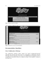
Fig. 8 Percentage of watching time for programs with different on-air times

Fig. 9 Program on-air times
during Jan.1 to Jan 30,2003

4
3.5

log(count)

3
2.5
2
1.5
1
0.5
0
0

50

100
150
On−air Times

200

250

number of watching users dropped. This is because some users left the channel
when commercials began and zapped back again when they had supposedly ended.
Figure 8 shows the number of users with respect to their percentages of watching

times (WatchLenght.k; m//OnAirlength(m)) for programs with different number of
times that they are broadcast (on-air times of 1, 5 and 9).
This shows clearly two peaks: the larger peak on the left indicates a large number
of users who only watched small parts of a program. The second smaller peak on
the right indicates that a large number of users watched the whole programs once
regardless of the number of times that the program was broadcast. That is, the right
peak happens in 20% of the programs that are broadcast five times (one fifth), and
in 11% of the programs that are broadcast nine times (1 ninth), etc. There is a third
peak which happens in 22% in the programs which are broadcast nine times. This
indicates that there are still a few users who watched the entire program twice, for
example to follow a series.
These observations motivated us to normalize the percentage of watching time by
the number of broadcastings of a program as explained in Eq. 2, in order to arrive at
the measure of interest within a TV program. This normalized percentage is shown
in Fig. 10. Now all the second peaks are located at the 100% position.


108

J. Wang et al.

Fig. 10 Normalized percentage of watching time

5.2
5

log(Count)

4.8
4.6

4.4
4.2
4
3.8
3.6
3.4
3.2

0

10 20 30 40 50 60 70 80 90 100
Watch %

Learning the User Interest Threshold
The threshold level, T , above which the normalized percentage of watching time is
considered to express interest in a TV program (Eq. (3)) is determined by evaluating
the performance of the recommendation for different setting of this threshold.
The recommendation performance is measured by using precision and recall of a
set of test users. Precision measures the proportion of recommended programs that
the user truly likes. Recall measures the proportion of the programs that a user truly
likes that are recommended. In case of making recommendations, precision seems
more important than recall. However, to analyze the behavior of our method, we
report both metrics on our experimental results.
Since we lack information on what the users liked, we considered programs that
a user watched more than once xk;m > 1 to be programs that the user likes and
all other programs as shows that the user does not like. Note that, in this way, only
a fraction of the programs that the user truly liked are caputered. Therefore, the
measured precision underestimates the true precision [Hull 1993].
For cross-validation, we randomly divided this data set into a training set (80%
of the users) and a test set (20% of the users). The training set was used to estimate

the model. The test set was used for evaluating the accuracy of the recommendations
on the new users, whose user profiles are not in the training set. Results are obtains
by averaging 5 different runs of such a random division.
We plotted the performance of recommendations (both precision and recall)
against the threshold on the percentage of watching time in Fig. 11. We also varied
the number of programs returned by the recommender (top-1, 10, 20, 40, 80 or 100
recommended TV programs). Figure 11(a) shows that in general, the threshold does
not affect the precision too much. For the large number of programs recommended,
the precision becomes slightly better when there is a larger threshold. For larger
number of recommended programs, the recall, however, drops for larger threshold
values (shown in Fig. 11(b)). Since the threshold does not affect the precision too
much, a higher threshold is chosen in order to reduce the length of the user interest profiles to be exchanged within the network. For that reason we have chosen a
threshold value of 0.8.


4 Personalization on a Peer-to-Peer Television System

b

a
Top−1 return
Top−10 return
Top−20 return
Top−40 return
Top−60 return
Top−80 return
Top−100 return

1

1
Top−1 return
Top−10 return
Top−20 return
Top−40 return
Top−60 return
Top−80 return
Top−100 return

0.9
0.8
Recommendation Recall

Recommendation Precision

1.2

109

0.8

0.6

0.4

0.7
0.6
0.5
0.4
0.3

0.2

0.2
0.1
0

0

0.1

0.2

0.3
0.4
0.5
0.6
0.7
Threshold (Percentage)

0.8

0.9

1

0

0

Precision of Recommendation

0.1

0.2

0.3 0.4
0.5 0.6
0.7
Threshold (Percentage)

0.8

0.9

1

Recall of Recommendation

Fig. 11 Recommendation performance v.s. threshold T

Convergence Behavior of BuddyCast
We have emulated our BuddyCast algorithm using a cluster of PCs (the DAS-24
system). The simulated network consisted of 480 users distributed uniformly over
32 nodes. We used the user profiles of 480 users. Each user maintained a list of
10 taste buddies .N D 10/ and the 10 last visited users .K D 10/. The system was
initialized by giving each user a random other user. The exploration-to- exploitation
ı was set to 1.
Figure 12 compares the convergence of BuddyCast to that of newscast (randomly
select connecting users, i.e., ı ! 1). After each update we compared the list of
top-N taste buddies with a pre-compiled list of top-N taste buddies generated using

all data (centralized approach). In Fig. 12, the percentage of overlap is shown as a
function of time (represented by the number of updates). The figure shows that the
convergence of Buddycast is much faster than that of the Newscast approach.

Recommendation Performance
We first studied the behavior of the linear interpolation smoothing for recommendation. For this, we plotted the average precision and recall rate for the different
values of the smoothing parameter i in the Audioscrobbler data set. This is shown
in Fig. 13.
Figure 13(a) and (b) show that both precision and recall drop when i reaches its
extreme values zero and one. The precision is sensitive to i , especially the early
precision (when only a small number of items are recommended). Recall is less
4

/>

110

J. Wang et al.

Fig. 12 Convergence of our buddycast algorithm

a

b
Top−1 return
Top−10 return
Top−20 return
Top−40 return

Top−1 return

Top−10 return
Top−20 return
Top−40 return

0.5

0.5

Recommendation Recall

Recommendation Precision

0.6

0.4

0.3

0.2

0.4

0.3

0.2

0.1

0.1
0

0.1

0.2

0.3

0.4

0.5
0.6
lambda

0.7

0.8

Precision of recommendation

0.9

1

0

0

0.1

0.2

0.3

0.4
0.5
lambda

0.6

0.7

0.8

0.9

1

Recall of recommendation

Fig. 13 Recommendation performance of the linear interpolation smoothing

sensitive to the actual value of this parameter, having its optimum at a wide range of
values. Effectiveness tends to be higher on both metrics when i is large; when i is
approximately 0.9, the precision seems optimal. An optimal range of i near one can
be explained by the sparsity of user profiles, causing the prior probability Pml .ib jr/
to be much smaller than the conditional probability Pml .ib jim ; r/. The background
model is therefore only emphasized for values of i closer to one. In combination
with the experimental results that we obtained, this suggests that smoothing the cooccurrence probabilities with the background model (prior probability Pml .ib jr/ /
improves recommendation performance.

4 Personalization on a Peer-to-Peer Television System
Table 1 Comparison of recommendation performance
Top-1 Item
Top-10 Item
(a) Precision
UIR-Item
0.62
0.52
Item-TFIDF
0.55
0.47
Item-CosSin
0.56
0.46
Item-CorSim
0.50
0.38
Item-CorSim
0.55
0.42
(b) Recall
UIR-Item
0.02
0.15
Item-TFIDF
0.02
0.15
Item-CosSin
0.02

0.13
Item-CorSim
0.01
0.11
Item-CorSim
0.02
0.15

111

Top-20 Item

Top-40 Item

0.44
0.40
0.38
0.33
0.34

0.35
0.31
0.31
0.27
0.27

0.25
0.26
0.22
0.19

0.25

0.40
0.41
0.35
0.31
0.39

Next, we compared our relevance model to other log-based collaborative filtering approaches. Our goal here is to see, using our user-item relevance model,
whether the smoothing and inverse item frequency should improve recommendation performance with respect to the other methods. For this, we focused on the
item-based generation (denoted as UIR-Item). We set i to the optimal value 0.9.
We compared our results to those obtained with the Top-N-suggest recommendation
engine, a well-known log-based collaborative filtering implementation5 [Deshpande
& Karypis 2004]. This engine implements a variety of log-based recommendation
algorithms. We compared our own results to both the item-based TF IDF-like
version (denoted as ITEM-TFIDF) as well the user-based cosine similarity method
(denoted as User-CosSim), setting the parameters to the optimal ones according to
the user manual. Additionally, for item-based approaches, we also used other similarity measures: the commonly used cosine similarity (denoted as Item-CosSim)
and Pearson correlation (denoted as Item-CorSim). Results are shown in Table 1.
For the precision, our user-item relevance model with the item-based generation
(UIR-Item) outperforms other log-based collaborative filtering approaches for all
four different number of returned items. Overall, TF IDF-like ranking ranks second. The obtained experimental results demonstrate that smoothing contributes to
a better recommendation precision in the two ways also found by [Zhai & Lafferty 2001]. On the one hand, smoothing compensates for missing data in the
user-item matrix, and on the other hand, it plays the role of inverse item frequency to
emphasize the weight of the items with the best discriminative power. With respect
to recall, all four algorithms perform almost identically. This is consistent to our first
experiment that recommendation precision is sensitive to the smoothing parameters
while the recommendation recall is not.

5

karypis/suggest/


112

J. Wang et al.

Conclusions
paper discussed personalization in a personalized peer-to-peer television system
called Tribler, i.e., 1) the exchange of user interest profiles between users by automatically creating social groups based on the interest of users, 2) learning these
user interest profiles from zapping behavior, 3) the relevance model to predict user
interest, and 4) a personalized user interface to browse the available content making
use of recommendation technology. Experiments on two real data sets show that
personalization can increase the effectiveness to exchange content and enables to
explore the wealth of available TV programs in a peer-to-peer environment.

References
Ali, K. & van Stam, W., (2004). TiVo: Making Show Recommendations Using a Distributed
Collaborative Filtering Architecture. International ACM SIGKDD Conference on Knowledge
Discovery and Data Mining.
Ardissono, L., Kobsa, A., & Maybury, M. (Ed). (2004). Personalized Digital Television. Targeting
programs to individual users. Kluwer Academic Publishers.
Breese, J. S., Heckerman, D., & Kadie, C., (1998). Empirical Analysis of Predictive Algorithms
for Collaborative Filtering. Conference on Uncertainty in Artificial Intelligence.
Claypool, M., Waseda, M., Le, P., & Brow, D. C., (2001). Implicit interest indicators. International
Conference on Intelligent User Interfaces.
Deshpande, M. & Karypis, G. (2004). Item-based top-n recommendation algorithms. ACM Transactions on Information Systems.
Eugster, P.T., Guerraoui, R., Kermarrec, A.M., & Massoulie, L. (2004), From epidemics to distributed computing, IEEE Computer. 21(3):341–374.
Eyheramendy, S., Lewis, D., & Madigan. D. (2003). On the naive bayes model for text categorization. In Proc. of Artificial Intelligence and Statistics.

Fokker, J.E. & De Ridder, H. (2005). Technical Report on the Human Side of Cooperating in Decentralized Networks. Internal report I-Share Deliverable 1.2, Delft University of Technology.
/>Hofmann, T. (2004). Latent Semantic Models for Collaborative Filtering. ACM Transactions on
Information Systems.
Herlocker, J.L., Konstan, J.A., Borchers, A., & Riedl J. (1999). An algorithmic framework for
performing collaborative filtering. International ACM SIGIR Conference on Research Development on Information Retrieval.
Hull. D. (1993). Using statistical testing in the evalution of retrieval experiments. International
ACM SIGIR Conference on Research Development on Information Retrieval.
Jelasity, M & van Steen, M. (2002). Large-Scale Newscast Computing on the Internet. Internal
report IR-503, Vrije Universiteit, Department of Computer Science.
Lafferty, J., & Zhai, C. (2003). Probabilistic relevance models based on document and query generation. In W. B. Croft and J. Lafferty, editors, Language Modeling and Information Retrieval.
Kluwer Academic Publishers.
Linden G., Smith, B., & York J. (2003). Amazon. com recommendations: item-to-item collaborative filtering. IEEE Internet Computing.
Linden G., Smith, B., & York J. (2003). Amazon. com recommendations: item-to-item collaborative filtering. IEEE Internet Computing.
Marlin B. (2004). Collaborative filtering: a machine learning perspective. Master’s thesis, Department of Computer Science, University of Toronto.


4 Personalization on a Peer-to-Peer Television System

113

Miller, B.M., Konstan, J.A., & Riedl, J. (2004) PocketLens: Toward a Personal Recommender
System. ACM Transactions on Information Systems.
Nichols, D. (1998). Implicit rating and filtering. In Proceedings of 5th DELOS Workshop on Filtering and Collaborative Filtering, pages 31-36, ERCIM.
Pouwelse, J. A., Garbacki, P., Wang, J., Bakker, A., Yang, J., Iosup, A., Epema, D.H.J, Reinders,
M.J.T van Steen, M., & Sips, H.J. (2005). Tribler: A social-based Peer-to-Peer system. International Workshop on Peer-to-Peer Systems (IPTPS’06).
Sarwar, B., Karypis, G., Konstan, J., & Riedl, J. (2001). Item-based collaborative filtering recommendation algorithms. International World Wide Web Conference.
Wang, J., de Vries, A.P., & Reinders, M.J.T, (2005a). A User-Item Relevance Model for Log-based
Collaborative Filtering. European Conference on Information Retrieval.
Wang, J., de Vries, A.P., & Reinders, M.J.T, (2006b). Unifying User-based and Item-based Collaborative Filtering by Similarity Fusion. International ACM SIGIR Conference on Research
Development on Information Retrieval.

Wang, J., Pouwelse, J., Lagendijk, R., & Reinders, M.J.T, (2006c). Distributed Collaborative Filtering for Peer-to-Peer File Sharing Systems, ACM Symposium on Applied Computing.
Xue, G, Lin, C., Yang, Q., Xi, W., Zeng, H., Yu, Y., & Chen. Z. (2005). Scalable Collaborative
Filtering Using Cluster-based Smoothing. International ACM SIGIR Conference on Research
Development on Information Retrieval.
Zhai. C., & Lafferty. J. (2001). A Study of Smoothing Methods for Language Models Applied to
Ad Hoc Information Retrieval. International ACM SIGIR Conference on Research Development on Information Retrieval.


Chapter 5

A Target Advertisement System Based on TV
Viewer’s Profile Reasoning
Jeongyeon Lim, Munjo Kim, Bumshik Lee, Munchurl Kim, Heekyung Lee,
and Han-kyu Lee

Introduction
With the rapidly growing Internet, the Internet broadcasting and web casting service have been one of the well-known services. Specially, it is expected that the
IPTV service will be one of the principal services in the broadband network [2].
However, the current broadcasting environment is served for the general public and
requires the passive attitude to consume the TV programs. For the advanced broadcasting environments, various research of the personalized broadcasting is needed.
For example, the current unidirectional advertisement provides to the TV viewers
the advertisement contents, depending on the popularity of TV programs, the viewing rates, the age groups of TV viewers, and the time bands of the TV programs
being broadcast. It is not an efficient way to provide the useful information to the
TV viewers from customization perspective. If a TV viewer does not need particular
advertisement contents, then information may be wasteful to the TV viewer. Therefore, it is expected that the target advertisement service will be one of the important
services in the personalized broadcasting environments. The current research in the
area of the target advertisement classifies the TV viewers into clustered groups who
have similar preference. The digital TV collaborative filtering estimates the user’s
favourite advertisement contents by using the usage history [1, 4, 5]. In these studies,
the TV viewers are required to provide their profile information such as the gender,

job, and ages to the service providers via a PC or Set-Top Box (STB) which is connected to digital TV. Based on explicit information, the advertisement contents are
provided to the TV viewers in a customized way with tailored advertisement contents. However, the TV viewers may dislike exposing to the service providers their
J. Lim ( ), M. Kim, B. Lee, and M. Kim
Information and Communications University,
119 Munji Street, Yuseong-gu,
Daejeon 305-732, Korea
e-mail: fjylim; kimmj; bslee;
H. Lee, and H.-K. Lee
Electronics and Telecommunications Research Institute, Daejeon, Korea
e-mail: flhk95;
B. Furht (ed.), Handbook of Multimedia for Digital Entertainment and Arts,
DOI 10.1007/978-0-387-89024-1 5, c Springer Science+Business Media, LLC 2009

115


116

J. Lim et al.

private information because of the misuse of it. In this case, it is difficult to provide
appropriate target advertisement service.
In this paper, we only utilize implicit information of TV usage history such as the
viewing date, viewing time, and genres for TV programs. We design a multi-stage
classifier as a profile reasoning algorithm for TV viewers. The proposed multi-stage
classifier is trained with real usage history data of 2,522 people for TV programs.
We also develop a target advertisement system based on the TV viewers’ profile
reasoning algorithm. The target advertisement system selects and provides relevant
commercials to the targeted groups. This paper is organized as follows: Section 5
presents the architecture of our target advertisement system with possible applications scenarios; Section 5 describes our proposed profile reasoning algorithm for

TV viewers, which classifies unknown TV viewers into an appropriate gender–age
group; Section 5 addresses a commercial selection method for target advertisement;
Plenty of experimental results are provided and analyzed for the profile reasoning
performance; and finally we conclude our work in concluding section.

Architecture of Proposed Target Advertisement System
In the proposed target advertisement service system, there are three major entities:
a content provider, advertisement companies, and TV viewers. The proposed target
advertisement system consists of the following necessary modules; a profile reasoning module to infer a TV viewer’s profile by analyzing their TV usage history,
a broadcasting transmission module to recommend services based on the inferred
result, and a user interface module to protect TV viewers’ profile. The terminals at
the TV viewers’ side send limited information with their TV usage history to the
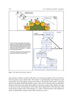
service provider (target advertisement system), and receives the selected commercials which are recommended by the target advertisement service system. Figure 1
shows the architecture of our proposed target advertisement system. The target advertisement system consists of three agents such as an inference agent of TV viewer
profiles which has the profile reasoning module for TV viewers, a content provision
agent which contains a selection module of appropriate TV commercials to the targeted TV viewers and a transmission module for TV program contents, and a user
interface agent which consists of an input interface module and a TV usage history
transmission module.
In Fig. 1, the profile inference agent of TV viewers receives the usage history
data of TV programs such as TV program titles, genres, channels, viewing times
band, and viewing days of the week from the user interface agent. By utilizing this
information, the profile inference agent infers the TV viewers’ profile in their preferred genres and time bands of TV viewing for the groups of different genders and
ages by the profile reasoning module, and the inference results are sent to the content provision agent. Based on the profile inference results, the content provision
agent selects appropriate commercial contents to unknown target TV viewers by the
advertisement content selection module. The selected commercial contents can be


5 A Target Advertisement System Based on TV Viewer’s Profile Reasoning

117

Broadcasting Station
Profile Inference Agent

Content Provider Agent

TV viewer Profile
Reasoning Module

Advertisement Contents
Selection Module

Reasoning Profile
* Gender
* Age

VOD
Work Place

Personalized contents
Ad content
DB

TV Usage
History DB

Advertisement
Content

TV Anytime

Metadata DB

* Preferred TV program
* Target Advertisement Contents

Advertisement
Company

Network
Set-Top Box
User Interface Agent
TV Usage History
TX Module

TV viewer Input
Interface Module

TV viewer
TV viewer’s input
* Start/Stop watching TV
* Select TV program/channel

TV Usage
History DB

Fig. 1 Target advertisement system architecture

distributed by the broadcasting station with TV program contents or VoD (Video
on Demand). The user interface agent provides a GUI which enables TV viewers
to consume contents or relative data at the TV terminal. The user interface agent

works on the STB (Set-Top Box) which enables the TV viewers to consume the recommended TV commercial contents with TV programs from the content provider
agent. While the TV viewers watch TV programs, the user interface agent stores the
usage data of the TV programs being watched into the TV usage history DB of STB
through the input interface module. By the level of information provision for the TV
program consumption, stored information is divided into TV usage information and
private information. Only a limited amount of information about TV program consumption is transmitted to the profile inference agent through the TV usage history
transmission module, which makes it possible to infer TV viewers’ profiles.

Proposed Profile Reasoning Algorithm
In this section, we describe a multi-stage classifier for the proposed profile reasoning
algorithm, and explain how to extract feature vectors in order to train the multi-stage
classifier.


118

J. Lim et al.

Analysis of Features Depending on User Profiles
The feature vector for profile reasoning algorithm can be obtained from the TV usage history. In this paper, we use usage history data of TV programs for male and
female TV viewers in different ages by AC Nielson Korea. The TV usage history
has various fields as shown in Table 1. The TV usage history was recorded by 2,522
people (Male: 1,243 and Female: 1,279) from Dec. 2002 to May, 2003. The TV programs are categorized into eight genres such as News, Information, Drama&Movie,
Entertainments, Sports, Education Child, and Miscellaneous. The usage history data
of TV programs were collected via six broadcasting channels. The one TV channel
is dedicated for the education and the others provide TV programs in all genres.
Figure 2 shows the TV viewing time bands of male and female TV viewers over
weekday from the usage history data of TV programs. In Fig. 2, the y-axis indicates
the portion of the total TV watching time over different TV watching time bands
in the x-axis. As shown in Fig. 2, the watching time bands are different for the TV

viewers in different genders and ages. It is observed from Fig. 2 that, in the morning,
the portion of TV viewing time by 50s and 60s is relatively higher than those of the
other ages. The children (the 0s TV viewers) and teenager groups mainly watch TV
programs from 5 to 9 P. M. because the TV programs such as Comics and Drama
for the children are usually served after school. The male 20s 40s do not usually
have much time to watch TV programs during the day time than others. So, we
can guess that they usually watch TV during night. The total TV watching time of
male 20s and female 20s is the lowest and that of 60s in both genders is the highest
comparatively.
The TV programs are scheduled by the broadcasting stations, and the TV programs have similar schedules except for the specific channel (EBS: Education
Broadcasting System). For example, the five broadcasting companies serves News
program contents during 8 9 P. M. The time band of 10 11 P. M . is prime time
to watch TV drama in Korea. So, we can guess the user’s genre preferences can
be affected by the TV program schedules by the broadcasting service companies.
The longer the TV watching time is, the more various the watched TV program
genres are.

Table 1 Fields and
description of TV usage
history DB

Field Name
id
profile
date
dayofweek
subscstart Ã
subscend t
programstart t
programend t

title
channel
genre

Description
TV viewer’s ID
TV viewer’s gender and age group
A date of watching TV program
A day of the week for TV program
Beginning time point of watching TV
Ending time point of watching TV
Scheduled beginning time of TV program
Scheduled ending time of TV program
Title of TV program
Channel of TV program (six channels)
Genre of TV program (eight genres)


5 A Target Advertisement System Based on TV Viewer’s Profile Reasoning

119

a
M0s
M40s

0.3

M10s
M50s

M20s
M60s
0s

M30s
30s
20s

10s

0.2

40s
50s , 60s

10s
50s

0.1
60s
0s

0
1~3

5~7

9~11

13~15

17~19

21~23

Male TV viewing time

b
0.3

F0s
F40s

F10s
F50s

F20s
F60s

F30s

10s
0s

0.2

20s

50s , 60s

30s
10s
40s
50s

0.1

60s
0s

0.0
1~3

5~7

9~11

13~15

17~19

21~23

Female TV viewing time
Fig. 2 TV viewing time of each gender and ages

Figure 3 shows the characteristics of TV program consumption patterns by male
and female TV viewers. The values in the y-axis are the genre probabilities by
counting the number of the watched TV program for each genre. In Fig. 3a and b,

both genders show the similar genre preferences. However, the degree of the
genre preferences is different. For example, the female TV viewers tend to watch
Drama&Movie contents in more favour than the News contents. On the other hand,
the male TV viewers more prefer to the News contents than the TV contents in other
genres. Therefore, we use genre preference to discriminate TV viewers into different
gender-ages groups.
Also, a user’s action such as channel hopping exhibits different characteristics,
depending on the ages and genders even though the TV viewers in the different ages and genders watch the same TV program contents. Figure 4 shows the
genre probabilities of TV program contents which are estimated by the consumed
time on each TV program genre compared to the total TV watching time. The whole
shapes of the graphs look similar to those in Fig. 3 in which the genre preference


120

J. Lim et al.

a
M0s
M40s

0.4

M10s
M50s

M20s
M60s

M30s

0.3
0.2
0.1
0
News

Info

Drama Entertain

Sports Education Child

Misc

Averaged male genre preference

b

F0s
F40s

0.4

F10s
F50s

F20s
F60s

F30s

0.3
0.2
0.1
0.0

News

Info

Drama

Entertain Sports Education Child

Misc

Averaged female genre preference
Fig. 3 Genre preferences by the genre probability using the number of watched TV genre

for each gender–ages group was measured as the ratio of the number of watching
TV programs in each genre to the total number of watching TV programs in all
genres.
As shown in Figs. 3 and 4, we can use as discriminatory features the two genre
probabilities of the watching times and watching numbers to distinguish the TV
viewers into different gender–ages groups. By analyzing the TV viewer’s preference in detail, we can achieve high prediction results on reasoning gender–ages
groups for unknown TV viewer by his/her usage history date of TV program
consumption.
Finally, specific channel information with education, game, music, stocks and
news can be an important key for reasoning the TV viewer’s gender–ages groups.

As described above, we take into account how many times the TV program contents
have consumed in each genre, how long the TV program contents have consumed
in each genre, the average TV watching time, and how many times the TV viewers
have watched TV program content on each channel.


5 A Target Advertisement System Based on TV Viewer’s Profile Reasoning

a

M0s
M40s

0.4

M10s
M50s

M20s
M60s

121

M30s

0.3
0.2
0.1
0
News

Info

Drama Entertain Sports Education

Child

Misc

Averaged male genre preference

b

F0s
F40s

0.4

F10s
F50s

F20s
F60s

F30s

0.3
0.2
0.1
0.0

News

Info

Drama Entertain Sports Education

Child

Misc

Averaged female genre preference
Fig. 4 Genre preferences by the genre probability using the occupied time of watched TV genre

Feature Extraction
For the reasoning of the TV viewer’s gender and ages, we consider the number of
the watching genre, the watching time of the genre, the averaged watching time and
the total occupied time on each channel for the feature vector to distinguish TV
viewer’s groups.
Before we compute feature vector elements, uncertain history data are removed
according to the following conditions:
Dc
Dp
P

m

TTh
Do Nm

CTh

where Dc and Dc are the total duration and the total watching time of the TV program content, respectively. TTh is a threshold value to compare with the ratio of
Dc and Dc . With the first condition, the TV program contents that were consumed
during a short period of time are excluded from the training data of the usage history


122
Table 2 Types and the
number of feature values

Table 3 Feature vector

J. Lim et al.
Types of feature values and equations
Genre Probability based on the number
of counts (GPRC)
PI
GPRCi;k;a D GCi;k;a = iD1 GCi;k;a
Genre probability based on the amount
of consumption time (GPRT)
PI
GPRTi;k;a D GTi;k;a = i D1 GTi;k;a
Average viewing time (AVT)
AVTk;a D CTk;a =TotTime
Channel probability based on the
amount of consumption time (CPR)
PJ
CPRj;k;a D Cj;k;a = j D1 Cj;k;a
Index

Feature Values

1 8
GPRC

9 16
GPRT

17
AVT

Number
8

8

1
6

18 23
CPR

because the amount of consumption time is too short compared to the total time
length of the TV program content. The second condition is used to exclude the usage history data for the TV viewers who seldom watched the TV that contains. If
P
the total number m Do Nm of TV watching during a certain observation period
Do is less that a predefined threshold CTh , then the usage history of the TV viewers
are also excluded from the training data. For the usage history data that satisfies the
two conditions, we calculate the following feature values described in Table 2.
In Table 2, GCi;k;a is the frequency of watching genre i of a TV viewer k in an

gender–ages group a during a pre-determined period, and GTi;k;a is the consumption time of genre i of the TV viewer k in the group a during the period. Also,
CTk;a is the consumption time of the TV viewer k in the group a during the period.
Lastly, Cj;k;a is the consumption time of channel j of the TV viewer k in the group
a during the period. I and J are the total numbers of the genres and channels. By
utilizing feature values and equations in Table 2, we can generate a feature vector
for each TV viewer for each date of every week. The feature vector is expressed
as Table 3. The feature vector in Table 3 has 23 feature values. The first eight elements are the genre probability based on the number of counts (GPRC) values and
the second eight elements are the genre probability based on the amount of consumption time (GPRT) values for all eight genres. The 17th element is the average
viewing time (AVT) and the last six elements indicate the channel probability based
on the amount of consumption time (CPR) values for the six channels. We compute the feature vectors for all TV viewers and also calculate the group vectors of
the feature vectors for each gender–ages group. Notice that the group vector is the
mean vector of the feature vectors for each gender–ages group. Therefore, the group
vectors are the representative vectors for their respective gender–ages groups. The
profile inference agent in Fig. 1 maintains a look-up table with the group vectors
for the gender–ages groups. The multi-stage classifier (MSC) infers a TV viewer’s
profile from his/her feature vectors by comparing to the group vectors in the look-up
table. In usage history data, we compute the feature vectors from Monday to Friday
because most gender–ages groups have similar viewing patterns in the weekend.


5 A Target Advertisement System Based on TV Viewer’s Profile Reasoning

123

The First Stage Classifier
The 1st stage classifier is performed by a metric to measure the similarity between
a feature vector and all group vectors for a specific day of the week. The similarity
measure between two vectors is calculated by the vector correlation (VC) and the
normalized Euclidean distance (ED). The VC value to measure the similarity is
obtained from (1) [6].

m
P

xi yi
x y
i D1
VC.x; y/ D cos  D
Ds
s
kxk kyk
m
m
P 2 P 2
xi
yi
iD1

(1)

i D1

However, the vector correlation only measures the angle between two vectors.
That is, the vector correlation does not take into account the distance between the
two vectors.
The normalized Euclidean distance uses the variances as the normalized term of
the Euclidean distance. The variances are obtained from feature values in feature
vectors for a specific group of gender and ages. Equation (2) shows the normalized
Euclidean distance.
v
um

uX .xi yi /2
ED.x; y/ D t
(2)
2
i D1

i;g

In (2), g indicates a specific group of gender and ages. The normalized Euclidean
distance only calculates the distance between two vectors. So, we propose a novel
method to measure the distance between two vectors. The proposed method considers the distance and the correlation of the feature vector and group vectors at the
same time. The VC value between a feature vector as input and each group vector is
used as a weight in computing the GVC between the feature vector as input under
test and each feature vector in the gender–ages group. The ED value between a feature vector as input and each group vector is used as a weight in computing the GED
value between the feature vector as input and each feature vector in the gender–ages
group. The novel vector distance metric between two vectors, V i and V t , is shown
in (3).
Dist.Vi ; Vt / D GVC.Vi ; Vt / C GED.Vi ; Vt /
GVC.Vi ; Vt / D .1 WI; / .1 VC.Vi ; Vt //
GED.Vi ; Vt / D WI;E

(3)

ED.Vi ; Vt /

In (3), i 2 I and I is the index of a specific group. Also, WI; D VC.GI ; V t / and
WI;E D ED.GI ; V t /. GI is a group feature vector of the group I . That is, WI; and
WI;E are the vector correlation and the normalized Euclidean distance between the
group feature vector GI and V t . In addition, V i is the i th feature vector of the group I

124

J. Lim et al.

Look-up Table
ID

Vector Distance Table

Feature values

ID

Distance

G1

News (0.35), Child(0.2) …

G1

0.001

G2
…

News (0.25), Child(0.1) …Ascending

G2

0.015

G14

…
News (0.1), Child(0.05) …

G??

G14

0.53

News (0.35), Child(0.2) …

Viewer A’s Feature Values

Fig. 5 Example of the first stage classifier

in the look-up table, and V t is the TV viewer’s feature vector to infer his/her profile
in terms of gender and ages. Figure 5 shows the first stage classifier to measures the
vector distance by (3). In Fig. 5, the feature vector V t of TV viewer A is arranged
in the bottom box. The vector distances between TV viewer A and group I are
calculated in the ascending order as shown in Fig. 5.

The Second Stage Classifier
The second stage classifier is constructed by the k-NN .k-Nearest Neighbour/
method. The k-NN method uses as input the k smallest vector distances obtained
from the 1st stage classifier. However, the traditional k-NN method makes a decision, taking only into account the k highest ranked distances in the ascending order.

Therefore the k-NN method does not utilize information about their distance values
in classification. So, the second stage classifier in this paper adopts the weighteddistance k-NN that considers the distance values of the k highest ranked distances
[7]. The equation for weighted-distance k-NN (WDK) of a specific group I is shown
in (4).
P
1=VDT.i /
i2I
WDK.I / D
(4)
N
k
P P
1=VDT.j; GI /
I D1 j D1

In (4), i 2 I; I is the index of a group, and k is k value in k-NN. VDT(i)
is the ith vector distance value among the k smallest vector distances. N is the
total number of gender–ages groups, and VDT.j; GI / is the vector distance values
of GI group in the k gender–ages groups selected for k-NN. Through (4), we can
make the weighted distance k-NN table for gender–ages groups with the k vector
distances. Figure 6 shows an example about how to compute the similarity between
the unknown TV viewer and each gender–ages group by the k-NN method. In Fig. 6,


5 A Target Advertisement System Based on TV Viewer’s Profile Reasoning

Distance
G1
G2

0.135

G2

0.145

G3

−1

≈ 55.2

WD k-NN

0.355

G4

I

0.125

G2

k

0.115

G1

N

∑∑VDT ( j, G )

0.051

125

0.563

I =1 j =1

G1

0.5

G2
WDK(i = 1)
= (0.051 −1 + 0.125 −1 ) / 55.2

0.416

G3

0.051

G4

0.032

WDK(i = 4) = (0.563−1 ) / 55.2

Fig. 6 Example of the second stage classifier

the seven smallest vector distances are selected .k D 7/. Then the inverse (55.2) of
the total vector distances is calculated as a normalization value, which leads to the
weighted k-NN. We calculate the normalized inverses (weighted distance k-NN)
of the vector distances for all gender–ages groups (G1, G2, G3 and G4). Notice
that there are two G1, three G2, one G3 and one G4 groups. The corresponding
normalized inverses of the vector distances are 0.5, 0.416, 0.051, and 0.032 for G1,
G2, G3 and G4, respectively.

The Third Stage Classifier
After the second stage classifier, we can obtain an inferred TV viewer’s profile based
on the maximum of the weighted-distance k-NN values in the table for each day of
the week day.
The third stage classifier calculates the majority rule table with the maximum
weighted distance k-NN values and the gender–ages groups for the weekday. Then
the normalized majority rule (NMR) values are calculated by combining the maximum weighted distance k-NN values for the weekday. The normalized majority
rule value can be calculated by (5).
NMR.I / D

max fWDKT.d /jd 2 Dg
D
P
max fWDKT.d /jd 2 Dg

(5)

d D1

In (5), I is the index of the inferred gender–ages group for the weekday, D means
the weekday from Monday to Friday, and WDKT(d ) is a value of weighted distance
k-NN table in d day of the week.
The third stage classifier categorizes the unknown TV viewer to the gender–ages
group which has the maximum NMR value as shown in Fig. 7.
The majority rule table in Fig. 7 has the maximum values in the weighted distance k-NN tables and the inference result of the second stage classifier. Since the


126

J. Lim et al.
Max . WD k-NN
0.4772
Mon
M10s
0.4687
Tue

M10s

NMR(M10s)
= (0.4772 + 0.4687 + 0.4593) / 2.8192
= 0.4984

Inference Results is
“Male 0s”

0.4593
M10s

Wed
0.732
Thr

M0s
0.682

NMR ( M 0 s )
= ( 0.732 + 0.682 ) / 2.8192
= 0.5016
D

Fri

M0s

∑ max{WDKT (d ) | d

D} = 2.8192

d =1

Fig. 7 Example of the third stage classifier

User Interface
Agent

Profile Inference
Agent

Look Up
Table

Mon

Vector Dist
Table

Mon
Feat Vector

Tue

Feat Vector
Extraction

…
Fri

Look Up
Table

Training
data

Vector Dist
Table

Normalized
Majority Rule

WD K-NN
Table

Profile Inference

…

Fri
Look Up
Table

WD K-NN
Table

Tue

Novel Vector Distance

…

Testing
data

WD k-NN
Metric

Vector Dist
Table
1st Stage Classifier

WD K-NN
Table

2nd Stage Classifier

3rd Stage Classifier

Fig. 8 Architecture of the multistage classifier (MSC)

inference value of ‘Male 0s’ is lager than that of ‘Male 10s’, the inference result
becomes ‘Male 0s’. Figure 8 shows the architecture of multi stage classifier for the
user profile inference as describe in this chapter.

Target Advertisement Contents Selection Method
In this section, we explain how to select a target advertisement content based on
the TV viewer’s profile inference. The target advertisement contents are selected
from the target advertisement selection method which utilizes preference values
of advertisement contents from the Korea Broadcasting Advertising Corporation
(KOBACO).


5 A Target Advertisement System Based on TV Viewer’s Profile Reasoning

127

Target Advertisement Contents Selection Method
In this section, we describe how to select an advertisement content based on the TV
viewer’s profile (gender and age) inference result. In order to select advertisement
contents, it is necessary to know preference information about advertisement contents. In this paper, we utilize a survey result from the KOBACO in order to know

the TV viewer’s preferences in celebrity endorser, advertising types, and advertising
items for gender–ages groups [3]. The survey results of the preference are shown in
Tables 4, 5 and 6. In Table 4, the TV viewer’s preference of celebrity endorser is
presented by the percentage. The preference values for advertising types and advertising items in Tables 5 and 6 are obtained from the pre-classified lists, and the
values are up to 6. By using preference information from KOBACO, the celebrity
endorser, advertising types, and advertising items are divided by TV viewer’s preferring TV viewing as shown in Fig. 9. The numbers in Fig. 9 represent the order of
the preferring TV viewing time bands. The time band 1 from 18 to 24 is the most
preferred viewing time, and the time band 2 from 6 to 12 is the second preferred
viewing time. Three and four and defined in the same way.

Experimental Results
In this section, we show the experimental results of the profile reasoning algorithm
with the multistage classifier and the implementation result of a prototype target
advertisement system.

Experimental Result of Profile Reasoning
The experiment for the profile reasoning algorithm is conducted with real TV usage
history data from the AC Nielson Korea. The TV usage history data was recorded by
2,522 people (Male: 1,243 and Female: 1,279) from Dec. 2002 to May, 2003. In order to perform the experiment, the TV usage history data is divided into two groups
such as training data and testing data. The training data is randomly selected from
70% (1,764 people) data of the total TV usage history, and the rest 30% (758 people) is used as the testing data. That is, the training is viewing information about TV
program contents of 1,764 people during 6 months, and the testing data is TV usage
data of 758 people during 6 months. Also, for more accurate experiment, we created
eight different pairs of the training and testing data. The threshold values are set to
CTh D 30 and TTh D 0:1 in order to remove some outliers of the TV usage history
data to compute the feature vectors from the training data. Figure 10 shows the experimental results for the gender–ages groups by the proposed multistage classifier
(MSC), Euclidian Distance (ED) and Vector Correlation (VC) methods. As shown
in Fig. 10, the average accuracy for the performance of the proposed multistage

Kim C 4.4
Lee, YA 3.6

4
5

Lee, YA 6.6

Jeon, JH 11.4

Lee, HL 11.2 Lee, YA 12.2

Song, HK 4.6 Song, HK 5.2
Kwon, SW
Ahn, SK 3.4
3.4
6 Song, HK 3.6 Kim C 2.5
Kwon, SW
2.9
7 Rain 2.6
Kim, JE 2.1 Han, SK 2.6
8 Han, YS 2.3 Jung, WS 2.1 Kim, JE 2.5
9 Lee, NY 2.1 Han, YS 1.8 Kim, NJ 2.2
10 Boa 2.1
Lee, NY 1.6 Song, YA 1.7

3

Kwon, SW
12.4

Lee, HL 8.0

2

F10s
F20s
F30s
Jeon, JH 16.8 Jeon, JH 15.1 Kwon, SW
11.7
Lee, YA 8.9 Lee, HL 8.7 Kwon, SW
Kwon, SW
Lee, YA 11.6
12.0
13.8
Jeon, JH 7.7 Ahn, SK 3.2 Kang, DW
Lee, YA 6.8 Lee, HL 4.8
9.8
Song, HK 4.0 Kim, HJ 3.0 Won B 5.9
Lee, HL 4.5 Jeon, JH 4.2
Ahn, SK 3.3 Choi, BA 2.8 Rain 5.6
Kang, DW
Rain 4.0
3.8
Kwon, SW
Kim, JE 2.5 Lee, NY 4.2 Song, HK 3.2 Song, HK 3.9
2.9
Kim, JE 2.3 Ko, DS 2.3
Lee, YA 3.1 Jang, DK 2.9 Jang, DK 3.9
Kim, NJ 2.0 Jeon, JH 1.7 Lee, HL 3.1 Lee, NY 2.9 Kim, JE 3.5
Jeon, IH 1.9 Chae, SL 1.7 Song, HK 2.8 Rain 2.7

Ahn, SK 3.2
Choi, MS 1.9 Song, HK 1.5 Kim C 2.8
Won B 2.7
Lee, MY 2.6

Table 4 Preference information about celebrity endorser from KOBACO
M10s
M20s
M30s
M40s
Over M50s
1 Jeon, JH 22.4 Jeon, JH 24.4 Lee, HL 12.5 Lee, HL 11.3 Lee, YA 9.5

Lee, HL 4.1

Kwon, SW 7.1

Ahn, SK 3.4
Kim, HJ 3.4
Kim, HA 2.6
Song, HK 2.4
Ko, DS 2.2

Kim, JE 4.2
Jeon, JH 3.9
Jang, DK 3.9
Lee, HL 3.8
Jeon, IH 2.9

Chae, SL 4.5 Chae, SL 3.7

Song, HK 4.4 Kim, JE 3.4

Kwon, SW
7.7
Ahn, SK 5.3

F40s
Over F50s
Lee, YA 11.2 Lee, YA 9.7

128
J. Lim et al.


M10s
M20s
M30s
M40s
M50s
F10s
F20s
F30s
F40s
F50s

4.8
4.8
4.6
4.3
4.3

4.8
4.8
4.7
4.5
4.3

3.8
4.2
4.3
4.3
4.4
3.9
4.5
4.4
4.5
4.4

3.8
3.9
4.1
4.0
3.9
4.2
4.4
4.4
4.4
4.2

3.6
3.8

3.9
3.9
3.8
3.7
4.0
4.0
4.1
4.0

3.9
3.7
3.6
3.6
3.6
3.9
4.0
3.8
3.8
3.7

Humour Tradition/ Children Consumer Animal
humanism entry
entry
entry
4.0
3.7
3.6
3.4
3.1
4.1

3.8
3.9
3.9
3.3

Animation/
comic
2.9
2.9
2.9
3.1
3.2
2.9
3.0
3.1
3.2
3.2

Celebrity
entry

Table 5 Preference information about advertising types from KOBACO

4.4
4.0
3.7
3.6
3.6
4.5
4.1

3.9
3.8
3.7

3.9
3.7
3.3
3.2
3.1
3.8
3.4
3.2
3.1
3.0

2.8
3.3
3.0
2.9
2.6
2.5
2.6
2.5
2.3
2.3

2.8
3.0
3.0
2.9

2.9
2.5
2.6
2.7
2.7
2.8

2.8
3.0
3.1
3.0
3.1
2.7
2.9
3.0
3.1
3.0

Entertainer Foreign Sexual
Comparison Image
entry
Star
perception ad
emphasis
entry
ad

2.8
3.0
3.1

3.1
3.1
2.7
3.0
3.1
3.3
3.1

3.2
3.2
2.9
2.8
2.7
3.1
3.1
2.8
2.7
2.6

Product Curiosity
emphasis
ad

5 A Target Advertisement System Based on TV Viewer’s Profile Reasoning
129


Table 6 Preference information about advertising items from KOBACO
Medical
Drink Cookie Food Alcohol Household Cosmetic Car supplies

M10s 4.0 4.1
3.9 2.8
2.8
2.5
3.4 2.6
M20s 3.6 3.4
3.5 3.6
3.1
3.0
4.2 3.0
M30s 3.3 3.2
3.3 3.5
3.0
2.7
4.3 3.2
M40s 3.3 3.1
3.3 3.5
3.0
2.8
4.0 3.5
M50s 3.2 3.0
3.1 3.4
3.0
2.7
3.7 3.5
F10s 4.1 4.3
3.9 2.9
3.8
3.9
3.1 2.7

F20s 3.8 3.8
3.7 3.4
4.0
4.5
3.6 3.2
F30s 3.6 3.5
3.7 3.3
3.9
4.1
3.6 3.6
F40s 3.5 3.5
3.6 3.2
3.9
4.0
3.5 3.7
F50s 3.2 3.1
3.4 2.9
3.7
3.7
3.1 3.6
Home
appliance
3.0
3.5
3.4
3.4
3.3
3.2
3.8
4.1

4.0
3.9
Computer
4.3
4.2
3.9
3.6
3.0
4.1
3.7
3.7
3.6
2.9

Cell/mobile
phone
4.7
4.5
4.1
3.8
3.4
5.0
4.5
4.0
3.7
3.2

Department
store
3.0

3.2
3.0
3.0
2.9
3.5
3.7
3.7
3.6
3.4

Furniture
2.4
2.7
2.7
2.7
2.7
2.9
3.3
3.4
3.4
3.1

Clothes
3.5
3.6
3.0
3.0
2.9
4.3
4.3

3.9
3.7
3.4

Finance
2.1
2.8
3.1
3.2
3.0
2.4
3.0
3.4
3.4
3.0

Study
book
2.3
2.2
2.5
2.6
2.2
2.7
2.6
3.5
3.0
2.0

130

J. Lim et al.


5 A Target Advertisement System Based on TV Viewer’s Profile Reasoning

131

24

1

Endorser – 1st ~ 3rd
Ad types – 1st ~ 4th
Ad items – 1st ~ 4th

4

Endorser – 10th ~ 11th
Ad types – 12th ~ 14th
Ad items – 13th ~ 16th

6

18
Endorser – 7th ~ 9th
Ad types – 9th ~ 11th
Ad items – 9th ~ 12th

Endorser – 4th ~ 6th
Ad types – 5th ~ 8th

Ad items – 5th ~ 8th

3

2

12

Fig. 9 Example of classification of celebrity endorser, advertising types, and advertising items
based on the preferred TV viewing time

classifier is higher than single classifiers only with ED and VC measures, separately.
For the male TV viewers, the averaged accuracy in Fig. 10a by the proposed multistage classifier is about 15% higher than other methods, because the male groups
have distinct genre or channel preferences in different ages. For better understanding of the experimental results, we model a genre consistency as shown in Fig. 11.
For the genre consistency model, we use the feature vectors: GPRC and GPRT. If
the location of the preference on Genre 1 in Fig. 11 moves to 1 or 2 , then it can
be understood that the preference on Genre 1 is increased or decreased. To move
the Genre 1 to 3 means that the TV viewer likes the genre much more than other
genres because the TV watching is concentrated on Genre 1 by less watching the
other TV genre contents. If the Genre 1 moves to 4 , then the TV viewer frequently
watches the TV program contents on Genre 1 but the lengths of watching times are
very short.
Figure 12 shows the genre consumption consistency (GCC) for all gender-ages
groups. In Fig. 12, the male 0s group likes to watch the TV program contents
in the Child genre. The male 10s group prefers to watch the contents in the
Drama&Movies genre. The male 20s group likes the Entertainment program contents. The male 30s group mostly likes the News genre. The male 40s 50s groups
prefer to the similar genres such as Information, News and Drama&Movies. On the
other hand, the male 60s group can be easily distinguished because they stick to a
specific channel. In Figs. 10 and 12, it can be noted that the experimental results
of the male 0s 20s groups by the proposed MSC shows similar pattern in average

132

J. Lim et al.

a
100 %
90

MSC

80
70

ED

60

VC

50
M0s

M10s

M20s

M30s

M40s

M50s

M60s

Average accuracy for male groups (%)

b
100 %
90

MSC
80
ED

70
VC
60
50
F0s

F10s

F20s

F30s

F40s

F50s

F60s

Average accuracy for female groups (%)
Fig. 10 Experimental results of the accuracy by MSC, ED and VC

accuracy only with ED. Since the genres in the GPRC-GPRT plan are located along
the diagonal axis for the male 0s 20s groups, the VC value can no longer be effective instead the ED value becomes an effective discriminatory measure. The average
accuracy for the male 30s group by the MSC is relatively low. Even though its
average accuracy only with the ED is high, the VC value seems to disturb the discriminatory power in conjunction with the ED for the MSC. The GCC of the male
30s group tends to move along the diagonal axis. For the male 40s 60s groups by
the proposed MSC in Fig. 10, the average accuracy curve looks similar to that of the
VC. In this case, the VC value becomes an effective measure for discrimination. The
locations of different genres are somewhat different for the male 40s 60s groups.
For the female groups in different ages, it is difficult to distinguish the ages
groups because the ages groups have similar GCC in the GPRC-GPRT plane. In
Fig. 12, the genre distribution of the female 0s group is similar to the male 0s group.
These groups can then be distinguished by the channel preference. The GCC of the
female 20s 60s groups are similarly distributed. So, the performance for the female groups is not better than that for the male groups as shown in Fig. 10. The