Handbook of Multimedia for Digital Entertainment and Arts- P6 pps

Chapter 6

Digital Video Quality Assessment Algorithms
Anush K. Moorthy, Kalpana Seshadrinathan, and Alan C. Bovik

Introduction
The last decade has witnessed an unprecedented use of visual communication.
Improved speeds, increasingly accessible technology and reducing costs, coupled
with improved storage means that images and videos are replacing more traditional
modes of communication. In this era, when the human being is bombarded with a
slew of videos at various resolutions and over various media, the question of what
is palatable to the human is an important one. The term ‘quality’ is one that is
used to define the palatability of an image or a video sequence. Researchers have
developed algorithms which aim to provide a measure of this quality. Automatic
methods to perform image quality assessment (IQA) has made giant leaps over
the past few years [1]. These successes suggest that this field is close to attaining saturation [2]. More complex than IQA algorithms are video quality assessment
(VQA) algorithms, whose goals are similar to those for IQA but require processing
of dynamically changing images. In this chapter, we focus on VQA algorithms for
digital video sequences. Digital videos comprise of a set of frames (still images)
played at a particular speed (frame-rate). Each frame has the same resolution and
the frame is made up of a bunch of picture elements or pixels. These pixels have
fixed bit-depth i.e., the number of bits used to represent the value of a pixel is fixed
for a video. This definition is valid for progressive videos. Interlaced videos on
the other hand, consist of a pair of ‘fields’, each containing alternating portions of
the equivalent frame. When played out at an appropriate rate, the observer views the
videos as a continuous stream. When one defines a digital video sequence as above,
one is bound to question the necessity for separate VQA algorithms – Can one not
apply an IQA algorithm on a frame-by-frame basis (or on one of the fields) and then
average out the score to provide a quality rating? Indeed, many VQA algorithms
are derived from IQA algorithms, and some of them do just that; however, the most
A.K. Moorthy, K. Seshadrinathan, and A.C. Bovik ( )

Department of Electrical and Computer Engineering, The University of Texas at Austin,
Austin, Texas, USA
e-mail: ; ;
B. Furht (ed.), Handbook of Multimedia for Digital Entertainment and Arts,
DOI 10.1007/978-0-387-89024-1 6, c Springer Science+Business Media, LLC 2009

139


140

A.K. Moorthy et al.

important difference between a still-image and a video is the presence of perceived
motion, suggesting that modeling of such motion is key to the development of better VQA algorithms. As we shall see, such motion modeling should account for
human perception of motion. This is validated by improved performance of VQA
algorithms that incorporate some motion modeling.
The performance of any VQA algorithm is evaluated in terms of its correlation
with human perception. We will have a lot to say about this towards the end of this
chapter. However, note that for the applications we target, the ultimate receiver of a
video is the human and hence, when one talks about ‘performance’, one necessarily
means correlation with human perception. This leads to the question – How does
one know what the human perceives? The general procedure is to ask a representative sample of the human populace to rate the quality of a given video on some rating
bar. The mean score achieved by a video is then said to be representative of the human perception of quality. The International Telecommunications Union (ITU) has
provided a set of recommendations on how such quality assessment by humans is
to be conducted [3]. Such VQA is generally referred to as subjective quality assessment, and as one can imagine, is time-consuming and cumbersome and hence the
need for automatic VQA algorithms. Algorithmic assessment of quality is called
objective quality assessment. Note that the procedure to form a quality score from
a subjective study implies that perfect correlation with human perception is almost
impossible due to inter-subject variation.

We classify VQA algorithms as: full-reference (FR), reduced-reference (RR) and
no-reference (NR). FR VQA algorithms assume that a pristine reference video is
available, and the quality of the video under consideration is evaluated with respect to this pristine reference. Note that, by this definition, we are evaluating the
relative quality of a given video. RR VQA algorithms operate under the assumption that even though the pristine video is unavailable for direct comparison, some
additional information about the pristine sequence is available. This may include
for example partial coefficient information or knowledge about the compression or
distortion process [4]-[7]. NR metrics are those that have absolutely no knowledge
about the processes involved in the creation of the given video. Simply put, the algorithm is presented with a video and is asked to rate its quality. These algorithms are
few, even for image quality assessment [8]. NR VQA algorithms are rare [9]. Our
definitions of NR and RR VQA algorithms are not universal though. In some cases,
NR algorithms assume a distortion model. The reader will observe that NR VQA
algorithms have the potential to be the most useful kind of VQA algorithms, and
may question the need for FR VQA algorithms. However, as we shall see through
this chapter, our understanding of the process by which humans rate the quality of
a video sequence is limited. Indeed, we do not yet have a complete understanding
of motion processing in the brain [10, 11]. Given this lack of information, truly
blind NR VQA algorithms are still years away. Finally, RR VQA algorithms are a
compromise between these two extremes, and are a stepping stone towards a NR
VQA algorithm. See [5] and [13] for examples of RR VQA and IQA algorithms.
Since most work has been done in the FR domain, and procedures and standards for
evaluation of their performance exist, in this chapter we shall discuss only FR VQA
algorithms.


6 Digital Video Quality Assessment Algorithms

141
Visual Stimulus
from eyes

Optic Nerve to
LGN

Primary visual
cortex

Higher level
visual processing

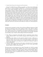
Fig. 1 Schematic model of the human visual system

Let us briefly look at how videos are processed by the human visual system
(HVS) in order to better understand some key concepts of algorithms that we shall
discuss here. Note that even though there have been significant strides in understanding motion processing in the visual cortex, a complete understanding is still
a long way off. What we mention here are some properties which have been confirmed by psycho-visual research. The reader is referred to [10] for a more detailed
explanation of these ideas.
Figure 1 shows a schematic model of the HVS. The visual stimulus in the form
of light from the environment passes through the optics of the eye and is imaged on
the retina. Due to inherent imperfections in the eye, the image formed is blurred,
which can be modeled by a point spread function (PSF) [11]. Most of the information encoded in the retina is transmitted via the optic nerve to the lateral geneiculate
nucleus (LGN). The neurons in the LGN then relay this information to the primary
visual cortex area (V1). From V1, this information is passed on to a variety of visual
areas, including the middle-temporal (MT) or V5 region. V1 neurons have receptive fields1 which demonstrate a substantial degree of selectivity to size (spatial
frequency), orientation and direction of motion of retinal stimulation. It is hypothesized that the MT/V5 region plays a significant role in motion processing [12]. Area
MT/V5 also plays a role in the guidance of some eye movements, segmentation and
3-D structure computation [14], which are properties of human vision that play an
important role in visual perception of videos Unfortunately, as we move from the
optics towards V1 and MT/V5, the amount of information we have about the functioning of these regions decreases. The functioning of area MT is an area of active
research [15].
1

The receptive field of a neuron is its response to visual stimuli, which may depend on spatial
frequency, movement, disparity or other properties. As used here, the receptive field response may
be viewed as synonymous with the signal processing term impulse response.


142

A.K. Moorthy et al.

In this chapter we first describe some HVS-based approaches which try to model
the visual processing stream described above, since these approaches were originally used to predict visual quality. We then describe recently proposed structural
and information-theoretic approaches and feature-based approaches which are commonly used. Further, we describe recent motion-modeling based approaches, and
detail performance evaluation and validation techniques for VQA algorithms. Finally, we touch upon some possible future directions for research on VQA and
conclude the chapter.

HVS – Based Approaches
Much of the initial development in VQA centered on explicit modeling of the HVS.
The visual pathway is modeled using a computational model of the HVS; the original and distorted videos are passed through this model. The visual quality is then
defined as an error measure between the outputs produced by the model for the
original and distorted videos. Many HVS based VQA models are derived from their
IQA counterparts. Some of the popular HVS-based models for IQA include the Visible Differences Predictor (VDP) developed by Daly [16], the Sarnoff JND vision
model [17], the Safranek-Johnston Perceptual Image Coder (PIC) [18] and Watson’s
DCTune [19]. The interested reader is directed to [20] for a detailed description of
these models.
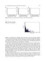
A block diagram of a generic HVS based VQA system is shown in Figure 2.
The only difference between this VQA system and a HVS-based IQA system is the
presence of a ‘temporal filter’. This temporal filter is generally used to model the
two kinds of temporal mechanisms present in early stages of processing in the visual
cortex. Lowpass and bandpass filters have typically been used for this purpose.

The Moving Pictures Quality Metric (MPQM), an early approach to VQA, utilized a Gabor filterbank in the spatial frequency domain, and one lowpass and one
bandpass temporal filter [21]. The Perceptual Distortion Metric [22] was a modification of MPQM and used two infinite impulse response (IIR) filters to model the
lowpass and bandpass mechanisms. Further, the Gabor filterbank was replaced by a
steerable pyramid decomposition [23]. Watson proposed the Digital Video Quality
(DVQ) metric in [24], which used the Discrete Cosine Transform (DCT) and utilized
a simple IIR filter implementation to represent the temporal mechanism. A scalable
wavelet based video distortion metric was proposed in [25]. In this section we describe DVQ and the scalable wavelet-based distortion metric in some detail.

Reference
& test
videos

PreProcessing

Temporal
Filtering

Linear
Transform

Masking
Adjustment

Fig. 2 Block diagram of a generic HVS-based VQA system

Error
Normalization
& Pooling

Spatial

quality
map or
score


6 Digital Video Quality Assessment Algorithms

143

Digital Video Quality Metric
Digital Video Quality Metric (DVQ) metric computes the visibility of artifacts
expressed in the DCT domain. In order to evaluate human visual thresholds on dynamic DCT noise a small study with three subjects was carried out for different
DCT (spatial) and temporal frequencies. The data obtained led to a separable model
which is a product of a temporal, a spatial and an orientation function coupled with
a global threshold.
DVQ metric first transforms the reference and test videos into YOZ color space
[26] and undertakes sampling and cropping. The videos are then transformed using
an 8 8 DCT, then further transformed to local contrast – expressed as the ratio of
DCT amplitude to (filtered) DC amplitude for each block. In the next stage is that of
temporal filtering where a second order IIR filter is used. The local contrast terms are
converted into units of just-noticeable-differences (JNDs) using spatial thresholds
derived from the study followed by contrast masking. Finally, a simple Minkowski
formulation is used to pool the local error scores into the final error score (and hence
the quality score).

Scalable Wavelet-Based Distortion Metric
The distortion metric proposed in [25] can be used as an FR or RR metric depending
upon the application. Further, it differs from other HVS-based metrics in that the
parametrization is performed using human responses to natural videos rather than
sinusoidal gratings.

The metric uses only the Y channel from the YUV color space for processing.
We note that this is true of many of the metrics described in this chapter. Color
and its effect on quality is another interesting area of research [27]. The reference
and distorted video sequences are temporally filtered using a finite impulse response
(FIR) lowpass filter. Then, a spatial frequency decomposition using an integer implementation of a Haar wavelet transform is performed and a subset of coefficients is
selected for distortion measurement. Further, a contrast computation and weighting
by a contrast sensitivity function (CSF) is performed, followed by a masking computation. Finally, following a summation of the differences in the decompositions
for the reference and distorted videos a quality score computation is undertaken.
A detailed explanation of the algorithm and parameter selection along with certain
applications may be found in [25].
In this section we explained only two of the many HVS models. Several HVSbased models have been implemented in commercial products. The reader is directed to [28] for a short description.


144

A.K. Moorthy et al.

Structural and Information-Theoretic approaches
In this section we describe two recent VQA paradigms that are an alternative to
HVS-based approaches – the structural similarity index and the video visual information fidelity. These approaches take into account certain properties of the HVS
when approaching the VQA problem. Performance evaluation of these algorithms
has shown that they perform well in terms of their correlation with human perception. This coupled with the simplicity of implementation of these algorithms makes
them attractive.

Structural Similarity Index
The Structural SIMilarity Index (SSIM) was originally proposed as an IQA algorithm in [29]. In fact, SSIM builds upon the concepts of the Universal Quality Index
(UQI) proposed previously [30]. The SSIM index proposed in [29] is a single-scale
index i.e., the index is evaluated only at the image resolution (and we shall refer
to it as SS-SSIM). In order to better evaluate quality over multiple resolutions, the
multi-scale SSIM (MS-SSIM) index was proposed in [31]. SS-SSIM and MS-SSIM

are space-domain indices. A related index was developed in the complex wavelet
domain in [32] (see also [33]).
Given two image patches x and y drawn from the same location in the reference
and distorted images respectively, SS-SSIM evaluates the following three terms:
luminance l.x; y/, structure s.x; y/, and contrast c.x; y/ as:
l .x; y/ D

2

x

y C C1
2 CC
1
y

2
x

C

2

x y

C C2
C
C C2
C C3
xy

s .x; y/ D
x y C C3
c .x; y/ D

2
x

2
y

and the final SSIM index is given as the product of the three terms:
SSIM .x; y/ D

2
2
x

C

x

y
2
y

C C1

C C1

where,

y are the means of x and y;
are the variances of x and y;
xy is the covariance between x and y; and
C1 , C2 , and C3 D C2 =2 are constants.
x and
2
2
x, y,

2

xy

2
x

C

C C2
2
y

C C2

:


6 Digital Video Quality Assessment Algorithms

145

SS-SSIM computation is performed using a window-based approach, where the
means, standard deviations and cross-correlation are computed within an 11 11
Gaussian window. Thus SS-SSIM provides a matrix of values of approximately the
size of the image representing local quality at each location. The final score for
SSIM is typically computed as the mean of the local scores, yielding a single quality score for the test image. However, other pooling strategies have been proposed
[34], [35]. Note that SSIM is symmetric, attaining the upper limit of 1 if and only
if the two images being compared are exactly the same. Hence, a value of 1 corresponds to perfect quality, and any value lesser than one corresponds to distortion in
the test image. MS-SSIM evaluates structure and contrast over multiple-scales, then
combines them along with luminance, which is evaluated at the finest scale [31].
Henceforth, the acronym SSIM applies to both SS-SSIM and MS-SSIM, unless it is
necessary to differentiate between them.
For VQA, SSIM may be applied on a frame-by-frame basis and the final quality
score is computed as the mean value across frames. Again, this pooling does not
take into account unequal distribution of fixations across the video or the fact that
motion is an integral part of VQA. Hence, in [36], an alternative pooling based on
a weighted sum of local SSIM scores was proposed, where the weights depended
upon the average luminance of the patch and on the global motion. The hypotheses
were - 1) regions of lower luminance do not attract many fixations and hence these
regions should be weighted with a lower value; and 2) high global motion reduces
the perceivability of distortions and hence SSIM scores from these frames should
be assigned lower weights. A block-based motion estimation procedure was used to
compute global motion. It was shown that SS-SSIM performs extremely well on the
VQEG dataset (see section on performance evaluation).

Video Visual Information Fidelity
Natural scene statistics (NSS) have been an active area of research in the recent
past – see [37], [38] for comprehensive reviews. Natural scenes are a small subset
of the space of all possible visual stimuli, and NSS deals with a statistical characterization of such scenes. Video visual information fidelity (Video VIF) proposed in
[39] is based on the hypothesis that when such natural scenes are passed through a

processing system, the system causes a change in the statistical properties of these
natural scenes, rendering them un-natural; and has evolved from VIF used for IQA
[40] (see also [41]). If one could measure this ‘un-naturalness’ one would be able
to predict the quality of the image/video. It has been hypothesized that the visual
stimuli from the natural environment drove the HVS and hence modeling NSS and
HVS may be viewed as dual problems [40]. As mentioned in the introduction, even
though great strides have been made in understanding the HVS, a comprehensive
model is lacking, and NSS may offer an opportunity to fill this gap. Previously,
NSS has been used successfully for image compression [42], texture analysis and
synthesis [43], image denoising [44] and so on.


146

A.K. Moorthy et al.

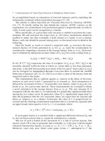
Fig. 3 The model of HVS
for Vide VIF. The channel
introduces distortions in the
video sequence, which along
with the references signal is
received by cognitive processes in the brain

C

Source

Channel

Reference

Test
HVS

E
Receiver

HVS
F
Receiver

It has been shown that the distribution of the (marginal) coefficients of a multiscale, multi-orientation decomposition of a natural image (loosely, a wavelet transform) are heavily peaked at zero, exhibit heavy tails and are well modeled using a
first order Laplacian distribution though they are not independent (but may be approximately second-order uncorrelated). These marginals are well-modeled using
Gaussian scale mixtures (GSM) [45], [46], though other models have been proposed [37].
An extension of VID to video, video VIF, models the original video as a
stochastic source which passes through the HVS, and the distorted video as having
additionally passed through a channel which introduces the distortion (blur, blocking etc.) before passing through the HVS (see Figure 3). Derivatives of the video are
computed and modeled locally using the GSM model [39].
The output of each spatio-temporal derivative (channel) of the original signal is
expressed as a product of two random fields (RF) [45] - a RF of positive scalars and a
zero mean Gaussian vector RF. The channels of the distorted signal are modeled as:
D D GC C V
where, C is the RF from a channel in the original signal, G is a deterministic scalar
field and V is a stationary additive zero-mean Gaussian RF with a diagonal covariance matrix. This distortion model expresses noise by the noise RF V and blur by
the scalar-attenuation field G. The uncertainties in the HVS are represented using
a visual noise term which is modeled as a zero-mean multi-variate Gaussian RF
(N and N 0 ), whose covariance matrix is diagonal. Then define:
E DC CN
F D D C N0
VIF then computes mutual informations between C and E and between C and F ,

both conditioned on the underlying scalar field S. Finally, VIF is expressed as a
ratio of the two mutual informations summed over all the channels.


6 Digital Video Quality Assessment Algorithms

P

147

j 2channels

I.C j I F j js j /

j 2channels

I.C j I E j js j /

VIF D P

where, C j ; F j ; E j ; s j define coefficients from one channel.

Feature Based Approaches
Feature based approaches extract features and statistics from the reference sequences and compare these features to predict visual quality. This definition applies
equally to SSIM and VIF described earlier, however, as we shall see, feature based
approaches utilize multiple features, and are generally not based on any particular
premise such as structural retention or NSS.
Swisscom/KPN research developed the Perceptual Video Quality Metric
(PVQM) [47], which measures three parameters – edginess indicator, temporal
indicator and chrominance indicator. Edginess is compared by using local gradients of luminance of the reference and distorted videos. The temporal indicator

uses normalized cross-correlation between adjacent frames of reference videos.
The chrominance indicator accounts for perceived difference in color information
between the reference and distorted videos. These scores are then mapped onto a
video quality scores. Perceptual Evaluation of Video Quality (PEVQ) from Opticom
was based on the model used in PVQM [48]-[50]. A recent performance evaluation
contest was conducted by the ITU-T for standardization of VQA algorithms [51]
and the ITU-T approved and standardized four full reference VQA algorithms including PVEQ [52]. Another algorithm that uses a feature based approach to VQA
is the Video Quality Metric [53].

Video Quality Metric
Proposed by the National Telecommunications and Information Administration
(NTIA) and standardized by the American National Standards Institute (ANSI),
Video Quality Metric (VQM) [53] was the top performer in the Video Quality Experts Group (VQEG) Phase-II study [54]. The International Telecommunications
Union (ITU) has included VQM as a normative measure for digital cable television
systems [55].
VQM applies a series of filtering operations over a spatio-temporal block which
spans a certain number of rows, columns and frames of the video sequence to extract
seven parameters:
1. a parameter which detects the loss of spatial information, which is essentially an
edge detector, applied on the luminance;
2. a parameter which detects the shift of edges from horizontal and vertical orientation to diagonal orientation, applied on the luminance;


148

A.K. Moorthy et al.

3. a parameter which detects the shift of diagonal edges to horizontal and vertical
orientation, applied on the luminance;
4. a parameter which computes the changes in the spread of the chrominance components;

5. a quality improvement parameter, which accounts for any improvements arising
from sharpening operations;
6. a parameter which is the product of a simple motion detection (absolute difference between frames) and contrast and finally,
7. a parameter to detect severe color impairments.
Each of the above mentioned parameters is thresholded in order to specifically account only for those distortions which are perceptible, then pooled using different
techniques. The general model for VQM then computes a weighted sum of these
parameters to find a final quality index. For VQM, a score of 1 indicates poor quality, while 0 indicates perfect quality. A MATLAB implementation of VQM has been
made available for research purposes online [56].

Motion Modeling Based Approaches
Distortions in a video can either be spatial – blocking artifacts, ringing distortions,
mosaic patterns, false contouring and so on, or temporal – ghosting, motion blocking, motion compensation mismatches, mosquito effect, jerkiness, smearing and so
on [57]. The VQA algorithms discussed so far mainly try to account for loss in
quality due to spatial distortion, but fail to model temporal quality-loss accurately.
For example, the only temporal component of PVQM is a correlation computation
between adjacent frames; VQM uses absolute pixel-by-pixel differences between
adjacent frames of a video sequence.
The human eye is very sensitive to motion and can accurately judge the velocity
and direction of motion of objects in a scene. The ability to detect motion is essential
for survival and for performance of tasks such as navigation, detecting and avoiding
danger and so on. It is hence no surprise that spatio-temporal aspects of human
vision are affected by motion.
As we discussed earlier, initial processing of visual data in the human brain takes
place in the V1 region. Neurons in this front-end (comprising of the retina, LGN
and V1) are tuned to specific orientations and spatial frequencies and are wellmodeled by separable, linear, spatial and temporal filters. Many HVS-based VQA
algorithms use such filters to model this area of visual processing. However, the
visual data from area V1 is transported to area MT/V5 which integrates local motion information from V1 into global percepts of motion of complex patterns [58].
Even though responses of neurons in area MT have been studied and some models of motion sensing have been proposed, none of the existing HVS-based systems
incorporate these models in VQA. Further, a large number of neurons in area MT
are known to be directionally selective and hence movement information in a video

sequence may be captured by a linear spatio-temporal decomposition.


6 Digital Video Quality Assessment Algorithms

149

Recently a temporal pooling strategy based on motion information was proposed
for SSIM [59]. We call this algorithm speed-weighted SSIM and explain some of
its features in this section. Note that the original SSIM for VQA [36], used some
temporal weighting using motion information as well.

Speed-Weighted SSIM
Speed-weighted SSIM (SW-SSIM) [59] considers three kinds of motion fields -1)
absolute motion; which is the absolute pixel motion between two adjacent frames, 2)
background/global motion; which is caused by movement of the image acquisition
system and 3) relative motion; which is the difference between the absolute and
global motion.
It is hypothesized that the HVS is an efficient extractor of information [38].
Visual perception is modeled as an information communication process, where the
HVS is the error prone communication channel since the HVS does not perceive all
information with the same degree of certainty. A psychophysical study conducted
by Stocker and Simoncelli on human visual speed perception suggested that the
internal noise of human speed perception is proportional to the true stimulus speed
[60]. It was found that for a given stimulus speed, a log-normal distribution provides
a good description of the likelihood function (internal noise), which determines the
perceptual uncertainty.
SW-SSIM proceeds as follows. First a SS-SSIM map is constructed at each pixel
location using SSIM as defined before. Then a motion vector field is computed using
Black and Anandan’s multi-scale optical flow estimation algorithm [61] - yielding

absolute pixel motion. Then, a histogram of the motion vectors in each frame is
computed and the vector associated with the peak value is identified as the global
vector for that frame. Relative motion computation follows. The weight applied
at every pixel is then a function of the relative velocity, the global velocity and
the stimulus contrast. The weight is designed such that the importance of a visual
event increases with information content and decreases with perceptual uncertainty.
Finally, each pixel location is weighted and the scores so obtained for each frame is
pooled within and across frames to give a quality index for the video. Note that in
this brief explanation, we have skipped over some practical implementation issues;
the interested reader is directed to [60] for a thorough description of the algorithm.
SW-SSIM was shown to perform well on the VQEG dataset.
Even though SW-SSIM takes into account motion information, only a weighting
of spatially-obtained SSIM scores is undertaken based on this information. We believe that computation of temporal quality of a video sequence is as important, if
not more, as spatial quality computation. Recently, a new VQA algorithm - motion
based video integrity evaluation - that explicitly accounts for temporal quality artifacts was proposed [62], [63].


150

A.K. Moorthy et al.

Motion Based Video Integrity Evaluation
Motion based video integrity evaluation (MOVIE) evaluates the quality of videos
sequences not only in space and time, but also in space-time, by evaluating motion
quality along motion trajectories.
First, both the reference and the distorted video sequences are spatio-temporally
filtered using a family of bandpass Gabor filters. Gabor filters have been used for
motion estimation in video [64], [65] and for models of human visual motion sensing [66]-[68]. It has also been shown that Gabor filters can be used to model the
receptive field of neurons in the visual cortex [69]. Additionally, Gabor filters attain
the theoretical lower bound on uncertainty in the frequency and spatial variables.

MOVIE uses three scales of Gabor filters. A Gaussian filter is included at the center
of the Gabor structure to capture low frequencies in the signal.
A local quality computation of the band-pass filtered outputs of the reference and
test videos is then undertaken by considering a set of coefficients within a window
from each of the Gabor sub-bands. The computation involves the use of a mutual
masking function [70]. The mutual masking is used to model the contrast making
property of the HVS, which refers to a reduction in the visibility of a signal component due to the presence of another spatial component of the same frequency
and orientation in a local neighborhood. This masking model is closely related to
the MS-SSIM and information theoretic models for IQA [71]. The quality index
so obtained is termed as the spatial MOVIE index – even though it captures some
temporal distortions.
MOVIE uses the same filter bank to compute motion information i.e., estimate
optical flow from the reference video. The algorithm used is a multi-scale extension of the Fleet and Jepson [64] algorithm that uses the phase of the complex Gabor
outputs for motion estimation.
Translational motion as an easily accessible interpretation in the frequency
domain : spatial frequencies in the video signal are sheared due to translational
motion along the temporal frequency dimension without affecting the magnitude of
the spatial frequencies and such a translating patch lies entirely within a plane in the
frequency domain [72] The optical flow computation provides an estimation of the
local orientation of this spectral plane at each pixel. Thus, if the motion of the distorted video matches that of the reference video exactly, then the filters that lie along
the motion plane orientation defined by the flow from the reference will be activated
by the distorted video and outputs of filters that lie far away from this plane will be
negligible. In presence of a temporal artifact, however, the motion in the reference
and distorted videos do not match and a different set of filter banks may be activated. Thus, motion vectors from the reference are used to construct velocity-tuned
responses. This can be accomplished by a weighted sum of the Gabor responses,
where positive excitatory weights are assigned to those filters that lie close to the
spectral plane and negative inhibitory weights are assigned to those that lie farther
away from the spectral plane. This excitatory-inhibitory weighting results in a strong
response when the distorted video has motion equal to the reference and a weak response when there is a deviation from the reference motion. Finally, the mean square

6 Digital Video Quality Assessment Algorithms

151

error is computed between the response vectors from the reference video (tuned to
its own motion) and those from the distorted video. The temporal MOVIE index just
described essentially captures temporal quality.
Application of MOVIE to videos produces a map of spatial and temporal scores
at each pixel location for each frame of the video sequence. In order to pool the
scores to create a single quality index for the video sequence, MOVIE uses the
coefficient of variation [73]. Although many alternate pooling strategies have been
proposed [16], [17], [35], [36], [53] the coefficient of variation serves to capture
the distribution of the distortions accurately [74]. The coefficient of variation is
computed for the spatial and temporal MOVIE scores for each frame, then the values
are averaged across frames to create the spatial and temporal MOVIE indices for
the video sequence (temporal MOVIE index uses the square root of the average).
The final MOVIE score is a product of the temporal and spatial MOVIE scores. A
detailed description of the algorithm can be found in [74].

Performance Evaluation & Validation
Practical deployment of the various VQA algorithms discussed previously requires
that a mutually agreed upon testing strategy for evaluation of performance exist. It
was in order to create such a test-bed for the VQA algorithms that the VQEG FRTV phase-I [51] was conducted. A total of 320 distorted video sequences were used
in order to test the performance of 10 leading VQA algorithms, along with PSNR.
The study found that all of the tested algorithms were statistically indistinguishable
from PSNR [51]!.
The test procedure employed by the VQEG was as follows: All of the algorithms were run on the entire database, and then the performance was gauged
based on three criterion : prediction monotonicity, prediction accuracy and prediction consistency. The monotonicity was measured by computing the Spearman
Rank Ordered Correlation Coefficient (SROCC), the accuracy was computed using Linear (Pearson’s) Correlation Coefficient (CC) and Root Mean Square Error

(RMSE). While the SROCC can be computed directly on the scores obtained from
the algorithm and subjective testing, the CC and RMSE require a non-linear transformation before their computation. This is due to the fact that the objective scores
may be non-linearly related to the subjective scores. This would imply that, although
the algorithms predict the quality accurately, in the absence of such a non-linear
mapping the CC and RMSE would not be truly representative of algorithm performance. Finally, consistency was measured by computing the Outlier Ratio (OR).
The standard procedure to conduct a subjective study in order to obtain the mean
opinion scores (MOS) which is representative of the human perception of quality is
enlisted in [3]. A similar study to assess the quality of images was conducted soon
after [75], where leading IQA algorithms were evaluated in a procedure similar to
that followed by the VQEG. The VQEG dataset and the LIVE image dataset are
available publicly at [51] and [76].


152

A.K. Moorthy et al.
Table 1 Performance of VQA algorithms on VQEG
phase-I dataset
VQA Algorithm
SROCC
LCC
PSNR
0.786
0.779
Proponent P8 (Swisscom)[47]
0.803
0.827
Frame-SS-SSIM [36]
0.812
0.849

MOVIE [62]
0.833
0.821

In order to obtain a comparison of the results of various VQA algorithms, in
Table 1 we detail the performance of PVQM [47], which was the top performer in
the VQEG dataset, along with Frame-SS-SSIM and MOVIE. We also include Peak
Signal-to-Noise Ratio (PSNR), since it provides the baseline for performance evaluation, as it has been argued the PSNR does not correlate well with human perception
of quality [77]. Note that many of the algorithms from the VQEG study have been
altered further to enhance performance. Indeed, VQM, whose earlier version was a
proponent in the VQEG study, was trained on the VQEG phase-I dataset in order to
obtain the parameters of the algorithm. We also note that the VQEG phase-I dataset
is the only publicly available dataset for VQA testing.
Although the VQEG dataset has been used in the recent past for performance
evaluation of various VQA algorithms, the dataset suffers from severe drawbacks.
The VQEG dataset contains some non-natural video sequence – eg., scrolling text on
screen – which is not considered ‘fair-game’ for VQA algorithms which are based
on human perception of natural scenes and are not geared towards quality assessment of artificially created environments or text. For example, as demonstrated in
[74], MOVIE performs significantly better when such sequences are not considered
in the analysis. Further, the dataset is dated - the report was published in 2000, and
was made specifically for TV and hence contains interlaced videos. The presence
of interlaced videos complicates the prediction of quality, since the de-interlacing
algorithm can introduce further distortion before computation of algorithm scores.
Further, the VQEG study included distortions only from old generation encoders
such as the H.263 [78] and MPEG-2 [79], which exhibit different distortions compared with present generation encoders like the H.264 AVC/MPEG-4 Part 10 [80].
Finally, and most importantly the VQEG phase I database of distorted videos suffers
from problems with poor perceptual separation. Both humans and algorithms have
difficulty in producing consistent judgments that distinguish many of the videos,
lowering the correlations between humans and algorithms and the statistical confidence of the results. We also note that even though the VQEG has conducted other
studies [54], oddly, none of the data has been made public.

In order to overcome these limitations the LIVE video quality assessment and
the LIVE wireless video quality databases were created. These two databases will
alleviate the problems associated with the VQEG dataset and will provide a suitable
testing ground for future VQA algorithms. Information regarding these databases
may not be ready before this chapter is published, but will soon be provided at [76].


6 Digital Video Quality Assessment Algorithms

153

Conclusions & Future Directions
In this chapter we began by motivating the need for VQA algorithms and gave a
brief summary of various VQA algorithms. We detailed performance evaluation
techniques and validation methods for a number of leading VQA algorithms. Future
research may involve further understanding of human motion processing and its incorporation into VQA algorithms. Temporal pooling is another issue that needs to
be considered. Gaze attention and region-of-interest remain interesting areas of research, especially in the case of video quality assessment. In this chapter we have
detailed only FR VQA algorithms. However, research in the area of RR VQA algorithms is of key interest, considering its practical advantages. The Holy Grail,
of course are truly NR VQA algorithms. Further, the statistical techniques used for
measuring the performance of algorithms have been questioned [35], [75]. It is of
interest to evaluate various possible alternatives to study correlation with human
perception.

References
1. Z. Wang and A. C. Bovik, Modern Image Quality Assessment. New York: Morgan and
Claypool Publishing Co., 2006.
2. A. K. Moorthy and A. C. Bovik, “Perceptually Significant Spatial Pooling techniques for Image quality assessment ,” in SPIE Conference on Human Vision and Electronic Imaging, Jan.
2009.
3. “Methodology for the subjective assessment of the quality of television pictures,” ITU-R Recommendation BT.500-11.
4. B. Hiremath, Q. Li and Z. Wang “Quality-aware video,” IEEE International Conference on

Image Processing, San Antonio, TX, Sept. 16-19, 2007.
5. H. R. Sheikh, A. C. Bovik, and L. Cormack, “No-reference quality assessment using natural
scene statistics: JPEG2000,” Image Processing, IEEE Transactions on, vol. 14, no. 11, pp.
1918–1927, 2005.
6. C. M. Liu, J. Y. Lin, K. G. Wu and C. N. Wang, “Objective image quality measure for blockbased DCT coding,” IEEE Trans. Consum. Electron., vol. 43, pp. 511–516, 1997.
7. Z. Wang, A. C. Bovik, and B. L. Evans, “Blind measurement of blocking artifacts in images,”
in IEEE Intl. Conf. Image Proc, 2000.
8. X. Li, “Blind image quality assessment”, IEEE International Conference on Image Processing,
New York, 2002.
9. Patrick Le Callet, Christian Viard-Gaudin, St´ phane P´ chard and Emilie Caillault, “No refe
e
erence and reduced reference video quality metrics for end to end QoS monitoring”, Special
Issue on multimedia Qos evaluation and management technologies, E89, (2), Pages: 289-296,
February 2006.
10. W. S. Geisler and M. S. Banks, “Visual performance,” in Handbook of Optics, M. Bass, Ed.
McGraw-Hill, 1995.
11. B. A. Wandell, Foundations of Vision. Sunderland, MA: Sinauer Associates Inc., 1995.
12. N. C. Rust, V Mante, E. P. Simoncelli, and J. A. Movshon, “How MT cells analyze the motion
of visual patterns ”, Nature Neuroscience, vol.9(11), pp. 1421–1431, Nov 2006.
13. Z. Wang, G. Wu, H. R. Sheikh, E. P. Simoncelli, E.-H. Yang and A. C. Bovik, ”Quality -aware
images” IEEE Transactions on Image Processing, vol. 15, no. 6, pp. 1680-1689, June 2006.
14. R. T. Born and D. C. Bradley, “Structure and function of visual area MT,” Annual Rev Neuroscience, vol. 28, pp. 157–189, 2005.


154

A.K. Moorthy et al.

15. M. A. Smith, N. J. Majaj, and J. A. Movshon, “Dynamics of motion signaling by neurons in
macaque area MT,” Nature Neuroscience, vol. 8, no. 2, pp. 220–228, Feb. 2005.

16. S. Daly, “The visible differences predictor: an algorithm for the assessment of image fidelity,”
in Digital Images and Human Vision (A. B. Watson, ed.), pp. 179–206, Cambridge, MA: The
MIT Press, 1993.
17. J. Lubin, “The use of psychophysical data and models in the analysis of display system performance,” in Digital Images and Human Vision (A. B. Watson, ed.), pp. 163–178, Cambridge,
MA: The MIT Press, 1993.
18. R. J. Safranek and J. D. Johnston, “A perceptually tuned sub-band image coder with image
dependent quantization and post-quantization data compression,” in Proc. ICASSP-89, vol. 3,
(Glasgow, Scotland), pp. 1945–1948, May 1989.
19. A. B.Watson, “DCTune: a technique for visual optimization of dct quantization matrices for
individual images,” Society for Information Display Digest of Technical Papers, vol. 24, pp.
946–949, 1993.
20. K. Seshadrinathan, R. J. Safranek, J. Chen, T. N. Pappas, H. R. Sheikh, E. P. Simoncelli,
Z. Wang and A. C. Bovik. Image quality assessment. In A. C. Bovik, editor, The Essential
Guide to Image Processing, chapter 20. Academic Press, 2009.
21. C. J. van den Branden Lambrecht and O. Verscheure, “Perceptual quality measure using a
spatiotemporal model of the human visual system,” in Proc. SPIE, vol. 2668, no. 1. San Jose,
CA, USA: SPIE, Mar. 1996, pp. 450–461.
22. S. Winkler, “Perceptual distortion metric for digital color video,” Proc. SPIE, vol. 3644, no.
1, pp. 175–184, May 1999.
23. E. P. Simoncelli, W. T. Freeman, E. H. Adelson, and D. J. Heeger, “Shiftable multiscale transforms,” IEEE Trans. Inform. Theory, vol. 38, pp. 587-607, Mar. 1992.
24. A. B. Watson, J. Hu, and J. F. McGowan III, “Digital video quality metric based on human
vision,” J. Electron. Imaging, vol. 10, no. 1, pp. 20–29, Jan. 2001.
25. M. Masry, S. S. Hemami, and Y. Sermadevi, “A scalable wavelet-based video distortion metric
and applications,” Circuits and Systems for Video Technology, IEEE Transactions on, vol. 16,
no. 2, pp. 260–273, 2006.
26. H. Peterson, A.J. Ahumada, Jr. and A. Watson,”An Improved Detection Model for DCT Coefficient Quantization,” Human Vision and Electronic Imaging, Proc. SPIE, 1913, 191–201.
27. M. Carnec, P. Le Callet, and D. Barba, “Objective quality assessment of color images based
on a generic perceptual reduced reference,” Signal Processing: Image Communication, Volume
23 , Issue 4, Pages 239-256, April 2008.
28. K. Seshadrinathan and A. C. Bovik. Video quality assessment. In A. C. Bovik, editor, The

Essential Guide to Video Processing, chapter 14. Academic Press, 2009.
29. Z. Wang, A. C. Bovik, H. R. Sheikh, and E. P. Simoncelli, “Image quality assessment: from
error visibility to structural similarity,” IEEE Trans. Image Process, vol. 13, no. 4, pp. 600–612,
2004.
30. Z. Wang and A. C. Bovik, “A universal image quality index,” IEEE Signal Processing Letters,
vol. 9, no. 3, pp. 81–84, 2002.
31. Z. Wang, E. P. Simoncelli, and A. C. Bovik, “Multiscale structural similarity for image quality
assessment,” in Thirty-Seventh Asilomar Conf. on Signals, Systems and Computers, Pacific
Grove, CA, 2003.
32. Z. Wang and E. P. Simoncelli, “Translation insensitive image similarity in complex wavelet
domain,” in IEEE Intl. Conf. Acoustics, Speech, and Signal Process., Philadelphia, PA, 2005.
33. M. P. Sampat, Z. Wang, S. Gupta, A. C. Bovik and M. K. Markey, ”Complex wavelet structural
similarity: A new image similarity index,” IEEE Transactions on Image Processing, to appear
2009.
34. Z. Wang and X. Shang, “Spatial pooling strategies for perceptual image quality assessment,”
in IEEE International Conference on Image Processing, Jan. 1996.
35. A. K. Moorthy and A. C. Bovik, “Visual importance pooling for image quality assessment,”
IEEE Journal of Selected Topics in Signal Processing, Special Issue on Visual Media Quality
Assessment, to appear, April 2009.


6 Digital Video Quality Assessment Algorithms

155

36. Z. Wang, L. Lu, and A. C. Bovik, “Video quality assessment based on structural distortion
measurement,” Signal Processing: Image Communication, vol. 19, no. 2, pp. 121–132, Feb.
2004.
37. A. Srivastava, A. B. Lee, E. P. Simoncelli, and S.-C. Zhu, “On advances in statistical modeling
of natural images,” J. Math. Imag. Vis., vol. 18, pp. 17–33, 2003.

38. E. P. Simoncelli and B. A. Olshausen, “Natural image statistics and neural representation,”
Annu. Rev. Neurosci., vol. 24, pp. 1193–1216, May 2001.
39. H. R. Sheikh and A. C. Bovik, “A visual information fidelity approach to video quality assessment,” First International Workshop on Video Processing and Quality Metrics for Conusmer
Electronics, Jan. 2005.
40. H. R. Sheikh and A. C. Bovik, “Image information and visual quality,” IEEE Trans. Image
Process, vol. 15, no. 2, pp. 430-444, 2006.
41. H. R. Sheikh, A. C. Bovik, and G. de Veciana, “An information fidelity criterion for image
quality assessment using natural scene statistics,” IEEE Trans. Image Process., vol. 14, no. 12,
pp. 2117-2128, 2005.
42. J. Malo, I. Epifanio, R. Navarro, and E. P. Simoncelli, “Non-linear image representation for
efficient perceptual coding”, IEEE Transactions on Image Processing, vol.15(1), pp. 68–80,
Jan 2006.
43. J. Portilla and E. P. Simoncelli, “ A parametric texture model based on joint statistics of complex wavelet coefficients”, International Journal of Computer Vision, vol.40(1), pp. 49–71,
Dec 2000.
44. J. A. Guerrero-Col´ n, E. P. Simoncelli , and J. Portilla, “Image denoising using mixtures of
o
Gaussian scale mixtures “, IEEE International Conference on Image Processing, pp. 565–568,
Oct 2008.
45. M. J. Wainwright, E. P. Simoncelli, and A. S. Wilsky, “Random cascades on wavelet trees and
their use in analyzing and modeling natural images,” Applied and Computational Harmonic
Analysis, vol. 11, pp. 89–123, 2001.
46. M. J. Wainwright and E. P. Simoncelli, “Scale Mixtures of Gaussians and the statistics of
natural images”, Adv. Neural Information Processing Systems (NIPS’99), vol.12 pp. 855–861,
May 2000.
47. A. P. Hekstra, J. G. Beerends, D. Ledermann, F. E. de Caluwe, S. Kohler, R. H. Koenen, S.
Rihs, M. Ehrsam, and D. Schlauss, “PVQM - A perceptual video quality measure,” Signal
Proc.: Image Comm. vol. 17, pp. 781–798, 2002.
48. Opticom. [Online]. Available: />49. M. Malkowski and D. Claben, “Performance of video telephony services in UMTS using live
measurements and network emulation,” Wireless Personal Comm., vol. 1, pp. 19–32, 2008.
50. M. Barkowsky, J. Bialkowski, R. Bitto, and A. Kaup, “Temporal registration using 3D phase

correlation and a maximum likelihood approach in the perceptual evaluation of video quality,”
in IEEE Workshop on Multimedia Signal Proc., 2007.
51. The Video Quality Experts Group. (2000) Final report from the video quality experts group on
the validation of objective quality metrics for video quality assessment. [Online]. Available:
phaseI
52. Objective perceptual multimedia video quality measurement in the presence of a full reference,
International Telecommunications Union Std. ITU-T Rec. J. 247, 2008.
53. M. H. Pinson and S. Wolf, “A new standardized method for objectively measuring video quality,” IEEE Trans. Broadcast., vol. 50, no. 3, pp. 312–322, Sep. 2004.
54. The Video Quality Experts Group. (2003) Final VQEG report on the validation of
objective models of video quality assessment. [Online]. Available: . bldrdoc.gov/vqeg/projects/frtv phaseII
55. Objective perceptual video quality measurement techniques for digital cable television in the
presence of a full reference, International Telecommunications Union Std. ITU-T Rec. J. 144,
2004.


156

A.K. Moorthy et al.

56. “Video quality metric.” [Online]. Available: software.php
57. M. Yuen and H. R. Wu, “A survey of hybrid MC/DPCM/DCT video coding distortions,” Signal
Processing, vol. 70, no. 3, pp. 247–278, Nov. 1998.
58. J. A. Movshon and W. T. Newsome, “Visual response properties of striate cortical neurons
projecting to Area MT in macaque monkeys,” J. Neurosci., vol. 16, no. 23, pp. 7733–7741,
1996.
59. Z.Wang and Q. Li, “Video quality assessment using a statistical model of human visual speed
perception.” J Opt Soc Am A Opt Image Sci Vis, vol. 24, no. 12, pp. B61–B69, Dec 2007.
60. A. A. Stocker and E. P. Simoncelli, “Noise characteristics and prior expectations in human
visual speed perception,” Nature Neuroscience, 9, 578-585 (2006).
61. Black, M. J. and Anandan, P., “The robust estimation of multiple motions: Parametric and

piecewise-smooth flow fields,” Computer Vision and Image Understanding, 63, 75-104 (1996).
62. K. Seshadrinathan and A. C. Bovik, “Spatio-temporal quality assessment of natural videos,”
IEEE Transactions on Image Processing, submitted for publication.
63. K. Seshadrinathan and A. C. Bovik, “A structural similarity metric for video based on motion
models,” IEEE International Conference on Acoustics, Speech, and Signal Processing, 2007.
64. D. J. Fleet and A. D. Jepson, “Computation of component image velocity from local phase
information,” International Journal of Computer Vision, vol. 5, no. 1, pp. 77–104, 1990.
65. D. J. Heeger, “Optical flow using spatiotemporal filters,” International Journal of Computer
Vision, vol. 1, no. 4, pp. 279–302, 1987.
66. E. H. Adelson and J. R. Bergen, “Spatiotemporal energy models for the perception of motion.”
J Opt Soc Am A, vol. 2, no. 2, pp. 284–299, Feb 1985.
67. N. J. Priebe, S. G. Lisberger, and J. A. Movshon, “Tuning for spatiotemporal frequency and
speed in directionally selective neurons of macaque striate cortex.” J Neurosci, vol. 26, no. 11,
pp. 2941–2950, Mar 2006.
68. E. P. Simoncelli and D. J. Heeger, “A model of neuronal responses in visual area MT,” Vision
Res, vol. 38, no. 5, pp. 743–761, Mar 1998.
69. J. G. Daugman, “Uncertainty relation for resolution in space, spatial frequency, and orientation optimized by two-dimensional visual cortical filters,” Journal of the Optical Society of
America A (Optics and Image Science), vol. 2, no. 7, pp. 1160–1169, 1985.
70. P. C. Teo and D. J. Heeger, “Perceptual image distortion,” in Proceedings of the IEEE International Conference on Image Processing. IEEE, 1994, pp. 982–986 vol.2.
71. K. Seshadrinathan and A. C. Bovik, “Unifying analysis of full reference image quality assessment,” in IEEE Intl. Conf. on Image Proc., 2008.
72. A. B. Watson and J. Ahumada, A. J., “Model of human visual-motion sensing,” Journal of the
Optical Society of America A (Optics and Image Science), vol. 2, no. 2, pp. 322–342, 1985.
73. H. Frank and S. C. Althoen, “The coefficient of variation,” in Statistics: Concepts and Applications. Cambridge, Great Britan: Cambridge University Press., 1995, pp. 58–59.
74. K. Seshadrinathan, “Video quality assessment based on motion models,” Ph.D. dissertation,
University of Texas at Austin, 2008.
75. H. R. Sheikh, M. F. Sabir, and A. C. Bovik, “A statistical evaluation of recent full reference
image quality assessment algorithms,” IEEE Transactions on Image Processing, vol. 15, no.
11, pp. 3440–3451, Nov. 2006.
76. LIVE image quality assessment database. [Online]. Available: xas.
edu/research/quality/subjective.html

77. Wang, Z. and Bovik, A. C., “Mean squared error: Love it or leave it? - a new look at fidelity
measures.” IEEE Signal Processing Magazine. January 2009.
78. “Video coding for low bit rate communication”, ITU Recommendation H.263.
79. “Generic coding of moving pictures and associated audio information - part 2: Video,” 1994,
ITU-T and ISO/IEC JTC 1. ITU-T Recommendation H.262 and ISO/IEC 13 818-2 (MPEG-2).
80. “Advanced video coding,” 2003, ISO/IEC 14496-10 and ITU-T Rec. H.264.


Chapter 7

Countermeasures for Time-Cheat Detection
in Multiplayer Online Games
Stefano Ferretti

Introduction
Cheating is an important issue in games. Depending on the system over which the
game is deployed, several types of malicious actions may be accomplished so as
to take an unfair and unexpected advantage over the game and over the (digital,
human) adversaries. When the game is a standalone application, cheats typically
just relate to the specific software code being developed to build the application.
It is not a surprise to find (in the Web and in specialized magazines) people that
explain cheats on specific games stating, for instance, which configuration files can
be altered (and how to do it) to automatically gain some bonus during the game. To
avoid this, game developers are hence motivated to build stable code, with related
data that should be securely managed and made difficult to alter.
When the game goes online, a number of further issues arise which highly complicate the task of avoiding cheats. Indeed, each node in a Multiplayer Online Game
(MOG) has its own, locally installed software, which can be freely altered or substituted by the malicious player. Furthermore, and certainly equally important, the
presence of the network and the need for communication among nodes in a MOG
can be exploited by some of these nodes to cheat.
It is the best-effort nature of the Internet that allows cheaters to take malicious

actions to evade the rules of the game. For instance, they are enabled to alter timing
properties of game events in order to mimic that these have been generated at a certain point in (game) time (these are often referred as time cheats). Cheaters can delay
(or anticipate) the notification of their game events to other nodes in the system.
They can also drop some of their game events (i.e. not notify them to other nodes)
in order to save their own computational and communication resources (sending a
message has a cost) and diminish the amount of updated information provided to
other participants.
S. Ferretti ( )
Department of Computer Science, University of Bologna, Bologna, Italy
e-mail:
B. Furht (ed.), Handbook of Multimedia for Digital Entertainment and Arts,
DOI 10.1007/978-0-387-89024-1 7, c Springer Science+Business Media, LLC 2009

157


158

S. Ferretti

These last classes of cheats must be avoided by devising specific, applicationaware communication protocols. In this manuscript, we will deal with time cheats
and outline two classes of mechanisms to avoid them, i.e. prevention and detection
schemes. We will describe some of the existing approaches in a peer-to-peer (P2P)
system architecture that exploits a specific game time model. The reason behind the
choice of a P2P architecture is that it has been generally recognized as a powerful
solution to guarantee a high level of scalability and fault tolerance in MOGs. The
adopted game time model is a general framework which ensures a fair management
of game events generated at distributed nodes.
In the reminder of this discussion, we will first outline some background on the
system architectures employed to support MOGs. We will explain why P2P solutions are generally a better choice with respect to the client/server model. We then

present the system model exploited to prevent time cheats and countermeasures
to avoid them. A discussion on the framework exploited to model game time advancements is provided in the subsequent section. The idea is that of resorting to a
combination of simulation and wallclock times. Some prominent time cheats, which
have been considered by the research community, are then discussed. Preventions
schemes are explained, focusing on those approaches that prevent the look-ahead
time cheat. The discussion continues with detection schemes, together with some
simulation results that confirm the viability of these approaches. Finally, some concluding remarks are outlined.

Background on System Architectures
MOGs may be deployed on the Internet, based on different distributed architectures
[14]. Besides classical issues concerned with scalability, fault-tolerance and responsiveness, the choice of the architecture to support a MOG is of main importance also
on cheating avoidance. Indeed, different game architectures entail different ways to
manage the game state, different communication protocols among distributed nodes,
different information directly available at (malicious) players. These differences
have strong influence also on the way cheats can be accomplished (and contrasted).
For instance, peer-to-peer based approaches represent very promising architectural solutions [15]. Each peer manages its own copy of the game state, which is
locally updated based on the messages received by other peers. Communication and
synchronization protocols are exploited to be sure that each peer eventually receives
all the game events generated by player, hence being able to compute a correct evolution of the game state. P2P architectures and protocols allow a scalable and fault
tolerant management of a MOG; they enable self-configuring solutions that face the
diverse nature of players’ devices and the underlying network. However, the main
advantage of P2P in MOGs, i.e. the autonomy of peers, may become an issue when
cheaters join the game, since they have a free access to the game state.
Conversely, it is well known that client/server architectures fail to provide scalability, since the server often represents a bottleneck and the single point of failure


7 Countermeasures for Time-Cheat Detection in Multiplayer Online Games

159

in the system. In this case, only the server controls the game state which is updated
based on the messages sent by clients; the server is then responsible for periodically
informing clients about the changes on the game state. This model clearly reduces
the possible cheats in the system (without completely avoiding them).
For the reasons mentioned above, it becomes interesting to study whether effective cheating avoidance schemes can be devised on top of P2P architectures. This
would enable the provision of fault-tolerant, scalable and secure platforms on top of
which games could be played by a multitude of users.

System Model
In the rest of the discussion, we model the game system as composed of several
peers organized as a P2P architecture. We assume that each peer maintains a local
copy of the game state and keeps it synchronized with others managed by distributed
peers, based on notified updates. No assumptions are made here on the exploited
synchronization algorithm to maintain game state consistency. There are several
possible alternatives, such as, just to mention a few, [8, 19, 26, 28]. For the sake of
simplicity, we assume that peers are fully connected, i.e. they can communicate with
other nodes directly, without the need to pass through some other node. Needless to
say, such assumption is made at the application layer (not at the network layer), just
to assert that no overlay network is exploited for the game event dissemination.
We denote with … the set of peers in the P2P game architecture; pi identifies a
single peer, i.e., pi 2 …. With …i we indicate all peers but pi , i.e. …i D … fpi g.
Similarly, notations such as …i;j indicate all peers but pi and pj , i.e. …i;j D …
˚
«
pi ; pj .
To characterize game events produced at a given peer (i.e. by the same player)
we employ an identifier with prime notations, i.e. e i is an event generated by pi .
Instead, to identify and order events generated (often by the same peer) in different
time instants, we employ subscripts, e.g. ej , ek , j < k. Figure 1 provides a graphical
view of the system model, with the associated notation, when only three peers, i.e.

p1 , p2 , p3 , constitute the architecture. In the Figure, a game event e 1 is generated
and sent from p1 to p2 . Also the sets … and …1 are represented.
Game events are notified within messages. Typically, MOGs exploit UDP-based
delivery solutions to transmit game events [28]. However, for the sake of simplicity,

p1

δ12 = δ21

δ13= δ31

Fig. 1 System model

e1

p3

δ12(e1)
p2

δ23= δ32

Π = {p1, p2, p3}
Π1 ={p2, p3}


160

S. Ferretti

in our scheme we will assume that transmitted messages can experience different
latencies and delay jitters but cannot be lost. We assume the existence of an upper
bound UB on the latencies among peers in the system. UB is known by peers. With
•ij .e/ we denote the time needed to transmit a game event e from pi to pj . (In
Figure 1, the time to send e1 from p1 to p2 is characterized as •12 e 1 .) With •ij ,
instead, we denote the average latency needed for the transmission of a non specified
game event from pi to pj . We realistically assume that typically •ij .e/
•ij .
Basically, this last assumption entails that the underlying network over which the
game is deployed offers a best-effort service with unpredictable delay latencies and
jitters but, on the long run, an average trend of network latencies may be observed.
This is in accordance with a plethora of works that model network traffic such as,
in the networked gaming literature, [3, 13, 23]. We also assume that transmission
latencies are mostly symmetric, i.e. •ij D •j i (as shown in Figure 1).

Modeling Game Time
Games evolve through events generated by distributed players during time. Time is
thus a main characteristic to model in a game. Obviously, several possibilities exist.
A first distinction is on who assigns timestamps to the game events. An approach
is to leave to a single node (e.g. the server) the task of timestamping and ordering
game events. This, however, introduces a high level of unfairness, since transmission
latencies to reach that node influence the game event ordering. The other approach
is that peers locally assign timestamps to their own generated game events.
It is worth mentioning that most developed games simply adopt the use of a
single timestamp to manage the game time. This timestamp is obtained based on the
physical clock at the node where the game is executed. However, since the game is
played in multiplayer mode, different physical clocks of different nodes timestamp
different game events. As a consequence, when these events are processed according
to their timestamp order, it is obvious that a fair ordering of game events is obtained
only provided that physical clocks of distributed nodes are perfectly synchronized.

Yet, this assumption is not realistic, especially when a high number of nodes is
involved in the game. Hence, those nodes that have a slow clock are advantaged
with respect to other ones.
Trying to provide a fair way to characterize game events produced at distributed
nodes in a MOG, a main notion worth of introduction is that of simulation time.
Simulation time is the abstraction that is used to model when events have been produced within the virtual game timeline. In the context of distributed simulation,
Fujimoto defined in [21] simulation time as a “set of values where each value
represents an instant of time in the system being modelled”. The simulation time
measured at a peer pi is denoted with S T i . With S T i .e/, we represent the simulation time associated to the game event e, generated by the peer pi .
Wallclock time, instead, is the time that identifies when the game takes place at
a physical node. We denote with W T i the wallclock time measured at pi . W T i .e/


7 Countermeasures for Time-Cheat Detection in Multiplayer Online Games

161

represents the wallclock time of generation of the game event e at pi . We assume
Q
that once created, the transmission of the event e from pi to all other peers i is
instantaneous (unless pi is a cheater). Moreover, we denote with W T j rec .e/ the
wallclock time of reception of e at pj .
As mentioned, simulation time is an important notion to characterize game events
generated by different peers, and then to totally order them. It serves to have a fair
way to inject game events in the game world. However, the use of simulation time
alone could result as a weakness in terms of cheating avoidance. In fact, in principle
each peer is enabled to associate whatever simulation time to its produced game
event.
This problem can be reduced in some way, by exploiting ST together with
WT and keeping simulation time advancements proportional to wallclock ones

(see equation (1) below). A mapping function TiW can hence be introduced that
transforms a simulation time s into the corresponding wallclock time t at pi , i.e.
TiW .s/ D t . With TiS , instead, we represent TiW 0 s inverse function. The specific
game time model will depend on the definition of TiW and TiS .
ST and WT can be employed to divide time in coarse intervals, thus adopting a
round-based game evolution (i.e. at each round a single move per player is allowed),
or mimicking a fluid evolution of time. In particular, in a round-based evolution of
the game, ST advances as a step function of WT. In other words, ST increases of a
s only once all messages from other peers have been received, or a (wallclock)
timeout has expired, i.e. Tis .t C h/ D Tis .t / D s, for h < t , where t is the
minimum between time needed to receive all messages from all peers …i and a
predefined wallclock timeout. After such t, ST advances to s C s.
Conversely, to make the system able to advance in real-time, a function Tis must
be employed to let ST advance in synchrony with WT. A scale factor k may be
exploited to identify the pace of game advancements in the simulated world. When
k D 1, a real-time evolution is implemented; otherwise, i.e. k ¤ 1, the system is
said to advance in scaled real-time [7, 21]. The mapping function to translate WT
into ST is thus
Tis .ti;act ual / D Tis .ti;start / C k.ti;act ual

ti;start /;

(1)

where ti;actual represents the actual WT at pi , ti;start represents the wallclock time
associated to the beginning of the game at pi . The mapping Tis .ti;start / returns a
simulation time value, agreed and shared among all nodes, representing the time at
which the beginning of the game plot takes place, i.e., Tis .ti;start / D sstart 2 S T ,
8 pi 2 …. Using the formula above, the simulation time of a given game event e
can be characterized as follows,

S T i .e/ D sstart C k .W T i .e/

ti;start / :

(2)

The binding between these two different timestamps prevent that simulation times
are freely altered by cheaters without tampering also wallclock times (in order to respect such mapping between ST and WT). Hence, upon reception of cheated events,


162

S. Ferretti

based on contained timestamps, honest peers will measure altered network latencies
which differ from the real ones. This way, viable detection schemes can be devised,
for example, based on statistical methods that measure transmission latencies, as
explained in the rest of the work.
Such an approach to model time advancements allows also to cope with the fact
that physical clocks of nodes in the system are not synchronized and that nodes cannot start the game at the same, precise instant. In fact, due to the distributed nature
of a MOG, with high probability ti;start Ô tj;start , 8pi , pj 2 , i Ô j . A solution here is to let each peer pi to associate, at the beginning of the game session, its
starting wallclock time ti;start to the agreed constant starting simulation time, i.e.
Tis .ti;start / D sstart . Then, each player notifies others with its own ti;start .
An important praxis for an efficient delivery protocol is that of exploiting, at the
beginning of the game a clock synchronization protocol. This can be accomplished
by resorting to an approach that could be devised based on to those presented in literature, e.g. [6, 7, 10, 12, 27]. This would allow to obtain an initial estimation of the
average network latencies among peers •ij and of the drift among physical clocks at
pi and pj (i.e. driftij ). By convention, driftij > 0 if pj reaches a given wallclock
time t before pi (i.e., pj has wallclock times higher than pi , see Figure 2). We assume that the effects of the drift clock rate at all peers are negligible. Based on such
drift, it is easy to characterize the wallclock time at a given peer pj when an event

e i is generated at pi , i.e. W T i e i C driftij . Hence, upon reception of a game event
e from pi to pj , based on the timestamp included in the message pj can measure
ıij .e/ D W Tjrec .e/

W Ti .e/

driftij :

(3)

Of course, such measurement can be considered as a reliable information only provided that driftij is accurately estimated and that pi is not cheating (i.e. pi has not
altered the timestamp in its message).
Also a gap ij may be measured representing the (real) time interval between the
instants at which pi and pj start the game (see Figure 3). A simple equation to
measure gap ij , based on the starting point of the beginning time instant (including
driftij / is as follows,
gapij D driftij C ti;start

tj;start :

(4)

In essence, gap ij takes into account that a drift among clocks of pi and pj exists
and that they started the game at different times. Clearly, gap ij D gap ij (as

t*
pi

WTi
t*

pj

Fig. 2 Drift between pi
and pj

WTj
driftij


7 Countermeasures for Time-Cheat Detection in Multiplayer Online Games
Fig. 3 Gap between pi
and pj

163

ti,star t

pi

WTi
pj

tj,star t
gapij

WTj

well as driftij D driftij ). Methods can be adopted to reduce the value of the gap
among peers. For instance, an agreement protocol could force peers do determine a

certain point in time to start the game session. Alternatively, a peer pl may be set to
broadcast a start message to other ones that begin the game as soon as they receive
that message; for each transmitted message, a buffering delay may be utilized at pl ,
adapted for each receiver to compensate for different network latencies. This way,
the start message is received by all peers within a short time interval.

Time Cheats
Time cheats are those specific cheats which are based on the illegal alteration of
game events’ timestamp. These cheats are distinctive of Internet-based MOGs and
can be profitably exploited by malicious players when the game is hosted on a P2P
platform and each peers locally assigns a timestamp to each generated game event
[4, 5, 16–18]. The alibi of cheaters is the variable transmission latency that a message may experience when it travels on the Internet.
Needless to say, the simpler the model to characterize game time, the simpler is
to alter the communication protocol to gain some malicious advantage. Hence, time
cheats vary and depend also on the game time management protocol. When resorting
to (1) and (2) to model game time, an important implication is that cheaters which
want to alter timing properties of their generated events are forced to alter both ST
and WT. Indeed, the communication protocol may impose that for each transmitted
event e, both S T i .e/ and W T i .e/ are included (together with a sequence number
and other game-related data) within the message transporting e. Thus, given any two
game events e i h and e i l , and based on (2), a check can be made to verify that the
following holds,
i
S Ti eh

W

i
Ti eh

i
S Ti el
i
W Ti el

D k:

(5)

Conversely, it is straightforward to verify that (5) is not respected by pi , which in
this case is a cheater.
In the following, we will define some prominent time cheats presented in the
research literature related to MOGs.