Recent Developments of Electrical Drives - Part 46 ppsx

III-3.5. Improved Modeling of Three-Phase Transformer Analysis 453
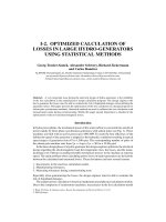
Figure 2. Calculated Fourier series curve and measured curve.
The calculated Fourier series curve and the measured curve are illustrated in Fig. 2. The
Fourier coefficients a
k
are computed once, then stored for the determination of B = f (H)
or U = f (I) for all possible values of H or I. The measured curve considered in this study
corresponds to the line-to-line voltage in the primary, and to the current of the phase A of
the primary winding.
Numerical approach
Two methods have been developed for this approach. For both methods, the leakage in-
ductances L
σ 1
, L
σ 2
of the primary and secondary windings, as well as the zero-sequence
inductances L
01
, L
02
are considered as constants. The first one considers the total magnetic
flux as state variables. The corresponding set of six differential equations is given by:
d[ψ]
dt
= [B] (7)
[B] =

u
ABC
− R
ABC

·i
ABC
u
abc
− R
abc
·i
abc

(8)
where R
ABC
is the resistances of the primary windings and R
abc
is the resistances of the
secondary windings.
The total magnetic flux of different windings, including zero-sequence flux are given by:
[ψ] = [L] · [i] (9)
The self and mutual inductances are expressed in function of the magnetic reluctances
R
1T
, R
2T
, R
3T
of the equivalent magnetic circuit-diagrams, with N
1
, N
2
the turns of the

primary respectively secondary windings. For example, the magnetizing inductance of the
primary winding A respectively the mutual inductance between the primary winding A and
454 Kawkabani and Simond
the secondary one b are given by:
L
h1A
=
N
2
1
R
1T
+
R
2T
· R
3T
R
2T
+ R
3T
=
N
2
1
· (R
2T
+ R
3T
)

R
1T
· R
2T
+ R
1T
· R
3T
+ R
2T
· R
3T
(10)
L
Ab
=
−N
1
· N
2
· R
3T
R
1T
· R
2T
+ R
1T
· R
3T

+ R
2T
· R
3T
(11)
Similar expressions are determined for all the inductances. The determination of the
magnetic flux at each integration step permits to evaluate and adapt, by the B-H curve, the
different magnetic reluctances as well as different inductances.
Some numerical software package like SIMSEN [2] (fl.ch) use essen-
tially the currents as state variables. For this purpose, a second method has been developed.
This one considers the following set of differential equations:
[A] ·
d[X]
dt
= [B] (12)
with:
[B] =
⎡
⎣
u
ABC
− R
ABC
·i
ABC
u
abc
− R
abc
·i

abc
u
ABC
− R
ABC
·i
ABC
⎤
⎦
(13)
[X]
T
=
[
i
A
i
B
i
C
i
a
i
b
i
c
ψ
A
ψ
B

ψ
C
]
In this case, one needs three supplementary state variables ψ
A
, ψ
B
, ψ
C
and for the matrix
[A] the expressions of all the inductances and especially all their derivatives vs. the currents
or the total flux (see Appendix). These expressions may be determined analytically by using
the Fourier series relations mentioned before and adapted at each integration step.
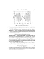
FEM computations
Based on the detailed knowledge of the geometry and the physical properties of different
materials,2DFEMfieldcomputations[3]are performedforsymmetrical andunsymmetrical
loads in magnetodynamics, on a small transfor mer of 3 kVA shown in Fig. 3.
Figure 3. Transformer of 3 kVA: Distribution of the magnetic field in the case of no-load.
III-3.5. Improved Modeling of Three-Phase Transformer Analysis 455
Load
Secondary windingsPrimary windings
V
V
V
Figure 4. Electrical circuit related to FEM computations.
The electric circuit related to different cases is shown in Fig. 4. One can notice the
primary, secondary windings, and the resistances of the load.
Measurements: Comparison of results
Case of no-load for a transformer Yy0 of 3 kVA, 380 V/232 V,
50 Hz, ucc = 3.26%

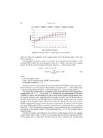
Fig.5showsthecomputed primary currents givenbythetwonumerical methods and relative
to a small transformer of 3 kVA in the case of no-load at rated voltage 380 V.
Figs. 6–8 show respectively the measured respectively computed primary currents i
A
,
i
B
, and i
C
relative to this case.
Table 1 shows results coming from different approaches in the case of no-load
for a transformer Yy0, without connecting the neutrals in the primary and secondary
sides.
Figure 5. Computed primary currents given by the two numerical methods in the case of no-load.
Figure 6. Computed and measured primary current i
A
in the case of no-load.
Figure 7. Computed and measured primary current i
B
in the case of no-load.
Figure 8. Computed and measured primary current i
C
in the case of no-load.
III-3.5. Improved Modeling of Three-Phase Transformer Analysis 457
Table 1. Comparison of results case of no-load for a transformer Yy0
Test results [A] Numerical approaches [A] FEM approaches [A]
I
A
0.803 0.745 0.75
I

B
0.52 0.515 0.531
I
C
0.76 0.744 0.749
Case of no-load for a transformer Dy5 of 3 kVA, U = 230 V
Figs. 9–11 show the measured respectively computed line primary currents relative to a
coupling Dy5 in the case of no-load, under a voltage of 1.045 p.u.
Figure 9. Computed and measured primary current i
1A
in the case of no-load.
Figure 10. Computed and measured primary current i
1B
in the case of no-load.
458 Kawkabani and Simond
Figure 11. Computed and measured primary current i
1C
in the case of no-load.
Table 2. Comparison of results case of symmetrical load for a
transformer Yy0
Test results [A] Numerical approaches [A] FEM approaches [A]
I
A
3.4 3.18 3.19
I
B
3.34 3.25 3.24
I
C
3.63 3.41 3.37

I
a
5.4 5.26 5.26
I
b
5.38 5.26 5.23
I
c
5.38 5.26 5.19
Case of a symmetrical load in the secondary, the primary supplied
at its nominal voltage 380 V, Yy0
Table 2 shows results coming from different approaches in the case of a symmetrical load
connected to the secondary of the transformer (R
a
= R
b
= R
c
= 25 ) under nominal
voltage U
N
= 380 V, without connecting neutrals.
Case of an unsymmetrical load in the secondary
Table 3 shows results coming from different approaches in the case of an unsymmetri-
cal load connected to the secondary of the transformer (R
a
= 40.5 ; R
b
= 14.6 ; R
c

=
39.15 ;63.95% of unsymmetry) under nominal voltage U
N
= 380V, with the neutral
connected only in the secondary side. A measured zero-sequence inductance is taken into
account in the secondary side L
0s
= 1.9 mH.
III-3.5. Improved Modeling of Three-Phase Transformer Analysis 459
Table 3. Comparison of results case of unsymmetrical load for a
transformer Yy0
Test results [A] Numerical approaches [A] FEM approaches [A]
I
A
2.62 2.50 2.55
I
B
4.46 4.33 4.30
I
C
3.41 3.2 3.15
I
a
3.2 3.2 3.22
I
b
9.17 8.89 8.82
I
c
3.42 3.45 3.39

A very good agreement between results coming from different approaches and for dif-
ferent cases can be noticed (relative error less than 8% between different approaches).
The present approach will be applied to a large transformer of distribution (1,000 kVA,
Dyn11, 18,300/420 V).
Conclusions
In the present paper, a new approach for the three-phase transformer analysis is described.
This one based on equivalent magnetic circuit-diagrams takes into account the nonlinear
B-H curve and zero-sequence flux. The B-H curve is represented by a Fourier series
expression, which gives a smooth B-H curve, and permits the analytical determination of
all the inductances and their derivatives vs. the currents. A ver y good agreement between
results coming from different approaches is obtained.
References
[1] L. Guanghao, Xu Xiao-Bang, Improvedmodelingofthenonlinear B-H curve and its application
in power cable analysis, IEEE Trans. Magn., Vol. 38, No. 4, pp. 1759–1763, 2002.
[2] J J. Simond, A. Sapin, B. Kawkabani, D. Schafer, M. Tu Xuan, B. Willy, “Optimized Design of
Variable-SpeedDrivesandElectricalNetworks”,7thEuropeanConference onPowerElectronics
and Applications EPE’97, Trondheim, Norway, September 1997.
[3] FLUX2D, version 7.60/6b, CEDRAT.
Appendix: Numerical approach with the currents as state variables
For example, the voltage equation relative to the primary A is given by:
u
A
= R
A
·i
A
+
dψ
A
dt

+
dψ
01
dt
= R
A
·i
A
+ (L
σ A
+ L
h1A
+ L
01
) ·
di
A
dt
+ (L
AB
+ L
01
) ·
d
dt
i
B
+ (L
AC
+ L

01
) ·
d
dt
i
C
+ L
Aa
·
d
dt
i
a
+ L
Ab
·
d
dt
i
b
+ L
Ac
·
d
dt
i
c
+
dψ
A

dt
{
Val 1
}
+
dψ
B
dt
{
Val 2
}
+
dψ
C
dt
{
Val 3
}
460 Kawkabani and Simond
with:
Val 1 =
dR
1T
dψ
A

i
A
·
∂ L

h1A
∂ R
1T
+i
a
·
∂ L
Aa
∂ R
1T
+i
B
·
∂ L
AB
∂ R
1T
+i
b
·
∂ L
Ab
∂ R
1T
+i
C
·
∂ L
AC
∂ R

1T
+i
c
·
∂ L
Ac
∂ R
1T

Val 2 =
dR
2T
dψ
B

i
A
·
∂ L
h1A
∂ R
2T
+i
a
·
∂ L
Aa
∂ R
2T
+i

B
·
∂ L
AB
∂ R
2T
+i
b
·
∂ L
Ab
∂ R
2T
+i
C
·
∂ L
AC
∂ R
2T
+i
c
·
∂ L
Ac
∂ R
2T

Val 3 =
dR

3T
dψ
C

i
A
·
∂ L
h1A
∂ R
3T
+i
a
·
∂ L
Aa
∂ R
3T
+i
B
·
∂ L
AB
∂ R
3T
+i
b
·
∂ L
Ab

∂ R
3T
+i
C
·
∂ L
AC
∂ R
3T
+i
c
·
∂ L
Ac
∂ R
3T

and
∂ L
h1A
∂ R
1T
=
−N
2
1
· (R
2T
+ R
3T

)
2
(R
1T
· R
2T
+ R
1T
· R
3T
+ R
2T
· R
3T
)
2
Similar expressions are established for all the partial derivatives of inductances vs. the
magnetic reluctances R
1T
, R
2T
,R
3T
of the cores.