Recent Developments of Electrical Drives - Part 4 ppt

I-2. OPTIMIZED CALCULATION OF
LOSSES IN LARGE HYDRO-GENERATORS
USING STATISTICAL METHODS
Georg Traxler-Samek, Alexander Schwery, Richard Zickermann
and Carlos Ramirez
ALSTOM (Switzerland) Ltd., Hydro Generator Technology Center, CH-5242 Birr, Switzerland
, ,
,
Abstract. A very important issue during the electrical design of hydro-generators is the reliability
of the loss calculation in the manufacturer’s design calculation program. The design engineer who
has to guarantee the losses must be able to estimate the risk of liquidated damages when defining the
guarantee values. This paper presents the optimization of the loss calculation in a design program for
salient pole synchronous machines. Statistical methods are used to calibrate the loss calculation with
measurements made during commissioning. Within this paper special importance is attached to the
optimization of the no-load electromagnetic losses.
Introduction
In hydro power plants, the mechanical power of the water turbine is converted into electrical
power mainly by three-phase synchronous generators with salient poles (see Fig. 1). These
machines are built with an active power up to 800 MW. To reach the best efficiency of the
turbine the speed of the generator is adapted to the hydraulic conditions resulting in typical
speed ranges of generators from 67 to 1,500 rpm. The corresponding number of poles of
the salient pole machine start from 2p = 4upto2p = 90 for a 50 Hz grid.
Inthe basicdesign phaseofahydro-generator thedesign engineeroptimizesthe electrical
design regarding the electromagnetic load, the temperature rises, the losses, and the manu-
facturing costs without exceeding tolerable mechanical stresses in the machine at runaway
speed. The main problem when calculating power losses in hydro-generators are deviations
between the calculated and measured losses. These deviations can have several reasons:
1. Inaccuracies in the used loss calculation model,
2. Manufacturing tolerances,
3. Measuring tolerances during commissioning tests.
Especially when guaranteeing the losses, the design engineer must be able to estimate the

risk of liquidated damages.
The analytical losscalculation isbased onmathematical andphysicalcalculationmodels.
Due to the complexity of synchronous machines, inaccuracies in the loss calculation model
S. Wiak, M. Dems, K. Kom
˛
eza (eds.), Recent Developments of Electrical Drives, 13–23.
C

2006 Springer.
14 Traxler-Samek et al.
Figure 1. Hydro-generator during installation of the rotor.
cannot beavoided. Furthermore materialproperties are only known witha limited precision.
Especially in refurbishment projects such information is generally missing. In this case the
design engineer is obliged to roughly estimate some important material parameters. The
recalculation of the existing machine using the described loss calculation method can help
to get an idea about the material properties.
Tolerances in the manufacturing process (as a worn out stator lamination punching tool
for example) lead to non-predictable deviations between calculation and measurements.
Finally measurements are affected by errors even though they are carried out according to
international standards [1].
The uncertainties and the only limited accessibility for analytical algorithms make sta-
tistical methods a valuable help in order to improve the precision of the computed values
and consequently be in-line with site measurements made during commissioning tests.
Method of loss calibration
To calibrate the analytical loss calculation using measurements, a series of reference ma-
chines and a series of test machines were defined. The reference machines are used to
calibrate the losses by means of statistical methods, the test machines are used to validate
the loss calibration results.
In the electrical design program the analytical loss calculation is subdivided into N
parts assembled in an N dimensional lossvector p

T
c
= (P
1
P
N
). The components of this
vector are the result of an analytical calculation algorithm. The loss vector is scaled with
the measured sum of the loss components p
m
to get the dimensionless expression
p =
1
p
m
· p
c
(1)
I-2. Losses in Large Hydro-generators 15
By defining the N-dimensional vector o
T
= (1 1) we generally get
p
T
c
· o = p
m
resp. p
T
· o = 1 (2)

due to deviations between the calculated and measured losses. The aim is to get a good
accordance between computation and measurement by defining a weighting factor kj for
each of the N loss components
k = (k
1
k
N
) (3)
such that p
T
· k ≈ 1. The difference between the calculated and the measured value d is
defined by
d = p
T
· k −1 (4)
The set of M reference machines is introduced with its scaled loss vectors p
1
p
M
.
These vectors are assembled in a loss matrix
P =
⎛
⎜
⎝
p
T
1
.
.

.
p
T
M
⎞
⎟
⎠
=
⎛
⎜
⎝
p
11
··· p
1N
.
.
.
.
.
.
.
.
.
p
M1
··· p
MN
⎞
⎟

⎠
(5)
The deviation vector d(k) for a given set of weighting factors k including the set of
reference machines is derived from equation (4)
d(k) = P · k − o (6)
An optimized set of weighting factors k can be found by minimization of the mean
quadratic deviation δ
δ =

1
M
d(k)
T
· d(k) (7)
This can be done with different optimization algorithms. In the following example the
optimized factors are found by means of numerical methods described in [2].
No-load electromagnetic losses
The no-load electrical losses are the so-called Iron Losses. They are measured during
commissioning when the machine is excited at the rated machine voltage. All the other
losses, which exist at no-load operation with rated voltage (mechanical losses: air friction,
fan losses, bearing friction, and rotor copper losses for the no-load excitation current) are
subtracted and therefore not included in the Iron Losses.
The calculations and models shown in this document are based on research work from
different sources (e.g. [3–13]). Some methods were used with the already existing calcula-
tion method. Other methods are new and mainly based on recent works.
Numerical simulations with the Finite-Element method [14–16] were used to confirm
the analytical computations. For the integration in the calculation tool these methods would
be too time consuming. The used electromagnetic no-load loss model contains N = 10
different partial losses:
16 Traxler-Samek et al.

1. Stator iron losses in teeth P
1
and yoke P
2
These losses are calculated with the well-known formula
P
1,2
= k
Fe
· M · c(B, f ) (8)
where f is the grid frequency, M is the mass of the stator teeth/yoke, and the function
c(B, f ) defines the specific iron losses of the stator core lamination material in dependency
of the magnetic flux density B and the frequency f . The factor k
Fe
is based on experience
and contains the influence of the air-gap field Fourier expansion harmonics.
2. Eddy current losses on the pole shoe surface due to tooth ripple pulsation P
3
These losses are calculated according to the two-dimensional analytical model described in
[3]. In the air-gap region, the Laplace equation and in the pole shoe region, the Helmholtz
equation are solved. As shown in Fig. 2(a) the tooth ripple pulsation of the magnetic flux
density is replaced by a linear current density field wave
K(x, t) = K
0
· exp j(ωt − kx) (9)
where k is the wave number and ω the angular frequency of the tooth ripple pulsation.
Saturation effects are taken into account with a surrogate relative permeability μ
r
obtained
a)

b)
2D
2D
Air-gap
Pole shoe
clamping plate
finger
stator
stator tooth
yoke
e
x
e
x
e
y
e
y
e
x
e
y
2D
ΔA = 0
ΔA = 0
K(x,t)
.
e
z
e

z
K(x,t)
.
ΔA − jwmkA = 0
ΔA − jwmkA = 0
Figure 2. Analytical loss calculation models for the calculation of P3, P8, and P9.
I-2. Losses in Large Hydro-generators 17
iteratively in dependence on the tangential magnetic flux density on the pole shoe surface
B(H) = μ
0
μ
r
H. The 3D-effect of laminated poles is considered with a loss reduction
coefficient [7].
3. Eddy current losses in the upper strands of the stator winding due to the radial
magnetic field in the stator slot P
4
The radial magneticfield in the stator slotis composed of the magneticfield entering the slot
computed with Conformal Mapping [12] and the additional magnetic field due to the tooth
relief in case of saturated stator teeth. The eddy current losses in the strands are calculated
with a simplified formula [13].
4. Circulating and eddy current losses in the Roebel bars due to the parasitic end
region magnetic field P
5
,P
6
The parasitic end region magnetic field is obtained by a two-dimensional end region Bound-
ary Element modelshown in Fig. 3.The obtained2D magnetic fielddistribution isconverted
into cylindrical 3D-coordinates with
B

3D
(r,α,z) = B
2D
(r, z) ·exp(jpα) ·
D
2r
· f
p

d
τ
p

(10)
where α is the tangential angle, D is the stator bore diameter, r the radial coordinate, and
p the number of pole pairs. The function f
p
takes into account the influence of adjacent
poles with their negative orientation, d is the distance of the field calculation point from
Pole
Clamping plate
radial
axial
e
r
e
z
Air-gap
mm
0 100

end
Figure 3. Simplified two-dimensional Boundary Element model of the end region.
18 Traxler-Samek et al.
the air-gap end and τ
p
the pole pitch length. The circulating P5 and eddy current losses
P6 are calculated by methods described in [13]. The Roebel bar is replaced by a network
which contains the resistances, self- and mutual inductances of the strands. The parasitic
end region magnetic field is introduced by means of voltage sources.
5. Eddy current losses in the clamping fingers P
7
The magnetic field in the clamping fingers is also calculated with the Boundary Element
model shown in Fig. 3. The obtained magnetic flux density is corrected to take into account
the effect of the stator slots. This is done with Conformal Mapping depending on the local
slot geometry. The losses are calculated with a local eddy current model shown in [13].
6. Eddy current losses in the stator core end laminations P
8
The Boundary Elementmodel shown inFig. 3is used tocompute themagnetic field entering
the stator core end tooth laminations. The magnetic flux density is corrected to take into
account the effect of the stator slots (see item 5). The eddy current losses are computed by
means of a local eddy current model shown in Fig. 2(b), where the core end laminations
(solving the Helmholtz equation) and the surrounding air (Laplace equation) are modeled.
The lamination effect cannot be taken into account. The pulsating magnetic field on the end
laminations is introduced with a pulsating linear current density function
K(x, t) =
K
0
2
· (exp j(ωt − kx) +exp j(ωt + kx)) (11)
(angular frequency ω and wave number k), local saturation effects are taken into account

iteratively (see item 3).
7. Eddy current losses in the stator clamping plates P
9
The calculation of the eddy current losses in the stator clamping plates is also based on
the Boundary Element model (Fig. 3). The obtained magnetic flux density field wave on
the clamping plates is applied to a local calculation model displayed in Fig. 2(b) [13]. The
calculation method is similar to the calculation of eddy current losses in the stator core end
laminations (item 6), the exciting magnetic field wave is introduced with a surrogate linear
current density field wave
K(x, t) = K
0
· exp j(ωt − kx) (12)
(angular frequency ω and wave number k), local saturation effects are again considered by
iteration (see item 3).
8. Losses in the damper bars due to tooth ripple pulsations in the air-gap
magnetic field P
10
For the calculation of losses in the damper bars a simplified asynchronous squirrel cage
model is applied. Neitherthe effect of the d- andq-axes nor the effect of a damper displace-
ment are taken into account.
I-2. Losses in Large Hydro-generators 19
Speed/rpm
800
600
400
200
0
0 100 200 300 400
Rated output
/MVA

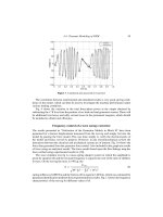
Figure 4. Range of reference and test machines used for the loss calibration tests.
Recalculation of existing machines
It is necessary to have a good and possibly large set of reference and sample machines. For
all of these machines, anew electrical recalculation is performed using not only the original
electrical calculation, but also a set of drawings with detailed information regarding
r
The main dimensions: This is necessary, to be sure to get the electrical calculation of the
machine which was actually built.
r
Material parameters: It is obvious, that an exact knowledge of the used materials (for
example the stator core lamination quality) is necessary.
r
Additional dimensions: For the new loss calculation, some parameters, which were not
taken into account in the old calculation must be available.
r
Measurements: The measurement of the no-load test with rated voltage excitation and if
possible also the air-gap measurement (stator roundness) must be available.
The loss evaluation method presented above is used to calibrate the no-load losses of
largesynchronous machines withsalient poles. Asshown in Fig. 4, aset of various machines
is taken into account.
Optimization of theno-load electromagnetic losses
The aim of the statistical evaluation as described above is to find an optimum set of loss
calibration weighting factors k = (k
1
k
N
) where N = 1, ,10. The range of these
factors can be limited in order to allow the optimization process to take only physically
meaningful factors into consideration:
k

min
≤ k ≤ k
max
(13)
The limits are set very carefully taking into account experience, certain detailed mea-
surements and the results of special investigations.
20 Traxler-Samek et al.
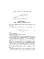
Importance / %
60
40
20
0
P
1
P
2
P
3
P
4
P
5
P
6
P
7
P
8
P
9

P
10
Figure 5. Importance of different loss types. Average, minimum, and maximum values.
To compare the optimum set of weighting factors with the classical calculation method
the weighting factor k
old
is defined, where the factors for the new developed partial losses
are set to zero. Furthermore a not-calibrated set of weighting factors k
0
is defined where all
factors are set to one.
The relative importance of the partial losses P
1
, ,P
10
is shown in Fig. 5. The stator
core losses in teeth P
1
and yoke P
2
are the most important items followed by eddy current
losses in the clamping plates P
9
and eddy current losses in the pole shoe surface due to
tooth ripple pulsation P
3
. The high variation shows, that the order of importance can change
significantly depending on the machine type.
The final evaluations are made with different sets of reference and test machines: Two
runs were made with fixed evaluation factors (k

old
and k
0
) and different evaluation runs
were made with different distributed groups of M = 21 reference- and 12 test machines.
The loss calibration weighting factors were evaluated by minimizing the mean quadratic
deviation.
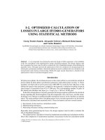
The deviation histogram showing the frequency distribution of deviations d for the old
calculation method using the weighting factor k
old
is shown in Fig. 6, whereas the deviation
histograms for the new calculation method are displayed in Figs. 7 and 8. Fig. 7 shows the
frequency distribution with all evaluation weighting factors set to one, Fig. 8 shows the best
evaluation run.
In all deviation histograms, a negative deviation means a more pessimistic calculation
(higher losses calculated than measured) and consequently a positive deviation a too op-
timistic calculation (lower losses calculated than measured). The vertical lines show the
±20% and ±10% deviation band. The hatched bars (left bars) in Fig. 8 represent the test
machines taken into account to test the loss calibration results while the white bars (right
bars) represent the reference machines taken into account for the evaluation.
The new calculation method shows significant better results than the old calculation
method. Even in the not-calibrated run, where all weighting factors are set to one, the
frequency distribution of the deviations shows a smaller standard deviation. The loss
I-2. Losses in Large Hydro-generators 21
Deviation / %
−50
0
2
4
6

8
10
N
umber of machines
Lower losses
calculated than
measured
Higher losses
calculated than
measured
−30 −10 0 10 30 50
Old Method
Figure 6. Frequency distribution of deviations d between calculation and measurement for the old
loss calculation method.
Deviation / %
−50
0
2
4
6
8
1
0
Number of machines
Higher losses
calculated than
measured
−30 −10 010 30 50
New Method - Not Calibrated
Deviation / %

−50
0
2
4
6
8
10
Number of machines
Lower losses
calculated than
measured
Higher losses
calculated than
measured
−30 −10 0 10 30 50
New Method - Not Calibrated
Figure 7. Frequency distribution of deviations d between calculation and measurement for the new
loss calculation method, all evaluation factors set to one.
calibration with the best set of weighting factors does not improve the standard deviation
but centers the deviations (mean value close to zero).
Conclusion
The presented calculation method shows that the loss calculation can be improved signif-
icantly with the help of statistical methods. The standard deviation of the frequency plot
allows for an estimation of the risk when defining the guaranteed losses during a tender. As
it is very time consuming to collect all the necessary machine data, the given calculation
example uses only 33 reference- and test machines. For a good statistical statement this is
22 Traxler-Samek et al.
Deviation / %
−50
0

2
4
6
8
10
Number of machines
Lower losses
calculated than
measured
Higher losses
calculated than
measured
−30 −10 0 10 30 50
New Method - Best Run
Figure 8. Frequency distribution of deviations d between calculation and measurement for the new
loss calculation method after the loss calibration using a set of 21 reference- (white bars) and 12 test
machines (hatched bars).
not enough. As the calibration process is an ongoing work it will be improved in the future
with more and more measured machines.
The new method provides much more detailed results allowing the electrical design
engineer to have a good idea of critical parts in the machine like the pole end design, the
stator core end design and the winding overhang. This simplifies the decision process for
special and cost-intensive design improvements like stepping or slitting of the stator core
end laminations.
References
[1] IEC 60034-2, Rotating Electrical Machines. Part 2: Methods for Determining Losses and Effi-
ciency of Rotating Electrical Machinery from Tests (excluding machines for traction vehicles),
International Electrotechnical Commission, Switzerland, 1972.
[2] T. Coleman, M.A. Branch,A. Grace, Optimization Toolbox, For Use with MATLAB
R


: User’s
Guide, The Math Works, Inc., United States, 1990–1999.
[3] M.G. Barello, Courants de Foucault engendr´es dans les pi`eces polaires massives des alterna-
teurs par les champs tournants parasites de la r´eaction d’induit. Rev. Gen. Electr., Vol. 64,
Issue 11, pp. 557–576, 1955.
[4] H. Bondi, K.C. Mukherji, An analysis of tooth-ripple phenomena in smooth laminated pole-
shoes, Proc. IEE, Vol. 104 C, pp. 349–356, 1957.
[5] F. Fiorillo, A. Novikov, An improved approach to power losses in magnetic laminations under
nonsinusoidal induction waveform. IEEE Trans. Magn., Vol. 26, No. 5, pp. 2904–2910, 1990.
[6] J. Greig, K. Sathirakul, Pole-face losses in alternators, Proc. IEE, Vol. 108 C, pp. 130–138,
1961.
[7] J.Greig,E.M.Freeman,Simplifiedpresentationoftheeddy-current-loss equation for laminated
pole-shoes, Proc. IEE, Vol. 110, pp. 1255–1259, 1963.
[8] St.Kunckel,G.Klaus,M. Liese, “CalculationofEddyCurrentLosses and TemperatureRisesat
the Stator End Portion of HydroGenerators”,Proceedings on the 15thInternational Conference
on Electrical Machines, ICEM, Brugge, Belgium, August, 2002.