Recent Developments of Electrical Drives - Part 10 ppsx

76 Rembowski and Pelikant
Figure 3. Generated meshes for the shit larger than one third of the air gap width.
Taking into account the stator node with number j neighboring with nodes i and i + 1
of the rotor mesh, f the linear interpolation the equation for this node can be described as
follows (5):
V
J
θ
i
− V
i
(γ
i
) − V
i+1
(θ
i
− γ
i
) = 0 (5)
Where θ
i
is the angle between nodes with the numbers i and i +1, and γ
i
is the angle
between the stator mesh node j and the rotor mesh node i.
j+n+1
i+k+2
j+n
j
i

i+k
j+n-i
i+k-1
j+n-2
j-1
j-2
i-1
i-2
i+2
i+1
Figure 4. Part of the one level(z =const.) of the mesh with the overlappingregion(parts of electrodes
dashed, dimensions enlarge)—symmetrical air gap.
I-7. Analysis of Electrostatic Microactuators 77
j+n+1
i+k+2
j+n
j
i
i+k
j+n-i
i+k-1
j+n-2
j-1
j-2
i-1
i-2
i+2
i+1
Figure 5. Part of the one level(z =const.) of the mesh with the overlappingregion(parts of electrodes
dashed, dimensions enlarge)—nonsymmetrical air gap.

In the nonsymmetrical model nodes of the stator and the rotor meshes for overlapping
bounds have different angle θ and radius r (Fig. 5). The stator mesh node with number j
neighbors with four nodes i, i + 1, i +k, and i + k + 1 of the rotor mesh.
The equation describing the value of the potential in the j node can be written down
using bilinear interpolation function in the following form (6):
V
j
(γ
i
, r
i
) = a
0
γ
i
r
i
+ a
1
γ
i
+ a
2
r
i
+ a
3
(6)
Using equation (6) for each node at both boundaries (outer for the rotor mesh and inner
for the stator mesh) one obtains sub matrix of main matrix [M] containing five nonzero

elements for each row. As a result one gets nonsymmetrical system of linear equations,
which is solved using LDU decomposition method with permutation matrix (7).
[M] = [P][L][D][U][
˜
P] (7)
Presented algorithm was implemented in a numerical program, which allows determining
a field distribution for every angular position of the rotor and every possible movement of
its rotation axis.
Integral parameters
The application allows calculating integral parameters for every position of the rotor—in
particular the system energy that can be written down in general in form (8):
W =


wd =




E
0
D dE

d (8)
78 Rembowski and Pelikant
According to Maxwell stress tensor, formula defining force components can be described
as follows (9):
F =

S

1
ε

(D × n)D −
1
2
|
D
|
2
n

dS =

ε

S
E
2
n
− E
2
t
2
dS

n +

ε


S
E
n
E
t
dS

t
(9)
Using explicit choose shape functions λ
i
in formula (8), one can calculate the total system
co-energy as the sum of the energy accumulated in each of the mesh elements (10).
W =

e


e

ε


e
grad
2
V
i
λ
i

d
e

(10)
Proceeding in the same way with the general expression (9) leads to formulas describing
force components in relation to surface S, which consists of the sum of elementary surfaces
S
i
in the single mesh elements. As the result one obtains the normal force component in
form (11):
F
n
=
ε
0
2

i

S
i
(grad
2
n
V
i
λ
i
− grad
2

t
V
i
λ
i
) dS
i
(11)
By analogy the tangent force components can be written down as follows (12):
F
t
=

i

S
i

ε
0
(grad
n
V
i
λ
i
· grad
t
V
i

λ
i
)

dS
i
(12)
Numerical verification
The basis of the verification of the presented model was the numerical experiment. Air gap
energy was calculated in the part common for both the rotor and the stator meshes and
obtained results were compared. The quality of energy calculation was determined on the
basis of numerical testing of the convergence of the solutions from both meshes (Figs. 6
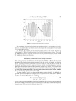
and 8). Theinfluence of mesh density on the value of energy accumulated inthe air gap was
analyzed for different positions of rotor (rotation and shift). It allows determining minimal
mesh density for given accuracy of computations. A clear tendency of both curves to reach
the same value was observed. It means a convergence of energy value and exact value.
The convergence was observed ir respective of the rotor’s location. However, the slope of
the curve changes, which results from different energy values for different locations of the
rotor.
At the same time the difference between the energy value calculated from stator mesh
and the energy value calculated from rotor mesh was computed (Fig. 7). Convergence to
zero of the above difference was observed. Like before the tendency appears irrespective
of the rotor’s position.
Convergence of solutions determined on the basis of the values of potentials in the
nodes of both rotor and stator meshes confirm the thesis that the implemented model is
correct.
I-7. Analysis of Electrostatic Microactuators 79
Figure 6. Influence of the mesh density on the value of air gap energy for rotor position 0
◦
.

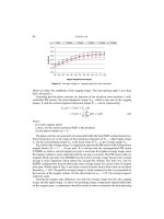
Calculating the changes of energy value for different rotor angular position (Fig. 9)
allows determining static torque as follows (13).
M =
∂W
∂γ
(13)
As a matter of fact, the approach based on Maxwell’s tensor is used (11, 12), whereas the
above formula (13) is only a method of confirming the correctness of the results.
Figure 7. Influence of the mesh density on the value of air gap energy for rotor position 30
◦
.
80 Rembowski and Pelikant
Figure 8. Ratio of air gap energy calculated from stator and rotor meshes.
Figure 9. Dependence of air gap energy on the rotation angle of the rotor (about 25,000 mesh
elements).
Conclusions
Another step in developing the model will be extending it to the analysis of microacutators
with leant rotation axis. It will require interpolation by three variable function and not one
variable function (symmetrical model)or twovariable function (model withshifted rotation
axis) as so far.
I-7. Analysis of Electrostatic Microactuators 81
The most important conclusion resulting from the carried out studies on the three-
dimensional model forthe analysis of theelectrostatic micromotors isthat it allowseffective
analysis for any position of the rotor—both rotation and rotation axis shift.
Presented algorithm allows correct and exact representation of the changing width air
gap in the model. Since significant part of the main matrix rows is calculated only once and
it’s only recalculated fragment is the one representing the air gap, it is possible to reduce
computation time.
The results of the numerical tests confirm the thesis about the correctness of the model.
Short computation times are obtained even with quite big number of mesh elements.

References
[1] G. Hainsworth, D. Rogger, P. Leonard, 3D finite element modeling of conduction supports in
coilguns, IEEE Trans. Magn., Vol. 31, No. 3, pp. 2052–2055, 1995.
[2] M. Mehergany, S.F. Bart, L.S. Tavrow, J.H.Lang, S.D.Senturia, M.F. Schelecht, A studyofthree
microfabricated variable capacitance motors, Sens. Actuators, A21–A23, pp. 173–179, 1990.
[3] A.Pelikant,Analizapolowo-obwodowasilnik´owelektrostatycznychielektromagnetycznychza-
silanychimpulsowo,WydawnictwoPolitcchnikiL
 odikicy, ZesrytyNauKowenr 908, Rozprowy
Naukowe, Z. 111 2002.
[4] R. Perrin-Bit, J. Coulomb,A three dimensionalfine elements meshconnection for problem with
movement, IEEE Trans. Magn., Vol. 31, No. 3, pp. 1920–1923, 1995.
[5] I. Tsukerman, Overlapping finite elements for problems with movement, IEEE Trans. Magn.,
Vol. 28, No. 5, pp. 2247–2249, 1992.
I-8. COUPLED FEM AND SYSTEM
SIMULATOR IN THE SIMULATION OF
ASYNCHRONOUS MACHINE DRIVE
WITH DIRECT TORQUE CONTROL
S. Kanerva
1
, C. Stulz
2
, B. Gerhard
3
, H. Burzanowska
2
,J.J¨arvinen
3
and S. Seman
1
1

Laboratory of Electromechanics, Helsinki University of Technology, P.O. Box 3000, FI-02015
HUT, Finland
sami.kanerva@hut.fi, slavomir.seman@hut.fi
2
ABB Switzerland Ltd, Large Drives, Austrasse, CH-5300 Turgi, Switzerland
,
3
ABB Oy, Electrical Machines, P.O. Box 186, FI-00381 Helsinki, Finland
, jukka.jarvinen@fi.abb.com
Abstract. A compound drive simulator is presented, where a finite element method (FEM) model
of the electric motor is coupled with a frequency converter model and a closed-loop control system.
The method is implemented for SIMULINK and applied on a 2-MW asynchronous machine drive.
The results are validated by measurements and the performance is compared with an analytical motor
model. It is shown that simulation with the FEM model provides very good results and gives much
better insight in the motor behavior than the analytical model.
Introduction
As the demands for performance of electric drive systems increase, also the simulation
software must follow the requirements. Designers of frequency converters and electric
motors rarely work in the same location, but they must be able to model both parts of the
drive as accurately as possible. Naturally, different expertise is required to model electrical
machines or power electronics, but the key issue is to couple these models together in a way
that experts in both fields can profit from each other by using the most advanced simulation
models in their design.
Accurate modeling of digital control systems requires simulation in multiple timescales,
because different sampling times are used for measurement, filtering, estimation, and mod-
ulation. By including all detailed functions and sample times, it is possible to create very
accurate simulation modelsof the converter control. In such a case, however, also a detailed
electrical machine model is needed in order to get the maximum advantage of the drive
model.
Finite element method (FEM) is a widely known method to model electrical machines

with high accuracy. For standard-type machines, two-dimensional field solution coupled
S. Wiak, M. Dems, K. Kom
˛
eza (eds.), Recent Developments of Electrical Drives, 83–92.
C

2006 Springer.
84 Kanerva et al.
with simple circuit equations of the windings is usually accurate enough, when the cross-
section geometry and material properties are known [1].
The most problematic in the drive simulation is to couple the FEM computation with the
converter model. Most obvious method would be to couple the converter model in the FEM
code and solve all the equations simultaneously with uniform time steps [2,3]. However,
such an approachis hardly applicable to a detailed converter model with digitalclosed-loop
control because of the amount of programming, and the demand for common time step
length would make the simulation too heavy with respect to existing computing facilities.
Reference [4] presents an indirect method for coupling time-stepping FEM simulation
with SIMULINK using multiple sample times for different parts of the system model. The
method was applied to a cage induction motor and a frequency converter with direct torque
control (DTC). The model of the control system was developed in order to investigate
control-related topics and verified for steady-state and transient operation of the drive. In
its original state, it was using a motor model that was based on analytical equations.
In this paper, thesame method isapplied to an asynchronous motor drive withDTC. The
frequency converter modelis based ona realapplication, comprising adetailed model of the
digital control system. The frequency converter model is implemented in SIMULINK and
it is coupled with a two-dimensional FEM model of the asynchronous motor. The system
is simulated in steady-state and transient operation, and the simulation results are validated
by a comparison with the measured results.
Compound model of inverter-fed electrical drive
The general structure of the compound drive simulator is shown in Fig. 1. The model

is implemented in SIMULINK but the execution of the model is controlled from within
Script file:
runA6ka.m
Input data
- Environment
- Model
- Operating
- Starting
conditions
Calculation of
initial conditions
Setup of
SIMULINK
Run simulation
Output results
(Plots, )
Parameters Management Speed ControlTorque Control
Motor
Inverter
Plot files
DC circuit
3-Phase
3-Level
Inverter
Motor
Process
Measurements
Inverter control
Model
Overall

DC voltage
Phase
voltages
Torque Speed
Phase
currents
Half DC
voltages
DC currents
Speed reference
Torque
reference
Flux reference
Inverter control
Measurements
Flux reference
Speed
control
Torque reference
Load
model
Speed reference
conditions
Figure 1. General structure of the drive simulator.
I-8. Coupled FEM and System Simulator 85
+
–
neutral
to motor
Overall DC

voltage
Figure 2. Simulation model of the three-phase three-level inverter.
MATLAB. This allows to specify the plant parameters, operating and starting conditions
very easily. Based on the selected operating conditions, theinitial conditions for continuous
and discrete time states are determined. This allows to start the simulation in a reasonably
stable operating point. The machine model in this drive simulator can be selected to be the
simple analytical or the precise FEM-based model.
The main components of the simulated plant are DC circuit, inverter, motor, process,
and control. Two basic control schemes can be selected: torque or speed control.
Inverter and DC link
The three-level inverter is modeled as a set of ideal switches, which can connect the phase
voltages to either plus, neutral, or minus potential of the DC links. Fig. 2 gives a rough
overview. The switching pattern is given by the drive control. The status of the switches
together with the phase currents determines the currents in the DC bus bars of the DC link.
The current in the neutral bus bar is used to calculate the potential of the neutral point of
the DC link. The phase voltages transferred to the motor terminals are defined by DC link
voltages and switching pattern.
Analytical motor model and load
The analytical motor model is used for simulations that will be compared to the FEM-based
motor model.It isbased onthe well-known space vector representationof theasynchronous
machine. Ituses boththe stator and the rotor fluxes as statevariables. The followingfeatures
are present in the model:
r
constant air-gap and sinusoidal flux distribution along the air-gap
r
no iron losses
r
resistances and inductances are independent of frequency and temperature
r
the magnetizing inductance can saturate with increasing main flux

Themodel needs phase voltagesandspeedasinputsandproduces phase currents and air-gap
torque as outputs.
The driven process is described by the differential equation of motion. A single inertia is
used. The loadtorque mayfollow several functions of the speed (constant, linear, quadratic,
or mixed). The mechanical mass is driven by the electromagnetic torque of the motor and
gives the speed as output.
86 Kanerva et al.
v3_vs
v3_s
A6ka
VECTOR v3_s
Vector -> Switching
me
t_load
n
Mechanical
System
n_rot t_load
Load Model
Inverter
Induction
Machine
Model
(analytical
or FEM)
Current
Meas.
Speed
Meas.
v3_s

v3_is
vdc1_t2
vdc2_t2
n_rot
VECTOR
Control_dtc6000_AD
vdc_id
Voltage
Meas.
Figure 3. Model of the drive system implemented in SIMULINK.
Control
The control model describes speed/torque control using a DTC algorithm. The main func-
tions ofthe ACS6000drive areimplemented asdiscrete functions on different time levels to
appropriately represent the behavior of the real drive. The detailed description of the DTC
control cannot be in the scope of this paper.
The top level of the SIMULINK environment is shown in Fig. 3.
Model of the asynchronous motor
Modeling by finite element method (FEM)
The FEMmodel ofthe motor is based ontwo-dimensional finiteelement method and circuit
equations of the windings [1]. The magnetic field in the core region is calculated using
magnetic vector potential formulation, in which the vector potential and current density
have only z-axis components.
The phase windings in the stator or rotor are modeled as filamentary conductors with
uniformly distributed current flowing through all the coils that belong to the same phase.
The rotor bars aremodeled assolid conductors,inwhichthecurrentdensity variesaccording
to eddy currents. The sources of the magnetic field are the phase currents, the voltage drop
in the rotor bars and the magnetic force of the permanent magnets, depending on the type
and construction of the machine.
The relations between voltage and current are determined in the circuit equations of
the stator and rotor windings, which also include the end-winding impedances and the

short-circuit rings. As a result, only phase voltages are needed as an electrical input for
the FEM model. The electromagnetic torque is calculated by virtual work principle, and the
movement of the rotor is determined from the equation of motion. At each time step, new
position is calculated for the rotor and the air-gap mesh is refined.
FEM block for SIMULINK
The FEM computation is implemented as a functional block in SIMULINK using dy-
namically linked program code (S-function), as illustrated in Fig. 4. The stator voltage