Recent Developments of Electrical Drives - Part 17 ppsx

II-1. High-Frequency Position Estimators 151
By using (36), the high-frequency current vector, observed from the estimated system (

qd ),
is given by
i
dq
s,i
(θ
r
,

θ
r
,ω
i
t) =

I
0
+ I
1
· e
j2(θ
r
−
ˆ
θ
r
)


cos(ω
i
t) (42)
By removing the offset I
0
in (40) or in the modulus of the current in (42) and by using
the inverse tangent function, the argument of the exponential function in (40) or in (42)
is calculated. From this result, the rotor angle can be estimated. It follows from I
1
in (39)
that the higher the value of L, the higher the resolution of a position estimation, which is
already concluded for an estimator that uses PWM generated pulses.
Estimation errors
As mentioned before, in most position estimators the magnetizing current direction is
approximated by the d-axis direction. However, for high loads, the controller forces an
important stator current along the q-axis. This means that the magnetizing current direction
deviates from the d-axis. Consequently, the model in (22) or (24) introduces an estimation
error. Compensating this error is done in [5,6] by measuring the error during the self-
commissioningofthe drive.Theerror can alsobepredictedbysimulatingthe drive,modeled
with (10), with an estimator that uses a high-frequency voltage pulse train and that is based
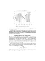
on (22). The simulation results as a function of μ are presented in Fig. 5. The error on
θ
r
is zero if the magnetizing current is aligned with one of the magnetic axes. The higher
the deviation of i
m
from the d-axis, the higher the estimation error; an increased error
is shown if saturation becomes more important. However, as permanent demagnetization
of the magnets has to be avoided and the stator current has to be limited, the results are
meaningful for small deviations of μ from π/2 only.

Figure 5. Estimation error on the rotor angle of an IPMSM as a function of μ for various magnetic
states in the case of an approximated magnetizing current.
152 De Belie et al.
Figure 6. Estimation error onthe rotor angle of anIPMSM as a function ofβ in the case ofneglecting
the presence of multiple saliencies.
In most estimators the influence of multiple saliencies on the current response is consid-
ered as a source of disturbance. Simulating an unloaded IPMSM, with (10) and (18), and a
position estimator, that uses a PWM generated high-frequency voltage and equation (22),
predicts the estimation error. Simulation results, based on a multiple saliency as modeled
in Fig. 4, are shown in Fig. 6. Clearly, the error on θ
r
oscillates as a function of β.
Conclusions
This paper discusses fundamental equations used in high-frequency signal based IPMSM
position estimators. For this purpose, a small signal dynamic flux model is presented that
takesintoaccountthenonlinearmagneticcondition and themagneticinteractionbetween the
direct and thequadrature magnetic axis. An addition to the model is proposedto tackle mul-
tiple saliencies. Using the novel equations some recently proposed motion-state estimators
are described. It is shown that the higher the inductance difference between the two orthog-
onal magnetic axes, the higher the position estimation resolution. Furthermore simulation
results reveal the estimation error caused by estimators that neglect the presence of multiple
saliencies or that approximate the magnetizing current angle by π/2.
References
[1] M. Schr¨odl, Sensorless controlof permanent magnetsynchronous motors, Electr. Mach. Power
Syst., Vol. 22, No. 2, pp. 173–185, 1994.
[2] E. Robeischl, M. Schr¨odl, Optimized INFORM measurement sequence for sensorless PM
synchronous motor drives with respect to minimum current distortion, IEEETrans. Ind. Appl.,
Vol. 40, No. 2, pp. 591–598, 2004.
[3] M.J. Corley, R.D. Lorenz, Rotor position and velocity estimation for a salient-pole permanent
magnet synchronous machine at standstill and high speeds, IEEE Trans. Ind. Appl., Vol. 34,

No. 4, pp. 784–789, 1998.
[4] M. Linke, R. Kennel, J. Holtz, “Sensorless PositionControl of Permanent Magnet Synchronous
Machines Without Limitation at Zero Speed”, Proceedings of the 28th Annual Conference of
the IEEE Industrial Electronics Society, Sevilla, Spain, CD-ROM, November 5–8, 2002.
[5] C. Silva, G.M. Asher, M. Sumner, K.J. Bradley, Sensorless rotor position control in a surface
mounted PM machine using HF rotating injection, EPE J., Vol. 13, No. 3, pp. 12–18, 2003.
[6] M. Schr¨odl, “Zuverl¨assigkeit sensorloser INFORM-geregelter Permanentmagnetmotor-
Antriebe im Transient-betrieb bis Stillstand”, Elektrotechnik und Informationtechnik, Heft 2,
pp. 48–57, Febuary 2004.
[7] U.H. Rieder, M. Schr¨odl, “Optimization of Saliency Effects of External Rotor Permanent
Magnet Synchronous Motors with Respect to Enhanced INFORM-Capability for Sensorless
Control”, Proc. of the 10th European Conference on Power Electronics and Applications,
Toulouse, France, CD-ROM, September 2003.
II-1. High-Frequency Position Estimators 153
[8] M.W. Degner, R.D. Lorenz, Using multiple saliencies for the estimation of flux, position, and
velocity in AC machines, IEEE Trans. Ind. Appl., Vol. 34, No. 5, pp. 1097–1104, 1998.
[9] J.A.A. Melkebeek, “Small Signal Dynamic Modelling of Saturated Synchronous Machines”,
Conf. Proc. Int. Conf. El. Mach., Lausanne, Switzerland, Part 2, September 18–21, 1984,
pp. 447–450.
[10] J.A.A. Melkebeek, J.L. Willems, Reciprocity relations for the mutual inductances between
orthogonal axis windings in saturated salient-pole machines, IEEE Trans. Ind. Appl., Vol. 26,
No. 1, pp. 107–114, 1990.
II-2. SENSORLESS CONTROL OF
SYNCHRONOUS RELUCTANCE MOTOR
USING MODIFIED FLUX LINKAGE
OBSERVER WITH AN ESTIMATION
ERROR CORRECT FUNCTION
Tsuyoshi Hanamoto, Ahmad Ghaderi, Teppei Fukuzawa
and Teruo Tsuji
Kyushu Institute of Technology, 2-4 Hibikino, Wakamatsu-ku, Kitakyushu 808-0196, Japan

, ,
Abstract. The modified flux observer with an estimation error correct function for the sensorless
control method of synchronous reluctance motor is presented. The validity of the proposed method
is verified by experiments. The experimental setup is based on the Real Time Linux for operating
system and Field programmable Logic Array interface board.
Introduction
Recently, a motor control for a motion control is widely used in various industrial applica-
tions. AC motors are better to be used because they have some advantages, such as easiness
of maintenance. In addition, sensorless speed control of the AC motors has been proposed
for the demand of the reduction of weight, size, and total cost.
Synchronousreluctancemotor(Syn.RM)is akindoftheACmotorsandhastheadvantage
that it is mechanically simple and robust because they need not the permanent magnet for
a material of a rotor, then many researchers are proposed the sensorless algorithm [1–4].
In this paper, we propose a novel sensorless control method for Syn.RM. The sensorless
control is based on the modified flux linkage observer, which is proposed by authors for
permanent magnet synchronous motors (PMSM) [5]. The observer is able to estimate the
modified flux linkage and the electromotive force (EMF) simultaneously, and the motor
speed and the rotor position are calculated from these estimated values. But as same as the
other method, the precision of the observer-based estimation is affected by the parameter
fluctuations [7]. In this paper, we propose the new estimation method for Syn.RM using the
modified flux linkage observer with an estimation error correct function. A Proportional-
Integral (PI) type controller is added to the system to compensate the estimation error. It
operates that the estimated magnitude of the flux corresponds to the nominal value.
The high-speedexperimental systemis required to achieve the proposed methodbecause
the observer matrix is changed for every control period and the gains must be recalculated.
S. Wiak, M. Dems, K. Kom
˛
eza (eds.), Recent Developments of Electrical Drives, 155–164.
C


2006 Springer.
156 Hanamoto et al.
Thus, the experimental setup is based on the Real Time Linux (RTLinux) [8] for operating
system. The RTLinux is used for achievement of the real time control and it guarantees
to satisfy hard real time constraints in light of maintaining soft real time requirements. To
acquire the data from sensors and to output the gate signals to the system, the interface
board is accomplished designed by the Field programmable Logic Array (FPGA).
The environment of the system development is so convenient and sophisticated to com-
bine the RTLinux operating system and the FPGA-based interface board.
The validity of the proposed method is verified by experiments.
Mathematical model of Syn.RM
Fig. 1 shows the mathematical model of Syn.RM, where d, q show the dq axes rotating at
ω
e
,α,β show αβ axes, u, v, w show three phase axes, θ
e
shows the electrical angle from α
(or u) axis and ω
e
= dθ
e
/dt.
The voltage equations of the Syn.RM in αβ axes are described as follows

v
α
v
β

=


R + PL
α
0
0 R + PL
α

i
α
i
β

+ PL
β

cos 2q
e
sin 2q
e
sin 2q
e
−cos 2q
e

i
α
i
β

(1)

where, v: armature voltage, i:armature current, R: armature resistance, L: armature induc-
tance, P: differential operation (= d/dt), subscript
d,q denotes d-axis component, q-axis
component, respectively.
L
d
, L
q
are calculated using, L
α
, L
β
as follows

L
d
L
q

=

11
1 −1

L
α
L
β

(2)

q axis
n axis
b axis
a axis
u axis
d axis
w axis
w
e
w
e
q
e
Figure 1. Analytical model of synchronous reluctance motor.
II-2. Sensorless Control of Syn.RM Using Modified Flux Linkage Observer 157
Equation (1) is rewritten as follows [2] when the de-coupling controlfor dq axes is achieved
in the speed control system of the Syn.RM

v
α
v
β

= R

i
α
i
β


+ P

y
α
y
β

(3)
where, flux linkage y
α
, y
β
are defined as follows,

y
α
y
β

=

L
α
+ L
β
cos 2q
e
L
β
sin 2q

e
L
β
sin 2q
e
L
α
− L
β
cos 2q
e

i
α
i
β

(4)
Use the well-known relationship described in (5), y
α
, y
β
are calculated as follows,
cos 2q
e
= 2 cos
2
q
e
− 1 = 1 −2 sin

2
q
e
sin 2q
e
= 2 sin q
e
cos q
e




(5)

y
α
y
β

= L
q

i
α
i
β

+ (L
d

− L
q
)

cos q
e
0
0 sin q
e

cos q
e
sin q
e
cos q
e
sin q
e

i
α
i
β

(6)
When we set
Y = (L
d
− L
q

)i
d
, (7)
the flux linkage are described as follows.

y
α
y
β

= L
q

i
α
i
β

+ Y

cos q
e
sin q
e

(8)
Y is able to be treated as a constant because it changes slowly compared with the sampling
period. Then the derivative of (8) is
P


y
α
y
β

=

PL
q
i
α
−Yw
e
sin q
e
PL
q
i
β
Yw
e
cos q
e

(9)
In this paper, the EMF of each axis (e
a
, e
b
) are determined as the following equation.

e
α
=−Yw
e
sin q
e
e
β
= Yw
e
cos q
e




(10)
Finally, (3) is described as follows.
P

i
α
i
β

=
⎡
⎢
⎢
⎣

R
L
q
0
0 −
R
L
q
⎤
⎥
⎥
⎦

i
α
i
β

−
1
L
q

e
α
e
β

+
1

L
q

v
α
v
β

(11)
This equation is equivalent of the equation for a PMSM [5], then we can also apply the flux
linkage observer for the Syn.RM.
Sensorless speed control method of Syn.RM
Modified linkage observer with an estimation error correct function
In this chapter, we consider the estimation method of the rotor speed and the position.
The EMF is assumed that it consists the fundamental component, which rotate the con-
stant angular speed, w
e
and the DC component denoted as follows. The DC component is
158 Hanamoto et al.
not necessary in theideal case, but in the real systemthis term is very effective for the ripple
reduction of the estimated speed calculation.

e
α
e
β

=

A

α
cos q
e
+ B
α
sin q
e
+ e
α0
A
β
cos q
e
+ B
β
sin q
e
+ e
β0

=

e
α1
+ e
α0
e
β1
+ e
β0


(12)
From (8), the following equation are obtained.

y
α
y
β

=

y
α
− L
q
i
α
y
β
− L
q
i
β

=

Y cosq
e
Y sinq
e


(13)
The derivative of the EMF is given by the following equation.
P

e
α
e
β

=

−w
2
e
Y cosq
e
−w
2
e
Y sinq
e

=−w
2
e

y
α
y

β

(14)
But in the practical case, the estimated rotor position has the estimation error, and L
d
,
L
q
are considered as a function of an armature current. So, we propose to use the following
equation instead of (14), where K
y
is a compensation coefficient.
P

e
α
e
β

=−K
y
w
2
e

y
α
y
β


(15)
Finally, the voltage equation of α-axis is written as
Px = Ax + bv
α
, (16)
where,
x =

i
α
y
α
e
α1
e
α0

T
A =
⎡
⎢
⎢
⎢
⎢
⎣
R
L
q
0 −
1

L
q
−
1
L
q
0010
0 −K
y
w
2
e
00
0000
⎤
⎥
⎥
⎥
⎥
⎦
(17)
b =

1
L
q
000

T
To apply the same manner for β-axis, the flux linkage and the EMF of β phase are also

obtained.
How to calculate the coefficient K
y
is as follows.
1. The magnitude of the flux linkage is estimated by
Y =

y
2
α
+ y
2
β
(18)
2. K
y
is obtained the output of the PI controller shown in Fig. 2. In the figure, the flux
linkage reference Y
n
is calculated by the nominal values of the inductance and the d-axis
reference i
∗
d
.
Y
n
= (L
d
− L
q

)i
∗
d
(19)
3. For every control period, K
Y
in (17) is recalculated.
4. K
Y
is convergence to the appropriate value after several iterations.
II-2. Sensorless Control of Syn.RM Using Modified Flux Linkage Observer 159
Figure 2. Estimation error correct function.
The flux linkage and theEMF are estimateddirectly applying the full order observer to (16).
The speed reference ω
∗
and the voltage reference v
∗
α
are used instead of ω
e
and v
α
because
these values are not measured in this system.
To convert the discrete time system at control period T
s
, the following equation is
obtained.
x(k + 1) = (A
d

− g
d
c
d
) x(k) + b
d
v
∗
α
(k) + g
d
i
α
(k) (20)
where,
A
d
= e
−AT
s
b
d
=

T
s
0
e
Aτ
dτ ·b

g
d
= (
g
1
g
2
g
3
g
4
)
c
d
= (
1000
)
g
d
is the observer gain in the discrete time system. We select the observer gains to have all
of the poles of (A
d
− g
d
c
d
) on the real axis in unit circle as the multiple poles.
In the proposed method, A
d
is changed because K

Y
is calculated for every control period
and it is also the function of the speed reference. Though the online calculation is required
to convert the discrete time system and calculation of the observer gains, the computer
technology able to achieve the calculation within 200 μs.
Speed and position estimation
The estimated speed w
e
are obtained by the following equation. A low pass filter (LPF) is
added after the output of w
e
in the experimental system.
w
e
=
e
β1
y

α
− e
α1
y

β
y

2
α
+ y


2
β
(21)
Since it is enough to estimated the sin q
e
and cos q
e
instead of the rotor position (q
e
)
itself, then
sin q
e
=
y
β

y
2
α
+ y
2
α
, cos q
e
y
α

y

2
α
+ y
2
α
(22)
160 Hanamoto et al.
Experimental results
Experimental setup
To realize the validity of the control theory, there is a need for an appropriate operating
system that could operate in real time. The PC-based control offers great advantages like
a faster design cycle and increased productivity [6]. Here, we refer to the real time system
based on the RTLinux [8].
The RTLinux is a hard real time operating system that handles time-critical tasks and
runs the normal Linux as its lowest priority execution thread. Then the system includes the
networking, GUI programming, and several other function.
We can construct the PC-based experimental setup which includes not only the control
program but also the user GUI, for example, data entry windows of the reference, controller
gains, and so on. Fig. 3 is an example of the GUI using RTiC-Lab [9], which is a semi-
detached open source software designed to run on the RTLinux.
From the viewpoint of the hardware, the digital servomotor control system requires
a speed detector, a position detector, both for reference, the PWM pulse generator, and
the interface circuit. In this paper, we designed the interface circuit board, which in-
cludes all of the necessary functions. Fig. 4 shows the interface board that consists
of the Field programmable Logic Array (FPGA), 10 MHz system clock, and an A/D
converter.
An Altera FLEX10K50 is selected for the FPGA device and the circuit is designed
using the VHDL, which is one of the hardware description languages. The speed and
Figure 3. GUI controller using RTiC.
II-2. Sensorless Control of Syn.RM Using Modified Flux Linkage Observer 161

Figure 4. Interface board using the FPGA.
position detectors with speed correction function, clock generator for A/D converter, and
ISA interface circuit are designed in it.
Fig. 5 shows the configurationof the experimental system consists of the RTLinux-based
PC, an inverter, an interface board using the CPLD device, and the tested motor. Table 1
shows the specification of the tested motor.
Experimental results
Figs. 6 and 7 show the ramp response where the speed command is changed from 500 to
1,500/min. Fig. 6 shows the results when the sensor is used for the speed control. Here, the
dashed line shows the estimated speed and the solid line shows the speed calculated by the
Figure 5. Configuration of the system.