Recent Developments of Electrical Drives - Part 23 pot

212 Schlensok and Henneberger
Table 1. Cases for different force excitations
Type of excitation Rotational direction
Stator-teeth Left-hand
Rotor-teeth Right-hand
Stator-teeth Right-hand
Rotor- and stator-teeth Right-hand
values are positioned on the side of the mounting-plate. Left-hand rotation results in max-
imal excitation locations on the opposite side of the machine. For this, both directions are
computed and the audible acoustic-noise radiation is compared.Fig. 1 defines the rotational
direction.
Usually it is sufficient to simply take the force excitation of the stator in to consideration
to make good predictions of theradiated noise. The stator ofthe regarded machineis weakly
coupled to the casing mechanically spoken by hard rubber rings around the casing caps and
steel-spring pins in the notches of the stator and casing. The rotor on the other hand is
strongly coupled to the casing caps by the bearings. For this, the rotor excitation has to be
taken into account as well for comparison reasons.
Electromagnetic simulation
The first step of the computational process is the electromagnetic simulation. The induction
machine is simulated with a three-dimensional magnetostatic model, which uses stator and
rotor currentsasexcitations.Dueto computational timesaving reasonstherotor-bar currents
are derived from a two-dimensional, transient computation [5]. The 2D model consists of
6,882 first order triangular elements and the computation of one time step in 2D takes
rubber ring
feed
through
z
screw hole
mounting notches
mounting plate
left–hand

rotation
Figure 1. Definition of rotational direction; location of the mounting plate, the mounting notches,
the screw holes, and the rubber rings.
II-7. Comparison of Stator- and Rotor-Force Excitation 213
t
2D
= 24.7 s. A 3D time-step simulation takes t
3D
= 494 min due to 288,782 first order
tetrahedral elements in the 3D model. The duration of the transient phenomenon t
tp
equals
the rotor-time constant t
r
:
t
tp
= t
r
≈ 0.1 s (1)
Depending on the time step t (t
3D
= 416.6 μs) the number of time steps “lost” N
lost
for
analysis is:
N
lost
=
t

tp
t
= 240 (2)
In the case of transient 3D simulation the extra simulation time would approximately sum
up to:
t
extra
= N
lost
· t
3D
− N
lost
· t
2D
= 3, 576h = 149d (3)
The 3D static simulation can be performed simultaneously on several computers. So that
the effective computational time is reduced drastically to about 3 weeks in total, for both:
the 2D transient and 3D static simulation.
Two global results are provided:
1. the net force onto the rotor and
2. the torque of the machine for each time step.
Due to the symmetry of the machine only a half model has to be applied and the radial
and tangential components of the net force cannot be computed. Therefore, only the axial
component of the net force and the torque are analyzed. All electromagnetic simulations
are performed employing the open-source software iMOOSE of the IEM [6].
The studied point of operation is at nominal speed n
N
= 1,200 rpm and f
1

= 48.96 Hz.
N = 120 time steps are computed and analyzed with the 3D model. For the 2D model the
equivalent time steps are taken into regard.
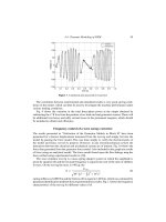
The time behavior of the axial component of the net force, which depends only on the
skewing angle is depicted in Fig. 2. The average value is F
z
= 9.22 N. The direction of
the force depends on the rotational direction. In the case of left-hand rotation the force acts
0
–3
–6
–9
–12
–15
–18
0.0
0.01 0.02
0.03 0.04
0.05
t [s]
F
z
[N]
F
z 3D–static
Figure 2. Net-force behavior for 3D model.
214 Schlensok and Henneberger
0.0
0.01 0.02
0.03 0.04

0.05
t [s]
T [Nm]
T
3D-static
T
2D-transient
4.5
4.2
3.9
Figure 3. Torque behavior for 2D and 3D model.
in negative z-direction (see Fig. 1). For right-hand rotation the rotor is dragged into the
opposite direction.
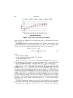
Fig. 3 shows the time behavior of the torque for 2D transient and 3D static computation.
The average value of the 3D torque is lower because of the rotor skewing and the front
leakage: M
3D
= 4.13 Nm < 4.31 Nm = M
2D
. Both effects are neglected by the 2D model.
The net-force and the torque behavior are analyzed using the Fast-Fourier Transformation
(FFT) [7]. Due to the smaller time step in the case of the two-dimensional simulation t
2D
= 1/3t
3D
the cut-off frequency f
co,2D
in the spectrum is three times f
co,3D
= 1,200 Hz.

The time step t
3D
and the number of time steps N
3D
in case of the 3D simulation are
chosen in such a way that the resolution in the frequency domain is exactly the rotor speed
f
R
=20 Hz. The resolution of the 2D spectrum is 10 times that of the 3D spectrum because
of the high number of time steps N
2D
= 3,600. With the Criteria of Nyquist [8] and
 f =
2 · f
co
N
(4)
the resolutions of the spectra result in:
 f
3D
= 20 Hz and  f
2D
= 2 Hz (5)
Fig. 4 shows the spectrum of the axial net-force component of the 3D simulation.
The main orders found are at intervals of f
int
= 240 Hz. The same orders are found
in the torque spectrum in Fig. 5. This reflects the very close link of the axial net-force
component and the torque: The torque vector points into the axial direction. Structure-
borne sound-measurements show the highest values at 720 and 940 Hz next to others.

These two significant orders might be caused by the axial force and torque excitation. The
spectrum of the 2D simulation is similar to Fig. 5.
Next to these two global values the electromagnetic computation also provides the flux-
density distribution for each time step. From this the surface-force density is derived at the
interface of air and the lamination of the machine [9].
Only the 3D model is regarded for the investigations in the following. For each time step
the surface-force density of the stator and rotor lamination are computed of the 3D model.
II-7. Comparison of Stator- and Rotor-Force Excitation 215
f [Hz]
F
z
[N]
F
z,3D
(f)
0
220
480 720 960
10
5
2
1
5
2
10
–1
Figure 4. Spectrum of the axial net-force component of the 3D model.
The excitation of each considered element is analyzed by using the FFT and transforming
the forces to the frequency domain.
The surface-force density-excitation for one time step is depicted in Fig. 6. The highest

values are reached at the up-running edges of the stator teeth.
The surface-force excitation is transformed to the frequency domain as well. The FFT
is again used. In a first step the values of the three components (x, y, and z) of all N =
120 time steps of each stator-surface element are collected. There are E
stator
=20,602 shell
elements. Then the FFT is performed for each of these elements. Finally the transformed
values for the three components are rearranged into two files (real and imaginary part) for
each of the frequencies in the spectrum (number of frequencies: N
f
= 61).
Structural-dynamic simulation
The next step in the computational process is the simulation of the deformation of the entire
machine str ucture due to the surface-force density-excitation derived from the electromag-
netic simulation. For this, an extra model of the entire machine is generated consisting of
the stator and rotor laminations including the winding and the squirrel cage, the shaft, the
bearings, the casing, and the casing caps. The model is described more detailed in [1].
f [Hz]
T [Nm]
T
3D
(f)
0
220
480
720
960
5
2
1

5
2
5
5
2
10
–2
10
–1
Figure 5. Spectrum of the torque of the 3D model.
216 Schlensok and Henneberger
Figure 6. Surface-force density-excitation for one time step at left-hand rotation.
Four different types of force excitations are object of investigation as listed in the intro-
duction section of this paper. The locations of the highest force excitations depend on the
rotational direction. In the case of right-hand rotation the maximal forces arise at the side
of the mounting-plate of the machine (see Figs. 1 and 6). For left-hand rotation the highest
excitation is located on the opposite side.
Exemplarily, Fig. 7 shows the real and the imaginary part of the surface-force density-
excitation for f = 420 Hz for left-hand rotation. There is a phase shift between both parts.
This will result in a pulsating deformation behavior for the excitation at this frequency. The
maximal forces in both, the real and imaginary part, are positioned at four locations. The
order of deformation does not depend on the rotational direction.
The frequenciesanalyzed and the resulting mechanical orders of deformationr are listed
in Table 2. r =2 is themost often orderfound.Mainly secondandfourth orderdeformations
are detected. Orders higher than r = 6 usually do not produce strong deformation and are
not critical in respect of noise radiation. The most important order is the elliptical second
order [10].
The resulting deformation of the stator and the casing of the machine in the case of
pure stator-teeth excitation is shown in Fig. 8 in an overemphasized representation for the
frequency of f = 620 Hz.

The spring pins keeping the statorfixed inthe casing dampthe deformationand decouple
both parts very well. The deformation of the casing is much lower than that of the stator
and cannot be sensed in the figure. Some deformation orders are shown in Fig. 9.
Fig. 10 depicts the real part of the deformation of the entire machine structure in scalar
representation at f =720 Hz. Although the order of deformation of the stator deformation
is r
stator
= 2 the deformation order of the casing of the machine is r
casing
= 4. This effect
stems from the skewing and the mounting of the machine. The skewing results in torsional
vibrations [5]. The machine is mounted on one front plate. This way the deformation is
II-7. Comparison of Stator- and Rotor-Force Excitation 217
Table 2. Mechanical orders
of deformation found for all
analyzed frequencies
rf(Hz)
2 420, 520, 720, 940
4 100, 1,040, 1,140
6 620
Figure 7. Location of the maximal surface-force density-excitation for f = 420 Hz at left-hand
rotation: (a) real part. (b) Imaginary part.
218 Schlensok and Henneberger
Figure 8. Deformation of the stator at f = 620 Hz.
Figure 9. Mechanical orders of the deformation.
(a) r = 2. (b) r = 4. (c) r = 6.
Figure 10. Deformation of the entire machine in the case of pure stator-teeth excitation, real part.
II-7. Comparison of Stator- and Rotor-Force Excitation 219
(a) Stator-Teeth Excitation,
Left-Hand Rotation,

f = 720 Hz.
(b) Stator-Teeth Excitation,
Right-Hand Rotation,
f = 720 Hz.
Figure 11. Deformation of the entire machine structure: pure rotor, pure stator, and combined rotor-
stator excitation.
“reflected” at this stiff front plate and produces the double order on the opposite front plate
(“open end”). Inthecaseof right-hand rotation themaximaldeformation arisesonthe “open
end” of the structure. This is the same location of the maximal force excitation. Therefore,
the deformation of the machine depends strongly on the rotational direction.
In a nextstep the deformationstemmingfromthecombinedrotor- and stator-excitationat
right-hand motion is simulated. Exemplarily Fig. 11 depicts the real part of the deformation
for pure rotor excitation (Fig. 11(a)), pure stator-excitation (Fig. 11(c)), and for combined
excitation (Fig. 11(c)) at f = 940 Hz. All three pictures show the same scaling (black
strong, white weak deformation).
Pure rotor excitation results in strong deformation of the shaft and the casing caps. This
deformation mainly deforms these parts in radial and axial direction of the machine. If
pure stator-excitation is regarded mainly the casing at the “open end” and the outer parts of
the casing caps are deformed. Finally the combination of both excitations results in strong
deformation of the casing and the casing caps. These observations are stated for all studied
frequencies listed in Table 2.
Next to the possibility of using the deformation of the structure for acoustic simulation
the structure-borne sound at certain locations can be derived. For this reason the node
nearest to the location of the accelerometer for measurements on the flank of the casing and
one node on the casing cap where the converter is mounted are chosen. Fig. 12 shows the
locations of the nodes regarded with their IDs. The definition of the tangential, radial, and
axial direction is displayed as well.
The structure-borne sound-level L
S
is calculated as follows for radial, tangential, and

axial direction:
L
S
= 20 · log
a
1 μm/s
2
dB (6)
a is the acceleration of the specific node at the regarded frequency f [1].
Fig. 13 depictsthe str ucture-bornesound-levels for someselected frequencies inthe case
of left-hand rotation and pure stator-teeth force-excitation. The axial sound-level is about
L
S
=20 dB lower throughout the spectrum. This fact can be stated for right-hand rotation
220 Schlensok and Henneberger
Figure 12. Locations of the nodes for structure-borne sound-analysis.
and both pure stator and combined rotor- and stator-excitation as well. The same levels are
reached for the tangential and radial components for all regarded frequencies.
Referring to the deformation plot in Fig. 11(a) Fig. 14 shows exemplarily the results for
the levels calculated on thecasing cap(Node 3041)in thecase ofpure rotor-force excitation
for Node 3041. The three components reach nearly the same levels. The highest values are
detected for f = 620 Hz and f = 720 Hz.
Fig. 15 depicts the levels in the case of pure stator-excitation (see Fig. 11(c)) for Node
3041. Except for much lower levels at f = 100 Hz and f = 620 Hz slightly lower values
are reached for f = 720 Hz. The axial component is the lowest for f = 620 Hz and the
higher frequencies similar to the results in Fig. 13.
Finally the combined stator- and rotor-excitation is regarded (Fig. 16). At Node 3041 the
spectrum is similar to pure stator-excitation with the exception of the significantly higher
levels at f = 620 Hz and f = 720 Hz. This spectrum suits the result of the acceleration
measurements very well.

It can be stated that pure stator-excitation results in fairly good estimations con-
cerning the structure-borne sound-levels. Only very few orders are affected significantly
Figure 13. Structure-borne sound-levels, left-hand rotation, pure stator excitation, ID 5457.
II-7. Comparison of Stator- and Rotor-Force Excitation 221
Figure 14. Structure-borne sound-levels, right-hand rotation, pure rotor excitation, ID 3041.
Figure 15. Structure-borne sound-levels, right-hand rotation, pure stator excitation, ID 3041.
Figure 16. Structure-borne sound-levels, right-hand rotation, combined stator-rotor excitation, ID
3041.