Recent Developments of Electrical Drives - Part 26 pps

II-9. Diagnosis of Induction Machines 243
2β
r
flux
sensor
ls
L
Ls
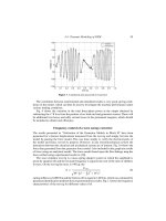
Figure 2. Measured flux.
If thesensor hasn turns and it has a rectangular shape of S area, and considering that l 
r, then the 
h,k
flux components regarding to the external flux density ones, are expressed
by:

h,k
(r)
= nS
sin(hpβ)
hpβ
ˆ
bn
a
h,k
(r)
cos kωt (31)
Then,toobtainthecomponentatthekω angular frequency,it is necessarytoaddthedifferent
terms which have this same frequency.

k
(r)

=
+∞

h=−∞

h,k
(r)
(32)
The terms which compose 
k
(r)
are very numerous but many do not contribute significantly.
Actually,relation(30)showsthatonlythetermswithasmallvalueofh willhaveaprominent
effect. This property is enhanced by the quantity
sin(hpβ)
hpβ
which appears in expression (31).
The data given by the coil is a voltage which results of the Lenz law. Consequently,
the e
k
(r)
components of the corresponding measured e.m.f. are obtained by the following
relation:
e
k
(r)
=−
d
k
(r)

dt
e
k
(r)
=−kωnS
+∞

h=−∞
sin(hpβ)
hpβ
K
h
(r)
ˆ
b
g
h,k

sin kωt (33)
It can be noticed that the electro-motive force spectra amplify the high frequencies, what
permits to distinguish the slot spectral lines more easily.
244 Thailly et al.
Figure 3. Experimental device.
Principle of measurements
The synoptic of the Fig. 3 shows the experimental device that allows performing the mea-
surement of the radial magnetic field component. The principle is to pick up the sensor
signal with an analyzer via an acquisition card.
A small winded flux sensor, with nS = 30 × 10
−3
, has been realized. It is located at a

distance r equals to 100 × 10
−3
m.
The tests are made consideringa star connected4 poles, 4kW,380/660 V, 50 Hz squirrel-
cage induction machine with 36 stator slots and 44 rotor bars. For this machine, Rs
int
=
60 × 10
−3
m, Rs
ext
= 90 × 10
−3
m.
The stator is supplied by 380 r.m.s. phase to phase voltage. The supply current is equal to
I =1.5 A. In order to neglectthemagneticeffects generated bytherotor,theslipiscloseto0.
Results
In the measured spectrum of the e.m.f. only the spectral lines corresponding to kr = 0
(fundamental) and kr =±1 will be considered for the comparison with the theory.
Concerning the fundamental, it is measured 5 × 10
−3
V (r.m.s. value). As the machine
is underfed, it will be supposed that the maximum of the flux density in the air-gap is 0.6 T.
In that case, assuming that the flux density component at 50 Hz is mainly composed of one
p pair pole wave (h = 1,
ˆ
b
g
1,1
= 0.5 T), μ

r
have to be equal to 600. This low value can be
justified taking into account that the frame is of cast iron and that the relative permeability
of this material is about 300.
For the harmonics, Table 1 gives the relative magnitudes of the frequencies of the couple
at [1 ± N
r
(1 − s)] f regarding to their fundamental.
Table 1. Relative magnitudes of the frequencies of the couple at [1 ± N
r
(1 −s)] f
regarding to the fundamental
[1 − N
r
(1 − s)] f [1 + N
r
(1 − s)] f
Calculation without K
h
correction coefficient −5.49 db −5.93 db
Calculation with K
h
correction coefficient −31.72 db −22.31 db
Calculation with K
h
and with prominent
components
−31 db −22.7bd
Practical spectral lines −27.06 db −18.84 db
II-9. Diagnosis of Induction Machines 245

–60
1000 1050
[1 – N
r
(1-s)]f [1 + N
r
(1-s)]f
1100 1150 1200
Practical values
Theoretical values
with K
n
correction coefficient
Theoretical values
without K
n
correction coefficient
f(Hz)
–40
–20
0
db
Figure 4. Comparison between practical and theoretical toothing spectral lines in relative values
regarding to the fundamental.
The two first table lines correspond to computation results where kr and ks vary from
−5to5andhs varies from 1 to 13.
The third table line gives the computation results where only the prominent components
depending on their number of pole pairs are considered.
For the spectral line at [1 − N
r

(1 − s)] f frequency (kr =−1), the lowest number of
pole pairs is obtained for hs = 1 and ks = 1; in that case, equation (8) gives |h|p = 2.
For this at [1 − N
r
(1 − s)] f frequency (kr =+1), ks =−1 and hs =−5 leads to con-
sider a prominent component such |h|p = 6.
The latest table line gives the relative magnitudes of this couple of frequencies which
are obtained by experimentation.
The results show that considering only the prominent component which composes one
spectral line is sufficient in the study of the external magnetic field.
Fig. 4 gives a graphic illustration of the results. It can be observed that when only the
analyticalexpressionofthe electro-motiveforceis computed,withouttake the K
h
correction
coefficient into account, the frequencies of the couple at [1 ± N
r
(1 − s)] f have similar
magnitudes which are high toward the magnitude of the fundamental.
When the K
h
coefficient is introduced to modify the magnitudes of the components
which compose the spectral lines, it can be noticed, in one hand, that the frequencies of this
same couple do not have yet the same magnitudes, and on the other hand, that the difference
with practical results is reduced (the error is only about 4 dB).
Let us also precise that the b
g
expression given by (7) shows that current harmonics are
induced in the stator windings and the rotor bars. These currents have been neglected in our
246 Thailly et al.
study but some of them contribute to define the magnitude of the considered spectral lines.

That can partially justify the deviations.
Conclusion
It is shown that all the flux density components do not evolve, through the stator, in the
same way according to the pole pair number hp of this component. So, it is determined the
correction to apply on the calculated air-gap flux density components in order to appraise
the measured spectrum outside of the machine.
The presented method permits to analyze a practical spectrum toward a reference one
obtained by calculation, that is specific for each machine.
Thisquantitativeapproachisinterestingiffaults are introduced in the modeling of the air-
gap flux density. In fact, the effects of the faults in the external magnetic field, considering
the pole number of the flux density components which are generated, can be precisely
predetermined.
Acknowledgment
This work is part of the project “Futurelec 2” within the “Centre National de Recherche
Technologique (CNRT) of Lille.”
References
[1] W.T. Thomson, M. Fenger, Current signature analysis to detect induction motor faults, IEEE
Ind. Appl. Soc. Meet. (IAS Magazine), Vol. 7, No. 4, pp. 26–34, 2001.
[2] M.E.H. Benbouzid, Bibliography on induction motors faults detection and diagnosis, IEEE
Trans. Energy Convers., Vol. 14, No. 4, pp. 1065–1074, 1999.
[3] H. H´enao, T. Assaf, G.A. Capolino, “Detection of Voltage Source Dissymmetry in an Induction
MotorUsingthe MeasurementofAxial LeakageFlux”,Proceedings ofInternationalConference
of Electrical Machines (ICEM 2000), Espoo Finland, August 2000, pp. 1110–1114.
[4] D. Belkhayat, R. Romary, M. El Adnani, R. Corton, J.F. Brudny, Fault diagnosis in induction
motors usingradial field measurement with an antenna, Inst. Phys. Meas. Sci. Technol., Vol.14,
No. 9, pp. 1695–1700, 2003.
[5] D. Roger, O. Ninet, S. Duchesne, Wide frequency range characterization of rotating machine
stator-core laminations, Eur. Phys. J. Appl. Phys., pp. 103–109, 2003.
[6] J.F. Brudny, Etude quantitative des Harmoniques du Couple du Moteur asynchrone triphas´e
d’Induction, Th`ese d’Habilitation, No. H29, Lille, France, 1991.

[7] J.F. Brudny, Mod´elisation de la Denture des Machines asynchrones. Ph´enom`ene de resonance,
J. Phys. III, pp. 1009–1023, 1997.
[8] K.J. Bins, P.J. Lawrenson, Analysis and Computation of Electric and Magnetic Field Problems,
Oxford: Pergamon press, 1973.
[9] Ph.L. Alger, The Nature of Induction Machines, 2nd edition, New York: Gordon & Breach
Publishers, 1970.
II-10. IMPACT OF MAGNETIC
SATURATION ON THE INPUT-OUTPUT
LINEARIZING TRACKING CONTROL OF
AN INDUCTION MOTOR
D. Dolinar
1
, P. Ljuˇsev
2
and G.
ˇ
Stumberger
1
1
Faculty of Electrical Engineering and Computer Science, University of Maribor,
Smetanova 17, SI-2000 Maribor, Slovenia

2
Ørsted DTU Automation, Technical University of Denmark, Elektrovej, Building 325, DTU,
DK-2800 Kgs. Lyngby, Denmark

Abstract. This paper deals with the tracking control design of an induction motor, based on input-
output linearization with magnetic saturation included. Magnetic saturation is accounted for by the
nonlinear magnetizing curve of the iron core and is used in the control design, the observer of state
variables, and in the load torque estimator. Experimental results show that the proposed input-output

linearizing trackingcontrolwith the included saturationbehaves betterthantheone without saturation.
It also introduces smaller position and speed errors, and better motor stiffness.
Introduction
The magnetic saturation phenomenon, which occurs in the induction motor (IM) iron core,
has been recognized from the very beginning of IM use. The models of saturated induction
machines presented in the literature [1–3] show that magnetic saturation is most frequently
considered by nonlinear variable mutual inductance, while the additional magnetic cross-
couplings are neglected. In general, leakage flux path saturation is rarely included in the
models, although its role in the squirrel-cage IM with closed rotor slots can be rather high.
The level of idealization, introduced by neglecting magnetic cross-saturation, depends on
the type of model, i.e. on the selected state variables [4].
Although magnetic saturation of the IM is very important for the performances of the
controlled drive, it has hardly ever been properly considered in control design because of its
mathematical complexity. Pioneering efforts to address the perturbing effects of magnetic
saturation on the field oriented control are found in [5].
Saturated induction motor models found in the literature [1,3] are used primarily for the
analysis of an induction machine operation. Some exceptions in which linear cascade rotor
S. Wiak, M. Dems, K. Kom
˛
eza (eds.), Recent Developments of Electrical Drives, 247–260.
C

2006 Springer.
248 Dolinar et al.
field oriented control is used can be found in [6–8] but they present an incomplete solution
for the control algorithm. An observer for state variables that includes magnetic saturation
is found in [9]. Some nonlinear control approaches, based on modified IM models that
include saturation, are given in [10–13] as well.
In this paper an input-output linearizing tracking control design is presented. It is based
on the mixed “stator current vector i

s
, rotor flux linkage vector Ψ
r
” saturated IM model
introduced by [3]. The effect of magnetic cross-saturation is totally included in the main
flux path saturation. The saturation of the stator and rotor leakage flux path is neglected. In
addition, a state variable observer and a load torque estimator were designed with included
magnetic saturation.
An i
s
, Ψ
r
saturated IM model is presented in this paper. The input-output linearization
based on the introduced modelis carried out,with respect to the rotorposition. Toobtain the
required unmeasurable state variables, an observer based on the inverse saturated IM model
was designed. The experimental results of the proposed input-output linearizing tracking
control of IM with included magnetic saturation show better dynamic performances of the
drive than the classical control, where magnetic saturation is not considered. The main
improvements are the smaller rotor position and speed errors, as well as higher stiffness
and better load torque rejection, which results in a smaller stator current when the motor is
loaded with a step change in the load torque [14].
Saturated induction machine model
The general approach to IM modeling incorporating magnetic saturation with different
selections of state variables is presented in [3]. The standard two-phase model of an IM in
the general reference frame with stator current vector i
s
and rotor flux linkage vector Ψ
r
as
state variables, is given by a nonlinear model (1)

u = A(x)
dx
dt
+ B(x)x
J
dω
r
dt
=
(
t
e
− t
l
)
− f ω
r
(1)
where
u =

u
sd
u
sq
00

T
x =


i
sd
i
sq
ψ
rd
ψ
rq

T
A(x) =
⎡
⎢
⎢
⎢
⎢
⎢
⎢
⎢
⎢
⎣
L
l
−
L
2
rl
L
dd
−

L
2
rl
L
dq
1 −
L
rl
L
dd
−
L
rl
L
dq
−
L
2
rl
L
dq
L
l
−
L
2
rl
L
qq
−

L
rl
L
dq
1 −
L
rl
L
qq
0010
0001
⎤
⎥
⎥
⎥
⎥
⎥
⎥
⎥
⎥
⎦
II-10. Impact of Magnetic Saturation of Induction Motor 249
B(x) =
⎡
⎢
⎢
⎢
⎢
⎢
⎢

⎢
⎢
⎢
⎢
⎢
⎢
⎢
⎣
R
s
−ω
g

L
l
−
L
2
rl
L
r

0 −ω
g
L
m
L
r
ω
g


L
l
−
L
2
rl
L
r

R
s
ω
g
L
m
L
r
0
−R
r
L
m
L
r
0
R
r
L
r

−ω
sl
0 −R
r
L
m
L
r
ω
sl
R
r
L
r
⎤
⎥
⎥
⎥
⎥
⎥
⎥
⎥
⎥
⎥
⎥
⎥
⎥
⎥
⎦
t

e
= p
L
m
L
r
(i
sq
ψ
rd
−i
sd
ψ
rq
)
u
sd
, u
sq
and i
sd
, i
sq
are the d- and q-axis stator voltages and currents, ψ
rd
and ψ
rq
are the
rotor flux linkages, R
s

and R
r
are the stator and rotor resistances, L
m
is the mutual static
inductance, L
s
and L
sl
are the stator self-inductance and the stator leakage inductance,
L
r
and L
rl
are the rotor self-inductance and the rotor leakage inductances, L
l
= L
sl
+ L
rl
is the total leakage inductance, L
dq
is the cross-coupling inductance, L
dd
and L
qq
are the
inductances along d- and q-axis, ω
g
is the angular speed of the general reference frame,

ω
r
is the rotor angular speed, ω
sl
= ω
g
− ω
r
is the slip angular frequency, J is the drive
moment of inertia, f is the coefficient of viscous friction, t
e
and t
l
are the electrical and the
load torque, and p is the number of pole pairs. Inductances L
dd
, L
qq
, and L
dq
are given as
follows:
1
L
dd
=
1
L
rl
+ L

cos
2
ρ
m
+
1
L
rl
+ L
m
sin
2
ρ
m
1
L
qq
=
1
L
rl
+ L
m
cos
2
ρ
m
+
1
L

rl
+ L
sin
2
ρ
m
,
m
=
|
Ψ
m
|
1
L
dq
=

1
L
rl
+ L
−
1
L
rl
+ L
m

cos ρ

m
sin ρ
m
, i
m
=
|
i
m
|
(2)
L
m
=

m
i
m
, L =
d
m
di
m
, cos ρ
m
=
ψ
md

m

, sin ρ
m
=
ψ
mq

m
where i
m
is the modulus of the magnetizing current vector. L represents the so-called
dynamic inductance, ψ
md
and ψ
mq
are the d- and q-components of the magnetizing flux
linkage vector Ψ
m
, ρ
m
is the angle of magnetizing flux linkage vector Ψ
m
, while 
m
is the
modulus of Ψ
m
. L
m
and L are given by equations (2) and are obtained from the measured
magnetizing curve presented in Fig. C1, Appendix C.

Two-phase i
s
, Ψ
r
model (1) can be written in the state-space form as:
dx
dt
=−A(x)
−1
B(x)x + A(x)
−1
u = Cx +ω
g
Zx + ω
r
Wx + Du
(3)
dω
r
dt
=
p
J
L
m
L
r
(i
sq
ψ

rd
−i
sd
ψ
rq
) −
1
J
t
l
−
f
J
ω
r
250 Dolinar et al.
where:
C =
⎡
⎢
⎢
⎣
c
11
c
12
c
13
c
14

c
21
c
22
c
23
c
24
c
31
0 c
33
0
0 c
42
0 c
44
⎤
⎥
⎥
⎦
Z =
⎡
⎢
⎢
⎣
z
11
z
12

z
13
z
14
z
21
z
22
z
23
z
24
000z
34
00z
43
0
⎤
⎥
⎥
⎦
W =
⎡
⎢
⎢
⎣
00w
13
w
14

00w
23
w
24
00 0 w
34
00w
43
0
⎤
⎥
⎥
⎦
D =
⎡
⎢
⎢
⎣
d
11
d
12
00
d
21
d
22
00
0000
0000

⎤
⎥
⎥
⎦
Elements of matrices C, Z, W, D are given in Appendix A.
Input-output linearization
The two-phase IM model (3) is transformed to the stationary reference frame αβ where
ω
g
= 0. It is written in the compact form (4)
˙x = f(x) +Gu = f(x) +g
α
u
sα
+ g
β
u
sβ
(4)
where x =

θ
r
ω
r
i
sα
i
sβ
ψ

rα
ψ
rβ

f(x) =
⎡
⎢
⎢
⎢
⎢
⎢
⎢
⎢
⎢
⎢
⎢
⎢
⎢
⎢
⎣
ω
r
p
L
m
L
r
1
J


i
sβ
ψ
rα
−i
sα
ψ
rβ

−
1
J
t
l
−
f
J
ω
r
c
11
i
sα
+ c
12
i
sβ
+ c
13
ψ

rα
+c
14
ψ
rβ
+ w
13
ω
r
ψ
rα
+ w
14
ω
r
ψ
rβ
c
21
i
sα
+ c
22
i
sβ
+ c
23
ψ
rα
+c

24
ψ
rβ
+ w
23
ω
r
ψ
rα
+ w
24
ω
r
ψ
rβ
c
31
i
sα
+ c
33
ψ
rα
+ w
34
ω
r
ψ
rβ
+c

42
i
sβ
+ c
44
ψ
rβ
+ w
43
ω
r
ψ
rα
⎤
⎥
⎥
⎥
⎥
⎥
⎥
⎥
⎥
⎥
⎥
⎥
⎥
⎥
⎦
(5)
G =


g
α
g
β

=

00d
11
d
21
00
00d
12
d
22
00

T
θ
r
is the rotor angle, u
sα
,su
sβ
and i
sα
, i
sβ

are the stator voltages and currents and ψ
rα
and
ψ
rα
are the rotor flux linkages. Coefficients c
(·)
, w
(·)
, and d
(·)
are given in Appendix A. The
output vector y =

θ
r

2
r

T
is chosen by (6), where 
2
r
= ψ
2
rα
+ ψ
2
rβ

y = φ(x) =

φ
1
(x) φ
2
(x)

T
=

θ
r

2
r

T
(6)
Since the load torque t
l
is not the system control input and cannot be directly measured, it
is excluded from the nominal part of the motor model and is later considered as an external
disturbance. Theload torque isobtained by a simple load torque estimator described in [14].
The input-output linearization technique is based on exact cancellation of the system’s
nonlinearities in order to obtain a linear relationship between the control inputs and the
system outputs in the closed loop. The nonlinear control law is deduced to a successive
differentiationof each outputuntil at leastone input appearsin the derivative.The derivative
II-10. Impact of Magnetic Saturation of Induction Motor 251
of the first output φ

1
(x) = θ
r
is:
˙
y
1
=
∂φ
1
(x)
∂x
dx
dt
= L
f
φ
1
= ω
r
(7)
The second and the third derivatives are given by (8) and (9).
¨
y
1
=
∂
∂x
˙
y

1
dx
dt
=
∂
∂x
(L
f
φ
1
)
dx
dt
= L
2
f
φ
1
(8)
= p
L
m
L
r
1
J

i
sβ
ψ

rα
−i
sα
ψ
rβ

−
1
J
t
l
−
f
J
ω
r
y
···
1
=
∂
∂x
¨
y
1
dx
dt
= L
3
f

φ
1
+ L
gα
L
2
f
φ
1
u
sα
+ L
gβ
L
2
f
φ
1
u
sβ
(9)
Lie derivatives L
3
f
φ
1
, L
gα
L
2

f
φ
1
, and L
gβ
L
2
f
φ
1
are given in Appendix B. The input voltages
u
sα
and u
sβ
appeared in y
···
1
, therefore, the relative degree of the first subsystem is three.
The second output to be differentiated is the square of the rotor flux linkage modulus

2
r
. Its first derivative is given by equation (10).
˙
y
2
=
∂φ
2

(x)
∂x
dx
dt
= L
f
φ
2
(10)
= 2R
r
L
m
L
r

i
sα
ψ
rα
+i
sβ
ψ
rβ

− 2R
r
L
m
L

r

ψ
2
rα
+ ψ
2
rβ

The second derivative of 
2
r
is given by (11).
¨
y
2
=
∂
∂x
˙
y
2
dx
dt
=
∂
∂x
(L
f
φ

2
)
dx
dt
(11)
= L
2
f
φ
2
+ L
gα
L
f
φ
2
u
sα
+ L
gβ
L
f
φ
2
u
sβ
Lie derivatives L
2
f
φ

2
, L
gα
L
f
φ
2
, and L
gβ
L
f
φ
2
are given in Appendix B. The input
voltages u
sα
and u
sβ
appeared in
¨
y
2
, therefore, the relative degree of the second subsystem
is two. Consequently, the total relative degree of the system is unequal to the system order
n = 6, which reveals the existence of uncontrollable internal dynamics. It is easy to prove
(see Ref. [14]) that the dynamics of the third subsystem is stable if the third output φ
3
is
selected as φ
3

= arctan ψ
rβ
/ψ
rα
, as in [11].
In the next step the input-output linearization of the nominal system is done [11]. The
nominal part of the IM model is written in the form of higher derivatives of outputs y
1
and y
2

y
···
1
¨
y
2

=

L
3
f
φ
1
L
2
f
φ
2


+ E(x)

u
sα
u
sβ

= D(x) +E(x)u (12)
where
E(x) =

L
gα
L
2
f
φ
1
L
gβ
L
2
f
φ
1
L
gα
L
f

φ
2
L
gβ
L
f
φ
2

(13)
is the decoupling matrix. The decoupling matrix E(x) is nonsingular, except at the motor
start-up, where ψ
2
rα
+ ψ
2
rβ
= 
2
r
[14].
252 Dolinar et al.
The obtained model (12) is still nonlinearand coupled. The linearized and decoupled IM
model (15) is obtained by an appropriate selection of the control input u =
u
sα
u
sβ

T

(see equation (14)).

u
sα
u
sβ

= E
−1
(x)

−

L
3
f
φ
1
L
2
f
φ
2

+

v
α
v
β



(14)
Note that v =
v
α
v
β

T
in equation (15) is the new system input.

y
···
1
¨
y
2

= D(x) +E(x)

E
−1
(x)D(x) + E
−1
(x)v

(15)
= D(x) +E(x)u =


v
α
v
β

= v
The input-output behavior of the system (15) is linear, but the relationship between the
control input v and the states x is still nonlinear. This nonlinear relationship is eliminated
by selecting a new set of state variables, z =[z
1
z
2
z
3
z
4
z
5
] introduced by the nonlinear
transformation z = T(x), defined as:
y = T(x) =
⎢
⎢
⎢
⎢
⎢
⎢
⎢
⎢
⎣

θ
r
ω
r
p
L
m
L
r
1
J

i
sβ
ψ
rα
−i
sα
ψ
rβ

−
1
J
t
l
−
f
J
ω

r
2R
r
L
m
L
r

i
sα
ψ
rα
+i
sβ
ψ
rβ

− 2R
r
L
m
L
r

ψ
2
rα
+ ψ
2
rβ


⎥
⎥
⎥
⎥
⎥
⎥
⎥
⎥
⎦
(16)
Theblockdiagramofthedecoupledand linearizedIMmodelisgiveninFig.1.Thissystem is
linearized, decoupled and unstable. Both stabilization and tracking can be achieved without
any concern about the stability of the internal dynamics using the linear tracking controllers
designed by the pole placement [14].
The reference output vector y
∗
is given by (17)
y
∗
=

y
∗
1
y
∗
2

=



∗
r

2∗
r

(17)
where 
∗
r
and 
2∗
r
represent the reference trajectories of the rotor position and the square
of rotor flux linkage modulus. The differences between the reference and the actual values
of the controlled outputs are tracking errors (18).
e
1
= y
∗
1
− y
1
, e
2
= y
∗
2

− y
2
(18)
.
v =
α
y
1


v=
β
y
2
z
1
(0)
z
2
(0)
z
3
(0)
z
4
(0)z
5
(0)
z
5

=z
4
.
z
3
=z
2
.
z
2
=z
1
z
1
Θ=y
1r
z
4
=y=Ψ
r
2
2
=

Figure 1. Linearized and decoupled IM model.