Recent Developments of Electrical Drives - Part 29 pdf

II-11. Direct Power and Torque Control Scheme 273
Moreover, additional power feedforward control loop was implemented and tested. Pro-
posed control system assures:
r
four quadrant operation (energy saving),
r
good stabilization of the dc-voltage (allows to reduce a dc-link capacitor),
r
constant switching frequency,
r
almost sinusoidal line current (low THD) for ideal and distorted line voltage,
r
noise resistant power estimation algorithm,
r
high dynamics of power and torque control,
r
low motor current and torque ripple
Power feedforward loop from the motor side to the PWM rectifier improved control dy-
namics of the dc-link voltage. It allows fulfilling power matching conditions under transient
for PWM rectifier and inverter/motor system.
References
[1] H. Hur, J. Jung, K. Nam, “A Fast Dynamics DC-link Power-Balancing Scheme for a PWM
Converter-Inverter System”. IEEE Trans. on Ind. Elect., vol. 48, No. 4, August 2001, pp. 794–
803.
[2] L. Malesani, L. Rossetto, P.Tenti and P. Tomasin, “AC/DC/AC Power Conver ter with Reduced
Energy Storage in the DC Link,” IEEE Trans. on Ind. Appl., vol. 31, No. 2, March/April 1995,
pp. 287–292.
[3] J. Jung, S. Lim, and K. Nam, “A Feedback Linearizing Control Scheme for a PWM Converter-
Inverter Having a Very Small DClink Capacitor,” IEEE Tran. on Ind. App., vol. 35, No. 5,
September/October 1999, pp. 1124–1131.
[4] J.S.KimandS.K.Sul, “Newcontrol scheme forac–dc–acconverter withoutdclinkelectrolytic

capacitor,” in Proc. of the IEEE PESC’93, 1993, pp. 300–306.
[5] R. Uhrin, F. Profumo “Performance Comparison of Output Power Estimators Used in
AC/DC/AC Converters,” IEEE, 1994, pp. 344–348.
[6] A. Tripathi, A.M. Khambadkone, S.K. Panda, “Space-vector based, constant frequency, direct
torque control and dead beat stator flux control of AC machines,” Proc. of the IECON ’01,
Vol.: 2, pp. 1219–1224 vol. 2.
[7] T. Noguchi, H. Tomiki, S. Kondo, I. Takahashi, “Direct Power Control of PWM converter
withoutpower-sourcevoltagesensors,”IEEE Trans.on Ind.Appl.Vol.34,No. 3,1998,pp.473–
479.
[8] T. Ohnishi, “Three-phase PWM converter/inverter by means of instantaneous active and reac-
tive power control,” In Proc. of the IEEE-IECON Conf., 1991, pp. 819–824.
[9] J. Holtz “Pulsewidth Modulation for Electronics Power Conversion,” In Proc. of The IEEE,
vol. 82, no. 8, August 1994, pp.1194–1214.
[10] M. P. Kazmierkowski, R. Krishnan and F. Blaabjerg, Control in Power Electronics, Academic
Press, 2002, p. 579.
[11] M. Malinowski, M. Jasinski, M.P. Kazmierkowski, “Simple Direct Power Control of Three-
Phase PWM Rectifier Using Space Vector Modulation,” in IEEE Trans. on Ind. Elect., vol. 51,
No. 2, April 2004, pp. 447–454.
[12] I. Takahashi, and T. Noguchi, “A New Quick-Response and High Efficiency Control Strategy
of an Induction Machine,” IEEE Trans. on Ind. Appl., vol. IA-22, No. 5, September/October
1986, pp. 820–827.
274 Jasinski et al.
[13] D. Swierczynski, M.P. Kazmierkowski, “Direct Torque Control of Permanent Magnet Syn-
chronous Motor (PMSM) Using Space Vector Modulation (DTC-SVM),”—Simulation and
Experimental Results”, IECON 2002, Sevilla, Spain, on-CD.
[14] S.G. Perler, “Deriving Life Multipliers for Electrolytic Capacitors,” IEEE PES Newsletter,
First Quarter 2004, pp. 11–12.
[15] H. Tajima, and Y. Hori, “Speed Sensorless Field-Oriented Control of the Induction Machine”.
IEEE Trans. on Ind. Appl., vol. 29, No. 1, 1993, pp. 175–180.
[16] T.G. Habatler, “A space vector-based rectifier regulator for AC/DC/AC converters”. IEEE

Trans. on Power Electr., vol. 8, February 1993, pp. 30–36.
[17] J.Ch.LiaoandS.N.Yen, “A NovelInstantaneous PowerControlStrategyandAnalyticModel for
Integrated Rectifier/Inver ter Systems”. IEEE Trans. on Power Electr., vol. 15, No. 6,November
2000, pp. 996–1006.
[18] P. Vas, “Sensorless Vector and Direct Torque Control,” Oxford University Press, 1998, p. 729.
II-12. EXPERIMENTAL VERIFICATION
OF FIELD-CIRCUIT FINITE ELEMENTS
MODELS OF INDUCTION MOTORS FEED
FROM INVERTER
K. Kom
˛
eza, M. Dems and P. Jastrzabek
Institute of Mechatronics and Information Systems, Technical University of Lodz,
Stefanowskiego 18/22, 90-924 Lodz, Poland
kom
˛
, ,
Abstract. The main aim of the paper is the presentation of the different methods that can be used
during experimental verification of the validity of the field-circuit model of an induction machine for
inverter feeding simulation. The second aim is to discuss, based on the DC feeding method, whether
field-circuit methods or circuit methods with changeable parameters should be used to simulate
transient characteristics of induction machines.
Introduction
The paper presentsdifferent methodsusedfor experimentalverification of field-circuitfinite
elements models of induction motors. The field-circuit models can be used in the modeling
of transient states of induction motors by taking advantage of the real shape of voltage
generated by the inverter [1–4]. The current and speed curves vs. time of the induction
motors during transient state can be simply compared with the calculated curves to indicate
the validity of the simulation. The torque curve vs. time, especially for inverter feeding,
is very distorted. It is widely known that only part of torque harmonics can be obtained

from measurements. The measurement of the torque during transient state is very difficult
because the measured signals are the results of the mechanical systems response.
According to this problem, it is very important to work out different methods to verify
the validity of used field-circuit models of induction motors.
Examined motor
The object of investigation was thethree-phase induction squirrel-cage motor of 380 V (star
connected) rated output power 0.37 kW. Table 1 shows the specification of the motor.
Field-circuit model
Electromechanical transients of the examined induction motor have been computed using
the program Opera 2D based on the field-circuit model.
S. Wiak, M. Dems, K. Kom
˛
eza (eds.), Recent Developments of Electrical Drives, 275–289.
C

2006 Springer.
276 Kom
˛
eza et al.
Table 1. Specification of analyzed motor
Diameter of rotor and stator 60.5 mm, 106 mm
Air gap length, core length 0.25 mm, 56 mm
Number of phase and poles 3 phases, 4 poles
Primary winding pitch Single layer, 5/6 short pitch
Number of series turns in stator winding 612
Rotor winding Aluminum cage
Number of stator and rotor slots 24, 18
Depth of secondary slot 10.56 mm
The field-and-circuit model [1,5] is made by the assumption of a 2D electromagnetic
field. In this model, coil outhangs and shorting rings of the rotor were taken into account

by joining properly lumped parameters to several circuits. The application of the described
method to model the magnetic field distribution in an induction motor, taking into account
the movement of the rotor, required the introduction of aspecial element to the model which
properly joined the unmoving and moving parts.
In the applied module RM [6] of the software package Opera 2D this element took the
form of a gap-element. The gap region is divided uniformly on 3,168 elements along the
circumference of thegap(Fig.1). It gives time ofdisplacement of oneelementequal to about
2.5 × 10
−5
s at synchronous speed, comparable with the average time step of computation.
The gap region division is fundamental for avoiding erroneous oscillation generations of
computed electromagnetic torque.
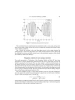
The comparison of the calculated and measured values of rotational speed, current, and
torque for starting state feeding by soft-starting (Figs. 2–4) and frequency starting devices
(Figs. 5–7) can be obser ved.
Verification Methods
Traditional methods
The traditional methods, which are used to measure induction machine parameters, are:
no-load test and short-circuit test. No-load test is useful for comparing the value of the
magnetizing current measured and that calculated. Specifically in low-powered machines
we focused on the problem of the air gap width estimation due to the effects of the cutting
process and its influence on the sheet borders. Because dynamic field-circuit models of
induction motors usually do not incorporate eddy currents, hysteresis, and mechanical
losses in the stator core, it is necessary to obtain experimentally only the magnetization
Figure 1. The gap region division.
II-12. Field-Circuit Finite Elements Models 277
-2
-1
0
1

2
3
4
5
6
0 0,1 0,2 0,3 0,4 0,5 0,6 0,7
measured
calculated
torque [Nm]
time [s]
Figure 2. Torque vs. time during soft-starting starting.
-5
-4
-3
-2
-1
0
1
2
3
4
5
0 0,1 0,2 0,3 0,4 0,5 0,6 0,7
current [A]
measured
c
alculated
time [s]
Figure 3. Comparison of calculated and measured current curves vs. time during soft starting.
0

200
400
600
800
1000
1200
1400
1600
1800
0 0,1 0,2 0,3 0,4 0,5 0,6 0,7 0,8
measured
calculated
speed [rpm]
time [s]
Figure 4. Comparison of calculated and measured speed curves vs. time during soft starting.
part of the no-load current. The quasi-static solvers calculate element permeability using
amplitude of the magnetic flux density. This can introduce some errors in highly saturated
small machinesdespite the transient calculation ofthe magnetization current needed[7-10].
In the presented motor, a comparison of measured and calculated values of the magnetizing
current is made. The second test concerns the shape of calculated and measured currents
at no-load. Comparing the shape of the two currents informs whether the flux distribution
in the different part of the examined motor is near to the real one. The maximum value
is mainly dependent on the air gap representation and saturation of the main parts of the
278 Kom
˛
eza et al.
-4
-2
0
2

4
6
8
0 0,05 0,1 0,15 0,2 0,25
measured
calculated
torque [Nm]
time [s]
Figure 5. Torque vs. time during frequency starting.
-4
-3
-2
-1
0
1
2
3
4
5
0 0,05 0,1 0,15 0,2 0,25
measured
calculated
current [A]
time [s]
Figure 6. Comparison of calculated and measured current curves vs. time during frequency starting.
0
200
400
600
800

1000
1200
1400
1600
1800
2000
0 0,05 0,1 0,15 0,2 0,25
measured
calculated
s
peed [rpm]
time [s]
Figure 7. Comparison of calculated and measured speed curves vs. time during frequency starting.
magnetic core. Fig. 8 shows the comparison of the current vs. time calculated with transient
and quasi-static solvers.
The results of comparison between two methods (AC and TR) and measurement are
summarized in Table 2.
The best results are obtained by TR method. It is very difficult in practice to obtain accu-
racy better then 5% especially for small power motors due to inaccuracies in the production
process and the results of the die-casting of the rotor cage and mechanical processing.
II-12. Field-Circuit Finite Elements Models 279
Table 2. The relative error between
calculation and measurement
Relative error
Phase A Phase B Phase C Average
AC
9,544 9,512 7,912 8,989
RT
3,535 8,524 8,376 6,812
Short-circuit test examines the accuracy of the leakage reactance estimation (end par ts

reactance are included as lumped parameters) and the skin effect in the rotor bars. The main
problem of the short-circuit test is the level of test current because of the local saturation
effects of the leakage fluxes. Therefore, if possible, only a test with a nominal voltage will
be really satisfactory. The measurement of the torque during thistest is very helpful (Fig. 9).
-1,5
-1
-0,5
0
0,5
1
1,5
0,1 0,11 0,12 0,13 0,14 0,15 0,16 0,17 0,18
time [s]
current [A]
measured
transient
steady-state
AC
Figure 8. Current vs. time curves for steady-state, transient calculation, and measurement.
calculated
0
1
2
3
4
5
6
0 50 100 150 200
current [A]
measured

voltage [V]
Figure 9. The short-circuit cur rent vs. voltage.
280 Kom
˛
eza et al.
Using the impulse DC supply test
Using this method we use the DC supply of one or two windings of the motor. With DC
impulse method it is possible to test many aspects of the motor’s behavior: the nonlinearity
of the main flux path, influence of saturation due to leakage flux of the windings and skin
effect of the currents induced in the rotor bar as well. Figs. 10 and 11 show the comparison
between the measured and calculated values of input current at different DC voltage value.
It is also possible to have a look on the classical equivalent circuit of the motor (Fig. 12).
0
0,5
1
1,5
2
2,5
3
3,5
0 0,02 0,04 0,06 0,08 0,1 0,12 0,14
calculated
measured
current [ A ]
time [ s ]
Figure 10. Current vs. time curves for DC supply at DC voltage value 63.05 V.
0
1
2
3

4
5
6
7
0 0,05 0,1
current [A]
0,15 0,2
calculated
times [s]
measured
Figure 11. Current vs. time curves for DC supply at DC voltage value 138 V.
R
s
U
s
L
s
L
M
R
R
L
R
Figure 12. The classical equivalent circuit of the motor.
II-12. Field-Circuit Finite Elements Models 281
Using the simplified, without current induced in stator and rotor cores, model of the
induction motor, the transfer function under linear condition is
Z(s) = R
s
+ sL

s
+
sL
m
(R
r
+ sL
r
)
R
r
+ s(L
r
+ L
m
)
(1)
When the DC impulse signal (step) is applied to the one phase terminals of the motor the
transient current response will be
I
s
(s) =
U
s
(s)
Z(s)
=
U
c
s


R
s
+ sL
s
+
sL
m
(R
r
+ sL
r
)
R
r
+ s(L
r
+ L
m
)

(2)
where U
c
is the value of applied DC voltage
I
s
(s) =
U
c

(R
r
+ s(L
r
+ L
m
))
s((R
s
+ sL
s
)(R
r
+ s(L
r
+ L
m
)) + sL
m
(R
r
+ sL
r
))
(3)
I
s
(s) =
U
c

(R
r
+ s(L
r
+ L
m
))
s(s − s
1
)(s − s
2
)(L
s
L
r
+ L
s
L
m
+ L
r
L
m
)
(4)
where s
1
and s
2
—simple poles of the current function are the roots of the equation

s
2
(L
s
L
r
+ L
s
L
m
+ L
r
L
m
) + s(R
s
L
r
+ R
s
L
m
+ R
r
L
s
+ R
r
L
m

) + R
s
R
r
= 0 (5)
The current vs. time function can be obtain using Heaviside’s formula
I
s
(t) = A
1
e
s
1
t
+ A
2
e
s
2
t
+ A
3
e
s
3
t
s
3
= 0 (6)
where

A
1
=
U
c
(R
r
+ s
1
(L
r
+ L
m
))
s
1
(s
1
− s
2
)(L
s
L
r
+ L
s
L
m
+ L
r

L
m
)
(7)
A
2
=
U
c
(R
r
+ s
2
(L
r
+ L
m
))
s
2
(s
2
− s
1
)(L
s
L
r
+ L
s

L
m
+ L
r
L
m
)
(8)
A
3
=
U
c
R
r
s
2
s
2
(L
s
L
r
+ L
s
L
m
+ L
r
L

m
)
=
U
c
R
s
(9)
When the time constant s
1
and s
2
differs significantly it is possible to separate them from
the measured current curve.
On the accuracy of the motor representation is shown by the values of the voltages
induced in open windings vs. time (Figs. 13 and 14).
Upon examining the obtained results it was obvious that separation of the current curve
exponential components would only be possible for small values of the instantaneous DC
current,for highervaluecurrent curve vs.time differs significantly from the curvedescribed
by equation (3) (Figs. 15–18).
The parameters calculated from measured curves are shown in Table 3.
Even when approximation was possible, the obtained values changed with voltage value.
Explanation of this result can be found easily by observing the field and current density
distributions calculated using field-circuit method.
In Figs. 19 and 20 the distribution of the relative permeability for DC voltage equals 138
V for two different time instances are shown.
282 Kom
˛
eza et al.
-8

-7
-6
-5
-4
-3
-2
-1
0
0 0,05 0,1 0,15 0,2
measured
calculated
times [s]voltage [V]
Figure 13. The voltage induced in open winding vs. time at DC voltage value 63.05 V.
-19
-17
-15
-13
-11
-9
-7
-5
-3
-1
1
0 0,05 0,1 0,15 0,2

calculated

measured
voltage [V]

times [s]
Figure 14. The voltage induced in open winding vs. time at DC voltage value 138 V.
0
0,1
0,2
0,3
0,4
0,5
0,6
0,7
0 0,06 0,09 0,12 0,15 0,18
time [s]
A1e
s1t
A2e
s2t
current [A]
calculated A
1e
s1t
+ A2e
s2t
measured
0,03
Figure 15. Decomposition of measured current curve vs. time into exponential components for DC
voltage 13.4 V.