SAS/ETS 9.22 User''''s Guide 43 ppt

412 ✦ Chapter 8: The AUTOREG Procedure
Printed Output
The AUTOREG procedure prints the following items:
1. the name of the dependent variable
2. the ordinary least squares estimates
3.
Estimates of autocorrelations, which include the estimates of the autocovariances, the autocor-
relations, and (if there is sufficient space) a graph of the autocorrelation at each LAG
4. if the PARTIAL option is specified, the partial autocorrelations
5.
the preliminary MSE, which results from solving the Yule-Walker equations. This is an
estimate of the final MSE.
6.
the estimates of the autoregressive parameters (Coefficient), their standard errors (Standard
Error), and the ratio of estimate to standard error (t Value)
7.
the statistics of fit for the final model. These include the error sum of squares (SSE), the
degrees of freedom for error (DFE), the mean square error (MSE), the mean absolute error
(MAE), the mean absolute percentage error (MAPE), the root mean square error (Root MSE),
the Schwarz information criterion (SBC), the Hannan-Quinn information criterion (HQC), the
Akaike information criterion (AIC), the corrected Akaike information criterion (AICC), the
Durbin-Watson statistic (Durbin-Watson), the regression
R
2
(Regress R-square), and the total
R
2
(Total R-square). For GARCH models, the following additional items are printed:
 the value of the log-likelihood function (Log Likelihood)
 the number of observations that are used in estimation (Observations)
 the unconditional variance (Uncond Var)

 the normality test statistic and its p-value (Normality Test and Pr > ChiSq)
8.
the parameter estimates for the structural model (Estimate), a standard error estimate (Standard
Error), the ratio of estimate to standard error (t Value), and an approximation to the significance
probability for the parameter being 0 (Approx Pr > |t|)
9.
If the NLAG= option is specified with METHOD=ULS or METHOD=ML, the regression
parameter estimates are printed again, assuming that the autoregressive parameter estimates are
known. In this case, the Standard Error and related statistics for the regression estimates will,
in general, be different from the case when they are estimated. Note that from a standpoint of
estimation, Yule-Walker and iterated Yule-Walker methods (NLAG= with METHOD=YW,
ITYW) generate only one table, assuming AR parameters are given.
10.
If you specify the NORMAL option, the Bera-Jarque normality test statistics are printed. If
you specify the LAGDEP option, Durbin’s h or Durbin’s t is printed.
ODS Table Names ✦ 413
ODS Table Names
PROC AUTOREG assigns a name to each table it creates. You can use these names to reference
the table when using the Output Delivery System (ODS) to select tables and create output data sets.
These names are listed in the Table 8.2.
Table 8.2 ODS Tables Produced in PROC AUTOREG
ODS Table Name Description Option
ODS Tables Created by the MODEL Statement
ClassLevels Class Levels default
FitSummary Summary of regression default
SummaryDepVarCen
Summary of regression (centered de-
pendent var)
CENTER
SummaryNoIntercept

Summary of regression (no intercept)
NOINT
YWIterSSE
Yule-Walker iteration sum of squared
error
METHOD=ITYW
PreMSE Preliminary MSE NLAG=
Dependent Dependent variable default
DependenceEquations Linear dependence equation
ARCHTest
Tests for ARCH disturbances based
on OLS residuals
ARCHTEST=
ARCHTestAR
Tests for ARCH disturbances based
on residuals
ARCHTEST=
(with NLAG=)
BDSTest BDS test for independence BDS<=()>
RunsTest Runs test for independence RUNS<=()>
TurningPointTest Turning Point test for independence TP<=()>
VNRRankTest
Rank version of von Neumann ratio
test for independence
VNRRANK<=()>
ChowTest Chow test and predictive Chow test
CHOW=
PCHOW=
Godfrey Godfrey’s serial correlation test GODFREY<=>
PhilPerron Phillips-Perron unit root test

STATIONARITY=
(PHILIPS<=()>)
(no regressor)
PhilOul Phillips-Ouliaris cointegration test
STATIONARITY=
(PHILIPS<=()>)
(has regressor)
ADF
Augmented Dickey-Fuller unit root
test
STATIONARITY=
(ADF<=()>) (no
regressor)
EngGran Engle-Granger cointegration test
STATIONARITY=
(ADF<=()>) (has
regressor)
ERS ERS unit root test
STATIONARITY=
(ERS<=()>)
414 ✦ Chapter 8: The AUTOREG Procedure
Table 8.2 continued
ODS Table Name Description Option
NgPerron Ng-Perron Unit root tests
STATIONARITY=
(NP=<()> )
KPSS
Kwiatkowski, Phillips, Schmidt, and
Shin test
STATIONARITY=

(KPSS<=()>)
ResetTest Ramsey’s RESET test RESET
ARParameterEstimates
Estimates of autoregressive parame-
ters
NLAG=
CorrGraph estimates of autocorrelations NLAG=
BackStep
Backward elimination of autoregres-
sive terms
BACKSTEP
ExpAutocorr Expected autocorrelations NLAG=
IterHistory Iteration history ITPRINT
ParameterEstimates Parameter estimates default
ParameterEstimatesGivenAR
Parameter estimates assuming AR pa-
rameters are given
NLAG=,
METHOD=
ULS | ML
PartialAutoCorr Partial autocorrelation PARTIAL
CovB Covariance of parameter estimates COVB
CorrB Correlation of parameter estimates CORRB
CholeskyFactor Cholesky root of gamma ALL
Coefficients
Coefficients for first NLAG observa-
tions
COEF
GammaInverse Gamma inverse GINV
ConvergenceStatus Convergence status table default

MiscStat
Durbin
t
or Durbin
h
, Bera-Jarque
normality test
LAGDEP=;
NORMAL
DWTest Durbin-Watson statistics DW=
ODS Tables Created by the RESTRICT Statement
Restrict Restriction table default
ODS Tables Created by the TEST Statement
FTest F test
default,
TYPE=ALL
WaldTest Wald test
TYPE=WALD|ALL
LMTest LM test
TYPE=LM|ALL
(only supported
with GARCH=
option)
LRTest LR test
TYPE=LR|ALL
(only supported
with GARCH=
option)
ODS Graphics ✦ 415
ODS Graphics

This section describes the use of ODS for creating graphics with the AUTOREG procedure.
To request these graphs, you must specify the ODS GRAPHICS statement. By default, only the
residual, predicted versus actual, and autocorrelation of residuals plots are produced. If, in addition
to the ODS GRAPHICS statement, you also specify the ALL option in either the PROC AUTOREG
statement or MODEL statement, all plots are created. For HETERO, GARCH, and AR models
studentized residuals are replaced by standardized residuals. For the autoregressive models, the
conditional variance of the residuals is computed as described in the section “Predicting Future
Series Realizations” on page 406. For the GA
RCH and HETERO models, residuals are assumed to have
h
t
conditional variance invoked by the
HT= option of the OUTPUT statement. For all these cases, the Cook’s D plot is not produced.
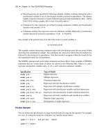
ODS Graph Names
PROC AUTOREG assigns a name to each graph it creates using ODS. You can use these names to
reference the graphs when using ODS. The names are listed in Table 8.3.
Table 8.3 ODS Graphics Produced by PROC AUTOREG
ODS Graph Name Plot Description Option
ACFPlot Autocorrelation of residuals ACF
FitPlot Predicted versus actual plot Default
CooksD Cook’s D plot ALL (no NLAG=)
IACFPlot Inverse autocorrelation of residuals ALL
QQPlot Q-Q plot of residuals ALL
PACFPlot Partial autocorrelation of residuals ALL
ResidualHistogram Histogram of the residuals ALL
ResidualPlot Residual plot Default
StudentResidualPlot Studentized residual plot ALL (no NLAG=/HETERO=/GARCH=)
StandardResidualPlot Standardized residual plot ALL
WhiteNoiseLogProbPlot Tests for white noise residuals ALL
416 ✦ Chapter 8: The AUTOREG Procedure

Examples: AUTOREG Procedure
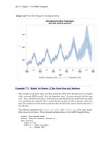
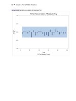
Example 8.1: Analysis of Real Output Series
In this example, the annual real output series is analyzed over the period 1901 to 1983 (Balke and
Gordon 1986, pp. 581–583). With the following DATA step, the original data are transformed using
the natural logarithm, and the differenced series DY is created for further analysis. The log of real
output is plotted in Output 8.1.1.
title 'Analysis of Real GNP';
data gnp;
date = intnx( 'year', '01jan1901'd, _n_-1 );
format date year4.;
input x @@;
y = log(x);
dy = dif(y);
t = _n_;
label y = 'Real GNP'
dy = 'First Difference of Y'
t = 'Time Trend';
datalines;
more lines
proc sgplot data=gnp noautolegend;
scatter x=date y=y;
xaxis grid values=('01jan1901'd '01jan1911'd '01jan1921'd '01jan1931'd
'01jan1941'd '01jan1951'd '01jan1961'd '01jan1971'd
'01jan1981'd '01jan1991'd);
run;
Example 8.1: Analysis of Real Output Series ✦ 417
Output 8.1.1 Real Output Series: 1901 – 1983
The (linear) trend-stationary process is estimated using the following form:
y
t

D ˇ
0
C ˇ
1
t C 
t
where

t
D 
t
 '
1

t1
 '
2

t2

t
IN.0; 

/
The preceding trend-stationary model assumes that uncertainty over future horizons is bounded since
the error term,

t
, has a finite variance. The maximum likelihood AR estimates from the statements
that follow are shown in Output 8.1.2:

proc autoreg data=gnp;
model y = t / nlag=2 method=ml;
run;
418 ✦ Chapter 8: The AUTOREG Procedure
Output 8.1.2 Estimating the Linear Trend Model
Analysis of Real GNP
The AUTOREG Procedure
Maximum Likelihood Estimates
SSE 0.23954331 DFE 79
MSE 0.00303 Root MSE 0.05507
SBC -230.39355 AIC -240.06891
MAE 0.04016596 AICC -239.55609
MAPE 0.69458594 HQC -236.18189
Durbin-Watson 1.9935 Regress R-Square 0.8645
Total R-Square 0.9947
Parameter Estimates
Standard Approx Variable
Variable DF Estimate Error t Value Pr > |t| Label
Intercept 1 4.8206 0.0661 72.88 <.0001
t 1 0.0302 0.001346 22.45 <.0001 Time Trend
AR1 1 -1.2041 0.1040 -11.58 <.0001
AR2 1 0.3748 0.1039 3.61 0.0005
Autoregressive parameters assumed given
Standard Approx Variable
Variable DF Estimate Error t Value Pr > |t| Label
Intercept 1 4.8206 0.0661 72.88 <.0001
t 1 0.0302 0.001346 22.45 <.0001 Time Trend
Nelson and Plosser (1982) failed to reject the hypothesis that macroeconomic time series are
nonstationary and have no tendency to return to a trend line. In this context, the simple random walk
process can be used as an alternative process:

y
t
D ˇ
0
C y
t1
C 
t
where 
t
D 
t
and y
0
D 0. In general, the difference-stationary process is written as
.L/.1  L/y
t
D ˇ
0
.1/ C Â.L/
t
where
L
is the lag operator. You can observe that the class of a difference-stationary process should
have at least one unit root in the AR polynomial .L/.1  L/.
The Dickey-Fuller procedure is used to test the null hypothesis that the series has a unit root in the
AR polynomial. Consider the following equation for the augmented Dickey-Fuller test:
y
t
D ˇ

0
C ıt C ˇ
1
y
t1
C
m
X
iD1

i
y
ti
C 
t
where
 D 1  L
. The test statistic


is the usual t ratio for the parameter estimate
O
ˇ
1
, but the


does not follow a t distribution.
Example 8.1: Analysis of Real Output Series ✦ 419
The following code performs the augmented Dickey-Fuller test with

m D 3
and we are interesting in
the test results in the linear time trend case since the previous plot reveals there is a linear trend.
proc autoreg data = gnp;
model y = / stationarity =(adf =3);
run;
The augmented Dickey-Fuller test indicates that the output series may have a difference-stationary
process. The statistic Tau with linear time trend has a value of
2:6190
and its p-value is
0:2732
.
The statistic Rho has a p-value of
0:0817
which also indicates the null of unit root is accepted at the
5% level. (See Output 8.1.3.)
Output 8.1.3 Augmented Dickey-Fuller Test Results
Analysis of Real GNP
The AUTOREG Procedure
Augmented Dickey-Fuller Unit Root Tests
Type Lags Rho Pr < Rho Tau Pr < Tau F Pr > F
Zero Mean 3 0.3827 0.7732 3.3342 0.9997
Single Mean 3 -0.1674 0.9465 -0.2046 0.9326 5.7521 0.0211
Trend 3 -18.0246 0.0817 -2.6190 0.2732 3.4472 0.4957
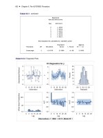
The AR(1) model for the differenced series DY is estimated using the maximum likelihood method
for the period 1902 to 1983. The difference-stationary process is written
y
t
D ˇ
0

C 
t

t
D 
t
 '
1

t1
The estimated value of
'
1
is
0:297
and that of
ˇ
0
is 0.0293. All estimated values are statistically
significant. The PROC step follows:
proc autoreg data=gnp;
model dy = / nlag=1 method=ml;
run;
The printed output produced by the PROC step is shown in Output 8.1.4.
420 ✦ Chapter 8: The AUTOREG Procedure
Output 8.1.4 Estimating the Differenced Series with AR(1) Error
Analysis of Real GNP
The AUTOREG Procedure
Maximum Likelihood Estimates
SSE 0.27107673 DFE 80

MSE 0.00339 Root MSE 0.05821
SBC -226.77848 AIC -231.59192
MAE 0.04333026 AICC -231.44002
MAPE 153.637587 HQC -229.65939
Durbin-Watson 1.9268 Regress R-Square 0.0000
Total R-Square 0.0900
Parameter Estimates
Standard Approx
Variable DF Estimate Error t Value Pr > |t|
Intercept 1 0.0293 0.009093 3.22 0.0018
AR1 1 -0.2967 0.1067 -2.78 0.0067
Autoregressive parameters assumed given
Standard Approx
Variable DF Estimate Error t Value Pr > |t|
Intercept 1 0.0293 0.009093 3.22 0.0018
Example 8.2: Comparing Estimates and Models
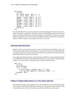
In this example, the Grunfeld series are estimated using different estimation methods. Refer to
Maddala (1977) for details of the Grunfeld investment data set. For comparison, the Yule-Walker
method, ULS method, and maximum likelihood method estimates are shown. With the DWPROB
option, the p-value of the Durbin-Watson statistic is printed. The Durbin-Watson test indicates the
positive autocorrelation of the regression residuals. The DATA and PROC steps follow:
Example 8.2: Comparing Estimates and Models ✦ 421
title 'Grunfeld''s Investment Models Fit with Autoregressive Errors';
data grunfeld;
input year gei gef gec;
label gei = 'Gross investment GE'
gec = 'Lagged Capital Stock GE'
gef = 'Lagged Value of GE shares';
datalines;
more lines

proc autoreg data=grunfeld;
model gei = gef gec / nlag=1 dwprob;
model gei = gef gec / nlag=1 method=uls;
model gei = gef gec / nlag=1 method=ml;
run;
The printed output produced by each of the MODEL statements is shown in Output 8.2.1 through
Output 8.2.4.