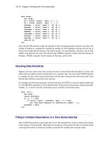
SAS/ETS 9.22 User''''s Guide 114 ppt

1122 ✦ Chapter 18: The MODEL Procedure
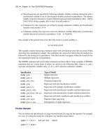
Figure 18.48 Static Estimation Results for Fish Model
The MODEL Procedure
Nonlinear OLS Parameter Estimates
Approx Approx
Parameter Estimate Std Err t Value Pr > |t|
ku 0.180159 0.0312 5.78 0.0044
ke 0.524661 0.1181 4.44 0.0113
To perform a dynamic estimation of the differential equation, add the DYNAMIC option to the FIT
statement.
proc model data=fish;
parm ku .3 ke .3;
dert.conc = ku - ke
*
conc;
fit conc / time = day dynamic;
run;
The equation DERT.CONC is integrated from
conc.0/ D 0
. The results from this estimation are
shown in Figure 18.49.
Figure 18.49 Dynamic Estimation Results for Fish Model
The MODEL Procedure
Nonlinear OLS Parameter Estimates
Approx Approx
Parameter Estimate Std Err t Value Pr > |t|
ku 0.167109 0.0170 9.84 0.0006
ke 0.469033 0.0731 6.42 0.0030
To perform a dynamic estimation of the differential equation and estimate the initial value, use the
following statements:
proc model data=fish;

parm ku .3 ke .3 conc0 0;
dert.conc = ku - ke
*
conc;
fit conc initial=(conc = conc0) / time = day dynamic;
run;
The INITIAL= option in the FIT statement is used to associate the initial value of a differential
equation with a parameter. The results from this estimation are shown in Figure 18.50.
Ordinary Differential Equations ✦ 1123
Figure 18.50 Dynamic Estimation with Initial Value for Fish Model
The MODEL Procedure
Nonlinear OLS Parameter Estimates
Approx Approx
Parameter Estimate Std Err t Value Pr > |t|
ku 0.164408 0.0230 7.14 0.0057
ke 0.45949 0.0943 4.87 0.0165
conc0 0.003798 0.0174 0.22 0.8414
Finally, to estimate the fish model by using the analytical solution, use the following statements:
proc model data=fish;
parm ku .3 ke .3;
conc = (ku/ ke)
*
( 1 -exp(-ke
*
day));
fit conc;
run;
The results from this estimation are shown in Figure 18.51.
Figure 18.51 Analytical Estimation Results for Fish Model
The MODEL Procedure

Nonlinear OLS Parameter Estimates
Approx Approx
Parameter Estimate Std Err t Value Pr > |t|
ku 0.167109 0.0170 9.84 0.0006
ke 0.469033 0.0731 6.42 0.0030
A comparison of the results among the four estimations reveals that the two dynamic estimations
and the analytical estimation give nearly identical results (identical to the default precision). The
two dynamic estimations are identical because the estimated initial value (0.00013071) is very close
to the initial value used in the first dynamic estimation (0). Note also that the static model did not
require an initial guess for the parameter values. Static estimation, in general, is more forgiving of
bad initial values.
The form of the estimation that is preferred depends mostly on the model and data. If a very accurate
initial value is known, then a dynamic estimation makes sense. If, additionally, the model can be
written analytically, then the analytical estimation is computationally simpler. If only an approximate
initial value is known and not modeled as an unknown parameter, the static estimation is less sensitive
to errors in the initial value.
1124 ✦ Chapter 18: The MODEL Procedure
The form of the error in the model is also an important factor in choosing the form of the estimation.
If the error term is additive and independent of previous error, then the dynamic mode is appropriate.
If, on the other hand, the errors are cumulative, a static estimation is more appropriate. See the
section “Monte Carlo Simulation” on page 1170 for an example.
Auxiliary Equations
Auxiliary equations can be used with differential equations. These are equations that need to be
satisfied with the differential equations at each point between each data value. They are automatically
added to the system, so you do not need to specify them in the SOLVE or FIT statement.
Consider the following example.
The Michaelis-Menten equations describe the kinetics of an enzyme-catalyzed reaction. The enzyme
is E, and S is called the substrate. The enzyme first reacts with the substrate to form the enzyme-
substrate complex ES, which then breaks down in a second step to form enzyme and products
P.

The reaction rates are described by the following system of differential equations:
d ŒES
dt
D k
1
.ŒE  ŒES/ŒS  k
2
ŒES  k
3
ŒES
d ŒS
dt
D k
1
.ŒE  ŒES/ŒS C k
2
ŒES
[E] D ŒE
tot
 ŒES
The first equation describes the rate of formation of ES from E + S. The rate of formation of ES from
E + P is very small and can be ignored. The enzyme is in either the complexed or the uncomplexed
form. So if the total (
ŒE
tot
) concentration of enzyme and the amount bound to the substrate is
known, ŒE can be obtained by conservation.
In this example, the conservation equation is an auxiliary equation and is coupled with the differential
equations for integration.
Time Variable

You must provide a time variable in the data set. The name of the time variable defaults to TIME.
You can use other variables as the time variable by specifying the TIME= option in the FIT or
SOLVE statement. The time intervals need not be evenly spaced. If the time variable for the current
observation is less than the time variable for the previous observation, the integration is restarted.
Ordinary Differential Equations ✦ 1125
Differential Equations and Goal Seeking
Consider the following differential equation
y
0
D ax
and the data set
data t2;
y=0; time=0; output;
y=2; time=1; output;
y=3; time=2; output;
run;
The problem is to find values for X that satisfy the differential equation and the data in the data set.
Problems of this kind are sometimes referred to as goal-seeking problems because they require you
to search for values of X that satisfy the goal of Y.
This problem is solved with the following statements:
proc model data=t2;
independent x 0;
dependent y;
parm a 5;
dert.y = a
*
x;
solve x / out=goaldata;
run;
proc print data=goaldata;

run;
The output from the PROC PRINT statement is shown in Figure 18.52.
Figure 18.52 Dynamic Solution
Obs _TYPE_ _MODE_ _ERRORS_ x y time
1 PREDICT SIMULATE 0 0.0 0 0
2 PREDICT SIMULATE 0 0.8 2 1
3 PREDICT SIMULATE 0 -0.4 3 2
Note that an initial value of 0 is provided for the X variable because it is undetermined at TIME = 0.
In the preceding goal-seeking example, X is treated as a linear function between each set of data
points (see Figure 18.53).
1126 ✦ Chapter 18: The MODEL Procedure
Figure 18.53 Form of X Used for Integration in Goal Seeking
If you integrate y
0
D ax manually, you have
x.t / D
t
f
 t
t
f
 t
o
x
o
C
t  t
o
t
f

 t
o
x
f
y
f
 y
o
D
Z
t
f
t
o
ax.t/ dt
D a
1
t
f
 t
o
.t.t
f
x
o
 t
o
x
f
/ C

1
2
t
2
.x
f
 x
o
//
ˇ
ˇ
ˇ
ˇ
t
f
t
o
For observation 2, this reduces to
y
f
 y
o
D
1
2
ax
f
2 D 2:5x
f
So x D 0:8 for this observation.

Goal seeking for the TIME variable is not allowed.
Restrictions and Bounds on Parameters
Using the BOUNDS and RESTRICT statements, PROC MODEL can compute optimal estimates
subject to equality or inequality constraints on the parameter estimates.
Restrictions and Bounds on Parameters ✦ 1127
Equality restrictions can be written as a vector function:
h.Â/ D 0
Inequality restrictions are either active or inactive. When an inequality restriction is active, it is
treated as an equality restriction. All inactive inequality restrictions can be written as a vector
function:
F .Â/  0
Strict inequalities, such as
.f .Â/ > 0/
, are transformed into inequalities as
f .Â/ .1 /    0
,
where the tolerance

is controlled by the EPSILON= option in the FIT statement and defaults to
10
8
. The ith inequality restriction becomes active if
F
i
< 0
and remains active until its Lagrange
multiplier becomes negative. Lagrange multipliers are computed for all the nonredundant equality
restrictions and all the active inequality restrictions.
For the following, assume the vector
h.Â/

contains all the current active restrictions. The constraint
matrix A is
A.
O
Â/ D
@h.
O
Â/
@
O
Â
The covariance matrix for the restricted parameter estimates is computed as
Z.Z
0
HZ/
1
Z
0
where
H
is Hessian or approximation to the Hessian of the objective function (
.X
0
.diag.S/
1
˝I/X/
for OLS), and
Z
is the last
.np nc/

columns of
Q
.
Q
is from an LQ factorization of the constraint
matrix, nc is the number of active constraints, and np is the number of parameters. See Gill, Murray,
and Wright (1981) for more details on LQ factorization. The covariance column in Table 18.2
summarizes the Hessian approximation used for each estimation method.
The covariance matrix for the Lagrange multipliers is computed as
.AH
1
A
0
/
1
The p-value reported for a restriction is computed from a beta distribution rather than a t distribution
because the numerator and the denominator of the t ratio for an estimated Lagrange multiplier are
not independent.
The Lagrange multipliers for the active restrictions are printed with the parameter estimates. The
Lagrange multiplier estimates are computed using the relationship
A
0
 D g
where the dimensions of the constraint matrix
A
are the number of constraints by the number of
parameters,

is the vector of Lagrange multipliers, and g is the gradient of the objective function at
the final estimates.

The final gradient includes the effects of the estimated
S
matrix. For example, for OLS the final
gradient would be:
g D X
0
.diag.S/
1
˝I/r
where r is the residual vector. Note that when nonlinear restrictions are imposed, the convergence
measure R might have values greater than one for some iterations.
1128 ✦ Chapter 18: The MODEL Procedure
Tests on Parameters
In general, the hypothesis tested can be written as
H
0
W h.Â/ D 0
where
h.Â/
is a vector-valued function of the parameters
Â
given by the r expressions specified on
the TEST statement.
Let
O
V
be the estimate of the covariance matrix of
O
Â
. Let

O
Â
be the unconstrained estimate of
Â
and
Q
Â
be the constrained estimate of  such that h.
Q
Â/ D 0. Let
A.Â/ D @h.Â/=@Â j
O
Â
Let r be the dimension of
h.Â/
and n be the number of observations. Using this notation, the test
statistics for the three kinds of tests are computed as follows.
The Wald test statistic is defined as
W D h
0
.
O
Â/
8
:
A.
O
Â/
O
VA

0
.
O
Â/
9
;
1
h.
O
Â/
The Wald test is not invariant to reparameterization of the model (Gregory and Veall 1985; Gallant
1987, p. 219). For more information about the theoretical properties of the Wald test, see Phillips
and Park (1988).
The Lagrange multiplier test statistic is
R D 
0
A.
Q
Â/
Q
VA
0
.
Q
Â/
where  is the vector of Lagrange multipliers from the computation of the restricted estimate
Q
Â.
The Lagrange multiplier test statistic is equivalent to Rao’s efficient score test statistic:
R D .@L.

Q
Â/=@Â/
0
Q
V.@L.
Q
Â/=@Â/
where
L
is the log-likelihood function for the estimation method used. For SUR, 3SLS, GMM, and
iterated versions of these methods, the likelihood function is computed as
L D Objective Nobs=2
For OLS and 2SLS, the Lagrange multiplier test statistic is computed as:
R D Œ.@
O
S.
Q
Â/=@Â/
0
Q
V.@
O
S.
Q
Â/=@Â/=
O
S.
Q
Â/
where

O
S.
Q
Â/ is the corresponding objective function value at the constrained estimate.
The likelihood ratio test statistic is
T D 2

L.
O
Â/ L.
Q
Â/
Á
where
Q
 represents the constrained estimate of  and L is the concentrated log-likelihood value.
Hausman Specification Test ✦ 1129
For OLS and 2SLS, the likelihood ratio test statistic is computed as:
T D .n  nparms/ .
O
S.
Q
Â/ 
O
S.
O
Â//=
O
S.
O

Â/
This test statistic is an approximation from
T D n  log
Â
1 C
rF
n  nparms
Ã
when the value of rF=.n nparms/ is small (Greene 2004, p. 421).
The likelihood ratio test is not appropriate for models with nonstationary serially correlated errors
(Gallant 1987, p. 139). The likelihood ratio test should not be used for dynamic systems, for systems
with lagged dependent variables, or with the FIML estimation method unless certain conditions are
met (see Gallant 1987, p. 479).
For each kind of test, under the null hypothesis the test statistic is asymptotically distributed as a

2
random variable with r degrees of freedom, where r is the number of expressions in the TEST
statement. The p-values reported for the tests are computed from the

2
.r/
distribution and are only
asymptotically valid. When both RESTRICT and TEST statements are used in a PROC MODEL
step, test statistics are computed by taking into account the constraints imposed by the RESTRICT
statement.
Monte Carlo simulations suggest that the asymptotic distribution of the Wald test is a poorer
approximation to its small sample distribution than the other two tests. However, the Wald test has
the least computational cost, since it does not require computation of the constrained estimate
Q
Â.

The following is an example of using the TEST statement to perform a likelihood ratio test for a
compound hypothesis.
test a
*
exp(-k) = 1-k, d = 0 ,/ lr;
It is important to keep in mind that although individual t tests for each parameter are printed by
default into the parameter estimates table, they are only asymptotically valid for nonlinear models.
You should be cautious in drawing any inferences from these t tests for small samples.
Hausman Specification Test
Hausman’s specification test, or m-statistic, can be used to test hypotheses in terms of bias or
inconsistency of an estimator. This test was also proposed by Wu (1973). Hausman’s m-statistic is as
follows.
Given two estimators,
O
ˇ
0
and
O
ˇ
1
, where under the null hypothesis both estimators are consistent but
only
O
ˇ
0
is asymptotically efficient and under the alternative hypothesis only
O
ˇ
1
is consistent, the

m-statistic is
m D Oq
0
.
O
V
1

O
V
0
/

Oq
1130 ✦ Chapter 18: The MODEL Procedure
where
O
V
1
and
O
V
0
represent consistent estimates of the asymptotic covariance matrices of
O
ˇ
1
and
O
ˇ

0
respectively, and
q D
O
ˇ
1

O
ˇ
0
The m-statistic is then distributed

2
with
k
degrees of freedom, where
k
is the rank of the matrix
.
O
V
1

O
V
0
/. A generalized inverse is used, as recommended by Hausman and Taylor (1982).
In the MODEL procedure, Hausman’s m-statistic can be used to determine if it is necessary to use an
instrumental variables method rather than a more efficient OLS estimation. Hausman’s m-statistic can
also be used to compare 2SLS with 3SLS for a class of estimators for which 3SLS is asymptotically

efficient (similarly for OLS and SUR).
Hausman’s m-statistic can also be used, in principle, to test the null hypothesis of normality when
comparing 3SLS to FIML. Because of the poor performance of this form of the test, it is not offered
in the MODEL procedure. See Fair (1984, pp. 246–247) for a discussion of why Hausman’s test
fails for common econometric models.
To perform a Hausman’s specification test, specify the HAUSMAN option in the FIT statement. The
selected estimation methods are compared using Hausman’s m-statistic.
In the following example, Hausman’s test is used to check the presence of measurement error. Under
H
0
of no measurement error, OLS is efficient, while under
H
1
, 2SLS is consistent. In the following
code, OLS and 2SLS are used to estimate the model, and Hausman’s test is requested.
proc model data=one out=fiml2;
endogenous y1 y2;
y1 = py2
*
y2 + px1
*
x1 + interc;
y2 = py1
*
y1 + pz1
*
z1 + d2;
fit y1 y2 / ols 2sls hausman;
instruments x1 z1;
run;

The output specified by the HAUSMAN option produces the results shown in Figure 18.54.
Figure 18.54 Hausman’s Specification Test Results
The MODEL Procedure
Hausman's Specification Test Results
Efficient Consistent
under H0 under H1 DF Statistic Pr > ChiSq
OLS 2SLS 6 13.86 0.0313
Figure 18.54 indicates that 2SLS is preferred over OLS at 5% level of significance. In this case, the
null hypothesis of no measurement error is rejected. Hence, the instrumental variable estimator is
required for this example due to the presence of measurement error.
Chow Tests ✦ 1131
Chow Tests
The Chow test is used to test for break points or structural changes in a model. The problem is posed
as a partitioning of the data into two parts of size n
1
and n
2
. The null hypothesis to be tested is
H
o
W ˇ
1
D ˇ
2
D ˇ
where
ˇ
1
is estimated by using the first part of the data and
ˇ

2
is estimated by using the second part.
The test is performed as follows (see Davidson and MacKinnon 1993, p. 380).
1. The p parameters of the model are estimated.
2.
A second linear regression is performed on the residuals,
Ou
, from the nonlinear estimation in
step one.
Ou D
O
Xb Cresiduals
where
O
X
is Jacobian columns that are evaluated at the parameter estimates. If the estimation
is an instrumental variables estimation with matrix of instruments
W
, then the following
regression is performed:
Ou D P
W

O
Xb Cresiduals
where P
W

is the projection matrix.
3.

The restricted SSE (RSSE) from this regression is obtained. An SSE for each subsample is
then obtained by using the same linear regression.
4. The F statistic is then
f D
.RSSE  SSE
1
 SSE
2
/=p
.SSE
1
C SSE
2
/=.n  2p/
This test has p and n  2p degrees of freedom.
Chow’s test is not applicable if
min.n
1
; n
2
/ < p
, since one of the two subsamples does not contain
enough data to estimate
ˇ
. In this instance, the predictive Chow test can be used. The predictive
Chow test is defined as
f D
.RSSE  SSE
1
/.n

1
 p/
SSE
1
n
2
where
n
1
> p
. This test can be derived from the Chow test by noting that the
SSE
2
D 0
when
n
2
<D p and by adjusting the degrees of freedom appropriately.
You can select the Chow test and the predictive Chow test by specifying the CHOW=arg and the
PCHOW=arg options in the FIT statement, where arg is either the number of observations in the
first sample or a parenthesized list of first sample sizes. If the size of the one of the two groups in
which the sample is partitioned is less than the number of parameters, then a predictive Chow test is
automatically used. These tests statistics are not produced for GMM and FIML estimations.
The following is an example of the use of the Chow test.