The Complete IS-IS Routing Protocol- P6 ppsx

}
interface lo0.0;
}
}
JUNOS displays the Hello timers in millisecond resolution using the show isis
interface detail operational level command.
JUNOS command output
hannes@Frankfurt> show isis interface detail
IS-IS interface database:
so-0/1/2.0
Index: 67, State: 0x6, Circuit id: 0x1, Circuit type: 3
LSP interval: 100 ms, CSNP interval: 5 s
Level Adjacencies Priority Metric Hello (s) Hold (s) Designated
Router
1 1 64 10 0.333 1
2 1 64 10 0.333 1
The JUNOS interface multiplier is hard coded (meaning it cannot be changed) to a
value of 3. A hold-timer of 1 second therefore results in a Hello interval of 333 ms, which
is the lowest Hello interval possible on JUNOS.
Relying on Hellos puts an upper boundary of 1 second to the detection time following
a link-failure on the routing protocols. But by tracking an interface state, routers can
detect the liveliness state much more quickly.
5.6.2 Interface Tracking
The chipsets that drive modern router interfaces report link errors, such as a loss of
signal, to the routing sub-system within a few milliseconds. For high-speed detection,
therefore, optical interfaces are the best choice. However, there are still similar prob-
lems, as illustrated in Figure 5.10. If there are active elements in the middle of the trans-
mission chain, then local errors are not propagated downstream and the receiving router
does not detect that the light went out.
SONET/SDH offers a true advantage over other physical media like Ethernet, which
do not propagate local errors to downstream Network Elements.

Many Protocols like Frame Relay and ATM also include their own Local Management
Interface (LMI) protocol which performs link-layer keep-alive checking, and so on.
Unfortunately there is still no LMI-like protocol for Ethernet. Bi-directional fault detec-
tion attempts make a neutral liveliness-checking protocol available.
5.6.3 Bi-directional Fault Detection (BFD)
BFD is defined in draft-katz-ward-bfd-01, and its encoding rules are documented in
draft-katz-ward-bfd-v4v6-1hop-00. BFD is an answer to the following problems:
•
Link-Layer neutral high frequency keep-alive protocol
•
Offload high frequency keep-alive processing from the IGP Layer
Neighbour Liveliness Detection 137
138 5. Neighbour Discovery and Handshaking
•
Support sub-second timers on behalf of protocols that cannot
•
Negotiate timers dynamically
The BFD protocol, unlike many other protocols, includes no auto-neighbour discov-
ery. It has client software instead, typical of the IP routing protocols, and based on the
detected IGP neighbours. The IGP asks the BFD module to set up a BFD session to the
Link IP addresses of the provided neighbours.
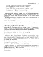
BFD is (at time of writing this book) only available for JUNOS. The first release with
support for BFD is JUNOS 6.1 onwards. The configuration of BFD is a property of the
interface {} stanza inside the protocols isis {} branch.
JUNOS configuration
Under the bfd-liveness-detection stanza you can configure the minimum transmit
interval plus the detection-time multiplier.
protocols {
isis {
interface so-1/2/0.0 {

bfd-liveness-detection {
minimum-interval 100;
multiplier 5;
}
}
[… ]
interface lo0.0;
}
}
In this example the router emits Hello packets at a rate of once every 100 ms. If the
neighbour does not receive BFD control packets for 500 ms, this router can declare the
origniator dead and move to an interface down state in the FSM.
BFD runs on top of IP UDP port 3784 and 3785. Port 3784 is used for control packets
and 3785 is used for Echo Mode traffic. The JUNOS implementation just supports con-
trol packets for liveliness detection. Echo Mode is envisioned for the future: the plan is
that forwarding plane software can generate that traffic and the control plane is only
needed for parameter setup.
The following Tcpdump output shows the parameters that are conveyed using the
24-bytes fixed length packet.
Tcpdump output
The BFD protocol runs on top of UDP port 3784 and 3785. It is meant as a high frequency
keep-alive mechanism which augments routing protocols that do not have sub-second
timer support.
09:32:30.884968 IP 172.16.223.236.3784 > 172.16.223.235.3784: BFDv0,
length: 24
Control, Flags: [I Hear You], Diagnostic: Control Detection
Time Expired (0x01)
Detection Timer Multiplier: 5 (500 ms Detection time),
BFD Length: 24
My Discriminator: 0x00000001, Your Discriminator: 0x00000002

Desired min Tx Interval: 100 ms
Required min Rx Interval: 200 ms
Required min Echo Interval: 0 ms
Session state transactions are provided using the Flag contents. The Desired/
Required Timer Fields are used for negotiating a common timer that both peers can
accept. The pair of discriminators is necessary to multiplex several sessions between a
pair of hosts.
After BFD has been enabled on both sides, one can verify if a BFD-capable neighbour
has been found on the other end and if the BFD session is Up. The show bfd ses-
sion command displays the session state.
JUNOS command output
Using the show bfd session command you can display the current state and details of
the active BFD sessions.
hannes@Frankfurt> show bfd session extensive
Transmit
Address State Interface Detect Time Interval Multiplier
172.16.223.236 Up so-0/1/2.0 1.000 0.100 5
Client ISIS L1, TX interval 0.100, RX interval 0.100, multiplier 5
Client ISIS L2, TX interval 0.100, RX interval 0.100, multiplier 5
Session up time 12:34:22, previous down time 00:00:06
Local diagnostic CtlExpire, remote diagnostic None
Remote heard, hears us
Min async interval 0.100, min slow interval 1.000
Adaptive async tx interval 0.100, rx interval 0.200
Local min tx interval 0.100, min rx interval 0.100, multiplier 5
Remote min tx interval 0.100, min rx interval 0.100, multiplier 5
Local discriminator 1, remote discriminator 2
Echo mode disabled/inactive
1 sessions, 2 clients
Cumulative transmit rate 10.0 pps, cumulative receive rate 5.0 pps

BFD is likely to become the dominant keep-alive protocol due its open implemen-
tation. It is expected to even be the protocol of choice between routers and servers.
For server applications like voice-over IP or financial applications there are open-source
BFD implementations for hosts available.
Neighbour Liveliness Detection 139
5.7 Summary
IS-IS adjacency processing has changed over the years. It started out with simple 2-way
finite state machines and, due to the underlying problems of not detecting half-broken
links, it quickly evolved to a 3-way FSM. It is remarkable that the defects of the under-
lying protocol have been solved with just the addition of an optional Adjacency State
TLV. Reliably detecting that a neighbour is Up or Down is not enough for today’s ser-
vice provider environments. On the one hand the implementation has to be slow enough
to protect the network from flapping adjacencies that are propagated through the network –
on the other hand there is a need for quick keep-alive detection mechanisms. Due to the
rise of Ethernet as popular core-facing interface technology, an LMI-like protocol like
Bi-directional Fault Detection (BFD) had to be designed. The application of BFD to
serve as an IGP detection protocol is just the start. It is expected that BFD will be used
for other network protocols or other environments like application keep-alive detection
for mission-critical servers.
140 5. Neighbour Discovery and Handshaking
6
Generating, Flooding and Ageing LSPs
141
Unlike distance vector protocols, such as RIP, link-state routing protocols, such as OSPF
and IS-IS, don’t tell only their neighbours about the topology of the network. Link-state
protocols distribute both their IP reachability and topological view far beyond their adja-
cent neighbours, ultimately flooding this information to all routers in an area.
To keep the reachability information in the network current, link-state protocols need
to have a basic set of functions available that can be used to originate, distribute and
finally revoke, or time-out topology information. In IS-IS-speak, that piece of topology

information is encoded in a link-state protocol data unit (LSP). This chapter covers these
functions and the surrounding network events th at cause the IS-IS protocol to generate,
flood and finally age LSPs.
Link-state routing protocols such as IS-IS follow a paradigm that can best be described
as distributed databases with local computation, which is quite different to the way other
common routing protocols like RIP and BGP work. Distributed databases are discussed
in more detail in the following section.
6.1 Distributed Databases
Before explaining how a distributed database works, first consider what a localized data-
base looks like and how routing protocols use it. Localized databases mean that every
router has its own local view of the network and does not know the exact topology of the
network as a whole. This is like a tourist in a foreign city having no clue about what the
overall topology of the city (the street layout) looks like. All the tourist has is a local view
of the places and streets that are next to the tourist’s immediate location. This makes it
very difficult to find the best path to a landmark or museum, and in the worst case situation,
the tourist has to try out several paths, being careful not to circle around the same locations.
Localized databases work the same way. In contrast, a distributed database approach
works differently: here all of the routers share common information about what the network
looks like. If the tourist in the example has got lost, a distributed database map would give
them a more complete map of the best way to get to a particular destination in the city (or
in this case, the network).
How does IS-IS compute the map of the network? If each router just contributes its
local view to its neighbours, and if that information can be shared among all the routers
in a network, then each will ultimately have a global map of the network. Link-state rout-
ing protocols, such as IS-IS, work like a jigsaw puzzle, as shown in Figure 6.1. Each
router in the figure represents one piece of the puzzle, and if all of the puzzle pieces are
present, then each router can start to put the puzzle together to acquire an understanding
of what the big picture looks like. The collection of puzzle pieces is called the link-state
database. IS-IS has a number of techniques called flooding and synchronizing to get a
complete map of the network. In this chapter, you will learn about the individual puzzle

pieces, which are called link-state protocol data units (LSPs), and how IS-IS distributes
the information they contain.
IS-IS, by default, tries to acquire two maps from its neighbours and therefore maintains
two databases to store topology-related information. Information for the first map, which
typically represents the topology inside the close collection of routers, called a point-
of-presence (POP), is stored in the Level 1 (L1) database. Sticking with the lost tourist
example, think of this as just a local map that guides you around the next few streets. The
second map, which typically represents the backbone structure of the network, is stored
142 6. Generating, Flooding and Ageing LSPs
Pennsauken
Frankfurt
London
Washington
NewYork
Paris
FIGURE 6.1. A distributed link-state database is like a jigsaw puzzle
Distributed Databases 143
in the Level 2 (L2) database. This would best compare to a nationwide map where all the
freeways and highways are shown. You can take a quick look into both of these link-state
databases to find out exactly which puzzle pieces the database holds by issuing a show
isis database command on both the IOS and JUNOS software platforms.
IOS command output
The contents of the IS-IS link-state database can be displayed using the show isis
database command:
Amsterdam# show isis database
[… ]
IS-IS Level-1 Link State Database:
LSPID LSP Seq Num LSP Checksum LSP Holdtime ATT/P/OL
New-York.00-00 0x00002fac 0xC24F 60128 1/0/0
[… ]

IS-IS Level-2 Link State Database:
LSPID LSP Seq Num LSP Checksum LSP Holdtime ATT/P/OL
LINX-gw.00-00 0x00000128 0xB8EF 36163 0/0/1
LINX-gw.01-00 0x00000128 0x455A 42001 0/0/0
VIX-gw.00-00 0x00000123 0xEFC1 5023 0/0/0
[… ]
The output shows you one “puzzle piece” of information in each line. Each LSP is
uniquely identified by its LSP-ID. The exact format of the LSP-ID will be discussed later
in this chapter. All that is important for now is that it says something about the router that
originated that LSP. The sequence number is a kind of version field that tells receivers
which information is more recent. The checksum enables to check at the receiver if the
LSP has been corrupted during its long way through the network. Finally, hold-time and
the ATT/P/OL gives some information about the validity of that information and how
long it will be valid, and just like a passport it has an expiration date.
JUNOS command output
In the JUNOS software, you can display the IS-IS database using the show isis data-
base command. Watch for an inconsistency between the LSPs being sent and received,
as this is a problem indication:
hannes@New-York> show isis database
IS-IS level 1 link-state database:
LSP ID Sequence Checksum Lifetime Attributes
New-York.00-00 0x2fac 0xc24f 62063 L1 Attached
[… ]
4 LSPs
IS-IS level 2 link-state database:
LSP ID Sequence Checksum Lifetime Attributes
LINX-gw.00-00 0x128 0xb8ef 36063 L1 L2 Overload
LINX-gw.01-00 0x128 0x455a 41901 L1 L2
VIX-gw.00-00 0x123 0xefc1 4922 L1 L2
[… ]

12 LSPs
The JUNOS software output contains similar information to the IOS software output.
The only difference is the little bit more detailed breakdown of the so-called attribute
typeblock, which will be discussed later in this chapter. As far as the attribute typeblock
is concerned, the JUNOS output is more verbose than the IOS equivalent.
Based on the information in the two link-state databases for L1 and L2, each router in
an IS-IS network computes the topology of the network independently of every other
router. This principle of independent router operation is called local computation. This is
the topic of the next discussion.
6.2 Local Computation
Routing protocols, such as RIP or BGP, compute the best path through a network in a dis-
tributed fashion. That is, no single RIP or BGP router knows what the other routers know
about the route, and this is a real limitation. For instance, each time a RIP router passes on
a route to its neighbour, the route gets a worse value. This “worseness” is indicted in a
metric field, which represents the hop-count (number of routers) that a router is away from
the router attached to the source sub-net. In Figure 6.2 the sub-net 192.168.1/24 is directly
connected to RIP Router #1. Router #1 reports the sub-net to its neighbours with a hop
count of 1. Router #2 learns the sub-net with a metric of 1 and reports it further to the right
side of the figure after incrementing the metric field by one. The routing update therefore
arrives at Router #3 with a metric of 2. But Router #1 has no idea what value this route has
on Router #3. RIP routing illustrates how a distributed computation scheme works.
IS-IS utilizes a totally different way of calculating routing information. Before the route
calculation takes place, all IS-IS routers distribute the information about the local views
of the routers to each other. Intermediate routers along the way must not change these
views (represented in the LSPs). After this distribution (flooding), a common route-
calculation scheme, which in IS-IS is called the shortest path first (SPF) algorithm, is
applied. Note that each router computes the routes independently from every other router.
144 6. Generating, Flooding and Ageing LSPs
192.168.1/24
…

RIP Router 1 RIP Router 2 RIP Router 3 RIP Router 4
192.168.1/24 (1) 192.168.1/24 (2) 192.168.1/24 (3)
…
192.168.1/24 (4)
…
…
FIGURE 6.2. RIP calculates the metric in a distributed fashion
Local Computation 145
You can watch the result of the SPF calculation by issuing a show ip route isis com-
mand on IOS platforms and a show isis route command on Juniper Network routers.
In IOS, you cannot see the entire results of the SPF calculation – all you can see are
the results that make it into the main routing table. That excludes redundant routers that
happen to be in both IS-IS levels. The IS-IS learned routes that are active in the routing
table can be displayed using the show ip route isis command.
IOS command output
Amsterdam#show ip route isis
[… ]
i L1 192.168.0.55 [115/10] via 172.16.144.2, POS3/0
i L1 192.168.0.57 [115/10] via 172.16.144.2, POS4/0
i L2 192.168.1.122 [115/10] via 172.16.177.18, GigabitEthernet3/0
[… ]
The output tells us basically what routes (second column) did get installed in the local
routing and forwarding tables. Each line contains information about a single route. The
first column shows the level. The numbers in the brackets after the route give informa-
tion about the weight or, as it is called in Cisco IOS speak, the administrative distance of
the routing protocol that inserted this route into the routing table (in this case, IS-IS).
After the “via” statement the IP address of a locally connected router appears (the next-
hop). Finally the end of each line gives the physical interface through which the next-hop
can be reached and this is how packets to this destination will leave the router.
In the JUNOS software, you can display both the immediate results from the SPF calcu-

lation as well as the routes installed in the routing table. The SPF results are displayed using
the show isis route command. The IS-IS learned routes that are active in the main
routing table can be displayed using the show route protocol isis command.
JUNOS software command output
hannes@Pennsauken> show isis route
IS-IS routing table Current version: L1: 0 L2: 485
Prefix L Version Metric Type Interface Via
172.16.44.248/30 2 485 61770 int so-3/0/0.0 London
192.168.49.5/32 2 485 67850 int so-3/0/0.0 London
192.168.49.67/32 2 485 67860 int so-3/0/0.0 London
192.168.52.177/32 2 485 127850 int so-3/0/0.0 Frankfurt
192.168.54.164/32 2 485 128510 int so-3/0/0.0 Frankfurt
172.16.176.0/24 2 485 121770 int so-3/0/0.0 Frankfurt
172.16.176.32/30 2 485 127830 int so-3/0/0.0 New-York
172.16.176.60/30 2 485 123790 int so-3/0/0.0 New-York
[… ]
The format of the output is one route entry per line. The first column contains the route
and the second column contains information about the level where this route did result
from. The version field is just an internal number that tells you how the SPF run number
based upon this route was calculated. The version field is typically not interesting in
troubleshooting networks. The metric tells the distance relative to the local router of the
prefix. Next is an indication whether the route is internal or external. Typically all the
routes are internal unless routes have been injected from other routing protocols into the IS-
IS database. Finally, the interface where the traffic leaves the router is displayed, plus the
forwarding router’s name.
JUNOS software command output
hannes@Pennsauken> show route protocol isis
inet.0: 118243 destinations, 246129 routes (118243 active,
0 holddown, 0 hidden)
+ = Active Route, - = Last Active, * = Both

172.16.44.248/30 *[IS-IS/18] 4d 12:57:11, metric 41550, tag 2
> to 172.16.5.93 via so-3/2/0.0
192.168.49.5/32 *[IS-IS/18] 2d 07:26:54, metric 67850, tag 2
> to 172.16.5.93 via so-2/3/0.0
192.168.49.67/32 *[IS-IS/18] 1d 20:01:28, metric 67860, tag 2
> to 172.16.5.93 via so-7/0/0.0
[… ]
In the show route protocol isis output we can see a subset of routes that got
displayed in show isis routes. Those are the routes that competed for installation in
the routing table with other routing protocols that may have had similar information;
however, the routes in this table are the ones that have won. In JUNOS the level of routes
is displayed in the tag field – a tag 2 means that this is a Level 2 route. The number in the
brackets is a similar value to the administrative distance for IOS platforms, called sim-
ply the route preference. The to and via keywords indicate the next-hop and the outgoing
interface.
The universal transport vehicle to build the IS-IS database map is called a link-state
protocol data unit or LSP for short, which is another OSI-speak word for link-state
packet. In the following sections, you will see what information an LSP contains, how
the LSP gets distributed, and how LSPs get throttled when the network is busy.
6.3 LSPs and Revision Control
The information element that transports IS-IS-related information to populate all the
routers’ link-state databases is called the link-state PDU or LSP. Each router in an IS-IS
network generates at least one LSP that describes, as the name implies, the current state
of the links to other routers. Actually, an LSP conveys more than just the state of the links
or circuits on the router. Routers use LSPs as a kind of envelope to get different types of
information elements such as IP routes, checksums and even router names across to other
routers. LSPs need to be accurate and up-to-date. If, for example, a link between a pair
of routers goes down, both routers must immediately tell the other routers in the network
146 6. Generating, Flooding and Ageing LSPs
that the link is down. The other routers then update their link-state databases, schedule

an SPF calculation, and remove that broken link from any transit paths in the network
that might use the failed link.
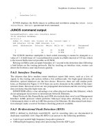
Now, assume that a remote router gets two conflicting messages at the same time. That
is, messages arrive almost at the same time claiming that a link is up and down. Consider
Figure 6.3. There are three routers connected by point-to-point links. Unfortunately, the
link between Router B and Router C is constantly going down, then up, and a short time
later, it goes down again. In network-speak this a flapping link. Next, assume that Router
B is a busy router with its CPU being loaded close to the ceiling. Therefore, Router B is
slower in processing the link-down/link-up events. In addition, the subsequent regener-
ation of its LSPs that report the link as down or up to other routers is slower.
Figure 6.4 shows the LSP messages from Router A’s perspective. Both Router B and
Router C find out first that there is a link-up event. However, Router C processes that event
far faster than the overloaded Router B. The trouble occurs as the link flaps again, this time
transitioning from the Up to the Down state. Router B still did not send the previous LSP
out because it was too busy. Router B’s LSP is now outdated information because the link
is now in the Down state. So both LSPs (Router B’s old Up one and Router C’s accurate
Down one) arrive at the same time at Router A. Now Router A needs to decide which is the
most accurate report – the Up or Down state message. The LSP to use should be the most
recent one, but in the example the most recent rule would fail because the propagation
delay from Router B to Router A made that inaccurate LSP arrive after Router C’s up-to-
date LSP. The conclusion here is that LSPs need to carry some sort of version information
to explicitly tell the receiving router what is current and what is outdated LSP information.
6.3.1 Sequence Numbers
Link-state routing protocols carry version information through a Sequence Numbers
field. IS-IS has a linear sequence number space starting from one and counting up. That
means that the first LSP that is announced by a router has the sequence number 0x1.
Each time the router issues a new view of the local environment to its neighbours, the
router will package that information in an LSP, increment the sequence number by one,
and send the LSP to all of its neighbours. The neighbours compare the incoming LSP
with the LSP in the local database. If the received LSP is new to them (that is, the

LSPs and Revision Control 147
What is the most recent
message?
Router A
Router B
Router C
FIGURE 6.3. The routers have to find out what is the most recent event
received LSP is not in the local database at all), then they unconditionally install the LSP
into their local link-state database. If the LSP is already installed in the database, the
receiving router needs to check if the sequence number is higher than the sequence num-
ber of the LSP that is already installed in the link-state database. If the LSP is newer, then
the router will flush (or discard) the existing LSP and update the LSP with the more
recent one. If it turns out (like in the previous example) that the most recent arriving LSP
is older (has a lower LSP sequence number) then the one installed in the link-state data-
base and therefore carries outdated information, the received LSP is silently discarded.
As IS-IS is a reliable protocol, the router will of course acknowledge receipt of that LSP
to the neighbour that sent it. If not acknowledged, the router will see the LSP again after
5 seconds, once the neighbour retransmits it. You can learn more about acknowledging
and retransmission of LSPs in Chapter 8.
The LSP sequence number field is a 32-bit identifier, giving room for about 4 billion
LSP updates. LSPs are subject to strict pacing, which means, for example, that a router
must not originate more than one LSP every 5 seconds. 2^32 times 5 seconds results in
an interval of 21,474,836,480 seconds, or roughly 681 years. So the sequence number
space is not likely to get to its end, at least not until readers are retired, which is typically
the timeframe that engineers care about.
Seriously, it is just assumed that the LSP sequence space will not run out. Assumptions
always cause a lot of trouble for engineers. The root-cause of the Y2K scare went back to
148 6. Generating, Flooding and Ageing LSPs
“slow”
Router B

Router C
t
tt
Router A
LSP
Router B
Link Up to Router C
Link “Up”
Link “Down”
Big
processing
delay
Big
processing
delay
LSP
Router B
Link Down to Router C
LSP
Link Up to Router C
Router C
LSP
Link Down to Router C
Router C
Little
processing
delay
Little
processing
delay

Conflicting
Messages
hit Router A
FIGURE 6.4. In distributed environments Router A can get confused if the Link-Up or Link-Down
is the most recent event
assumptions about events that should not be a problem but ultimately were. The bottom
line is the Y2K problem cost corporate customers a lot of money to sanity check their
applications and to spot software problems before the millennium turnover. But IS-IS is
well prepared in that respect, since there actually is something that can be done if the LSP
sequence number space is ever maxed out. So what does a router do if it wants to originate
a new LSP and does hit the ceiling of the LSP sequence space? Now, the assumption is
that this ceiling will never be reached. But even if it finally is, there is a well-defined pro-
cedure to handle that event: the router must simply wait for a period of max-age seconds.
This sounds odd at first: why does waiting solve anything? And how long does max-age
last? As it turns out, it lasts a Lifetime – an LSP’s Lifetime.
6.3.2 LSP Lifetimes
In addition to the revision information (the LSP sequence numbers), link-state protocols
include in their LSPs a field called the Lifetime, which helps to control the maximum
validity span of LSPs. A router announcing an LSP does not mean that the LSP will be
valid forever, only for the number of seconds indicated in the Lifetime field of an LSP.
Adding a Lifetime field to the protocol helps to protect against stale (and potentially
wrong) entries in the link-state database. Consider a scenario where a router is taken out
of the network by being powered down. The LSP(s) of that powered-down router is or are
still installed in the link-state database of all the routers in the network. If the originating
router did not revoke or purge them (you will see shortly how this works), the LSPs would
stay in the link-state database forever. The Lifetime field in the LSP is a 16-bit entity,
which means that the Lifetime field can be set as high as 2^16-1 or in decimal notation
65,535 seconds, or a little over 18 hours.
The Lifetime field provides an answer to the unlikely event of IS-IS LSP sequence num-
ber space exhaustion. Before an IS-IS router can generate a new LSP with a sequence

number of 1, the router must wait until the Lifetimes of all previous LSPs it has generated
has expired and the LSPs have disappeared from all other routers’ link-state databases.
At most, this wait (max-age) will be 18 hours. This sounds very high, but waiting 18 hours
every 681 years should not be much of a problem for a network. And in practice, IS-IS
implementations only use the maximum 18-hour Lifetime when extreme background
flooding silence is needed. Most of the time, IS-IS uses the default Lifetime value of
1200 seconds (20 minutes). This value can be changed in most IS-IS implementations,
and often it is changed. But what stops every LSP from disappearing from the network
every 20 minutes? A periodic LSP refresh.
6.3.3 Periodic Refreshes
LSPs with maximum Lifetimes have the consequence that LSPs need to get refreshed.
Refreshing means that a router has to re-originate its LSPs periodically. The re-origination
interval has, of course, to be less than the LSP’s Lifetime. For example, if the LSP is
valid for 1200 seconds (the default value), the router needs to refresh the LSP in less than
1200 seconds in order to avoid removal of the LSP from the link-state database by other
LSPs and Revision Control 149
routers. The recommended max-LSP-origination-interval is the Lifetime minus 300 sec-
onds. So in a default environment this would be 900 seconds.
Figure 6.5 shows in a timing diagram how and when a router refreshes its LSPs. Every
900 seconds an LSP with the same information content is created. Here, Router A always
reports that the router has links in the Up state to Router B and C. Please note that for
each refresh, the Sequence Number is incremented by one (bumped). Each time that LSP
is refreshed, the Lifetime gets prolonged for another N seconds, as described in the
Lifetime field (the default value is 1200 seconds).
Both Cisco IOS and JUNOS software do originate all LSPs with a default Lifetime of
1200 seconds, as suggested in the ISO 10589 specification. However, you can change
this to higher values to reduce the amount of refreshes in the network (the refresh timer
is seldom made a lower value). Often theses periodic LSP refreshes are called refresh
noise, and network administrators want to reduce this noise close to zero. Both Cisco
IOS and JUNOS software offer configuration knobs to change the maximum Lifetime of

their LSPs and at the same time the re-origination interval derived from this value. IOS
lets you define the Lifetime and refresh intervals independently from each other. All you
have to make sure of is that the max-lsp-lifetime be a few hundred seconds higher
than the lsp-refresh-interval. If you modify the max-lsp-lifetime do
not forget to set the lsp-refresh-interval accordingly (a few hundred seconds
lower than max-lsp-lifetime). If you forget to set the refresh interval, then the
LSPs will get refreshed according to the default timer, which is 900 seconds. This will
not break anything but it also does not help to reduce the refresh noise. The outcome
might be an LSP originated with the maximum Lifetime of 65,535 seconds which will
still be refreshed each 900 seconds.
In IOS you can set the LSPs Lifetime and refresh interval independently from each
other, as shown in the following (note the bolded sections in this code listing).
IOS configuration
In IOS the max-lsp-lifetime and lsp-refresh-interval parameters need to be at
least 300 s apart.
Amsterdam# show running-config
[… ]
router isis
max-lsp-lifetime 65535
lsp-refresh-interval 65000
[… ]
The JUNOS software only exposes the lsp-lifetime knob to the user interface.
The developers at Juniper Networks feared that inconsistent setting of Lifetime and
refresh interval might mess things up seriously. As an example, think about what might
happen if the Lifetime is set to be smaller than the refresh interval. The refresh interval
is calculated automatically. The refresh interval in a Juniper Networks router is the LSP
Lifetime minus 317 seconds.
150 6. Generating, Flooding and Ageing LSPs
151
LSP

Router A, Sequence 0x4
Lifetime 1200 s
LSP
Link Up to Router C
Link Up to Router B
Router A, Sequence 0x3
Lifetime 1200 s
LSP
Link Up to Router C
Link Up to Router B
Router A, Sequence 0x2
Lifetime 1200 s
1000
2000
3000
0
LSP
Link Up to Router C
Link Up to Router B
Router A, Sequence 0x1
Lifetime 1200 s
Periodic refreshes bump the Sequence Number every 900 seconds
t (s)
max LSP lifetime 1200 s
max LSP lifetime 1200 s
max LSP lifetime 1200 s
max LSP lifetime 1200 s
Link Up to Router C
Link Up to Router B
F

IGURE
6.5. Periodic refreshes
In the JUNOS software, the refresh interval is automatically calculated as the LSP refresh
interval equal to the Lifetime minus 317 seconds. In the following listing, the relevant
JUNOS software configuration is marked in bold:
JUNOS configuration
hannes@New-York> show configuration
[… ]
protocols {
isis {
lsp-lifetime 65535;
interface lo0.0;
interface so-0/0/0;
}
}
[… ]
As we can control how long an individual LSP will last (given that there is no change
in the network) we will unveil how an LSP actually looks and what particular informa-
tion it contains.
6.3.4 Link-state PDUs
Figure 6.6 shows the structure of a link-state PDU. In the common header, the Length
field is fixed to 27 bytes. The code points for the PDU type are 18 for Level 1 LSPs and
20 for Level 2 LSPs. The common LSP header contains the PDU length, which is the
aggregate length of the IS-IS PDU excluding Layer 2 information (such as PPP, Cisco-
HDLC, and MAC addresses). In the LSP header, the four most important elements are:
•
Lifetime
•
LSP-ID
•

Sequence Number
•
Checksum
The purpose of the Sequence Number and Lifetime fields was already discussed in the
previous sections. The 16-bit Checksum field contains an international standard X.233
Fletcher Checksum. The Fletcher Checksum is a simple checksum algorithm that, in add-
ition to protecting the payload of the LSP, ensures that there is no imbalance between zeros
and ones in the resulting checksum. Checksums generally help to make bit errors introduced
by WAN transmission more recognizable by the receiver. You can learn more about
checksums and what particular problems they solve in Chapter 13, which gives a good
overview of IS-IS checksumming, failure scenarios, and checksumming related defects.
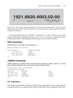
The LSP-ID field determines the LSP type. Figure 6.7 shows the structure of the LSP-
ID field. The LSP-ID is a fixed 8-byte field. The first 6 bytes are set to the System-ID of
the LSP Originator. The System-ID has the purpose of uniquely identifying a router in
the IS-IS network. If you are familiar with OSPF, the System-ID can best be compared
with the Router-ID. The only difference is that OSPF Router IDs are 32-bits (4 bytes)
152 6. Generating, Flooding and Ageing LSPs
and IS-IS System-IDs are 48-bits wide. The only required property is that the System-ID
has to be unique. Assignment of System-IDs, conversion schemes from OSPF-based IP
Router-ID to IS-IS System-IDs, and further information about IS-IS addressing can be
found in Chapter 4. The next byte in the LSP-ID field is called the Pseudonode-ID. The
principle of pseudonodes are not easy to explain in a paragraph – that is why it takes an
entire chapter to explain them. As a quick explanation, to an IS-IS router, a LAN consists
of real routers (nodes) and one router that represents the whole LAN but does not really
exist – the pseudonode. If the pseudonode byte is set to zero, we can be sure that this is
LSPs and Revision Control 153
Intra-domain Routing Protocol Discriminator
Header Length Indicator
Version/Protocol ID Extension
0x83

Bytes
1
1
1
1
1
1
1
1
1
ID Length
PDU Type
R
0
R
0
R
0
PDU Version
Reserved
Maximum Area Addresses
6 (0)
1
3 (0)
0
TLV section
0–1465
18, 20
27
Remaining Lifetime

LSP-ID
PDU Length
Sequence Number
2
2
ID Length (6) ϩ 2
4
Checksum
2
P
1
ATT ATT ATT ATT OL IS Type
FIGURE 6.6. The format of a link-state PDU
1921.6820.4003.02-00
System-ID
Pseudonode-
ID
Fragment-ID
FIGURE 6.7. The elements of a LSP-ID
a real router. If the pseudonode byte is non-zero then it represents the whole LAN . In
IS-IS LANs are represented in the link-state database with a unique identifier. More
information about pseudonodes and why they make sense is presented in Chapter 7.
The last byte in the LSP-ID field is called the Fragment ID. IS-IS runs directly on top
of OSI-RM Layer 2, which does not have a built-in fragmentation function for larger-
than-MTU-sized packets. IP-based routing protocols, such as OSPF, rely on IP to pro-
vide this fragmentation service, but IS-IS is not IP-based. So IS-IS needs to support
fragmentation through the application itself: IS-IS. Once again, IS-IS fragmentation is
worth a chapter on its own, because there are lots of interesting issues surrounding IS-IS
fragmentation such as “What should be done if a fragment of an LSP is missing”, “Is
there a special meaning to fragment zero”, and “What should be done if the fragment

space itself is exhausted?” Chapter 9 is dedicated to giving answers to these and other
questions surrounding fragmentation.
LSP-IDs are not displayed as a string of 8 consecutive bytes. In modern routing soft-
ware LSP-IDs follow certain conventions. In the next paragraphs the notation of LSP-
IDs will briefly be discussed. Furthermore we spot on more detailed what bits the
Attribute Type Block contains and what particular Application of the Overload Bit
may be.
6.3.4.1 LSP Notation
Typically the LSP-ID is displayed in the following format:
xxxx.xxxx.xxxx.yy-zz
Here, an x stands for the System-ID digits, y stands for the Pseudonode-ID, and z rep-
resents the fragment number. Let’s have a look at a tcpdump showing an LSP header and
its contents. The following shows a real-world LSP. Look especially at the notation used
for the LSP. The fields of the LSP header are shown in bold:
Tcpdump output
11:36:45.587565 OSI, IS-IS, length: 405
L2 LSP, hlen: 27, v: 1, pdu-v: 1, sys-id-len: 6 (0), max-area: 3 (0)
lsp-id: 1921.6800.0012.00-00, seq: 0x000002fd, lifetime: 1198s
chksum: 0xe984 (correct), PDU length: 405, Flags: [ L1L2 IS ]
Authentication TLV #10, length: 7
simple text password: !$xyz00
Area address(es) TLV #1, length: 4
Area address (3): 49.0001
Protocols supported TLV #129, length: 1
NLPID(s): IPv4 (0xcc)
Hostname TLV #137, length: 6
Hostname: London
IPv4 Interface address(es) TLV #132, length: 4
IPv4 interface address: 172.16.1.33
154 6. Generating, Flooding and Ageing LSPs

IPv4 Internal Reachability TLV #128, length: 84
IPv4 prefix: 10.254.47.8/30, Distribution: up, Metric: 5, Internal
IPv4 prefix: 10.252.1.0/30, Distribution: up, Metric: 5, Internal
IPv4 prefix: 10.254.1.48/30, Distribution: up, Metric: 1, Internal
IPv4 prefix: 10.254.1.20/30, Distribution: up, Metric: 5, Internal
IPv4 prefix: 10.254.3.4/30, Distribution: up, Metric: 25, Internal
IPv4 prefix: 10.254.1.72/30, Distribution: up, Metric: 2, Internal
IPv4 prefix: 10.254.1.28/30, Distribution: up, Metric: 5, Internal
Extended IS Reachability TLV #22, length: 75
IS Neighbor: 1921.6800.1001.00, Metric: 5, sub-TLVs present (64)
IPv4 interface address subTLV #6, length: 4, 10.154.1.6
IPv4 neighbor address subTLV #8, length: 4, 10.154.1.5
Unreserved bandwidth subTLV #11, length: 32
The first output of the second line shows us an LSP-ID. We recognize that this is an
LSP-ID because it follows the xxxx.xxxx.xxx.yy-zz style. Only LSP-IDs follow that
style. The last bold argument in the tcpdump output shows the so-called Attribute Type
Block, which has in the example two bits set.
6.3.4.2 Attribute Block
What are the Flags [ L1L2 IS] following the checksum? What are they used for? The last
byte in the LSP header is often referred to as the attribute block. These 8 bits tell the
receiver crucial information about the nature of the LSP. These 8 bits are:
•
Bit 8 – P (Partition Repair) Bit
•
Bit 7 – ATT-Error Bit
•
Bit 6 – ATT-Expense Bit
•
Bit 5 – ATT-Delay Bit
•

Bit 4 – ATT-Default Bit
•
Bit 3 – OL (Overload) Bit
•
Bit 2 and 1 – IS Type Bits
The P (Partition Repair) Bit is what is known as a capability indicator that shows if the
issuing router supports the partition repair functionality (that is, this bit indicates that
capability). Partition repair means that a broken Level 1 area can be healed through the
Level 2 IS-IS routers. It is not possible to be very specific here because Partition Repair
is barely deployed and sometimes even not supported in certain IS-IS implementations
such as JUNOS. Partition repair is left as an option to the implementer of the protocol,
so this is not a major issue. Typically, if a specification says that something is optional,
and if it is complicated to implement or does not solve a specific problem, this is enough
justification to ignore that function entirely. So if you take the time and crawl through
protocol specification, such as RFCs and Internet drafts or – even worse – ISO papers
and documents, then you almost always can replace the word “should” with “can-be-
ignored” in your mind.
LSPs and Revision Control 155
The next four bits in the Attribute block, Bits 7 to 4, determine if the issuing
Intermediate System is attached to another area or not. Only L1L2 routers may set this
bit in their Level-1 LSPs. But why are there 4 bits denoted to this functionality, and not
just one? Because at the time when ISO 10589 was specified (in the late 1980s) many
people believed that routing protocols should support multiple topology databases, each
set up for a particular purpose. The original idea was that IS-IS should calculate one
topology database that would have the lowest bit error rate, one topology database for
the least expensive paths in the network, one that reflects the lowest delay topology,
and finally one that would be used if the sender of the packet were undecided which
of the topologies to pick. This is an early form of Class-of-Service (CoS) enabled
routing, which ultimately did not get deployed because network engineers felt uncom-
fortable (rightly so at the time) about supporting such multidimensional networks. Bits

5, 6 and 7 therefore got deprecated (not quite obsolete, but not promoted at all) over time.
Today, as far as IP routing is concerned both JUNOS and IOS only support the default-
metric, and hence just the bit 4 default topology, which only demands a single instance
of SPF calculation. There are more places in the IS-IS specification where this
CoS-based routing legacy pops up; however, in modern routing it has been entirely
deprecated.
The Overload Bit is used (not surprisingly) to indicate that a router is in an overloaded
condition. Initially, this was envisioned to serve as an indicator that a router had run
out of memory. Running out of memory in a router is never good, but the impact of
memory shortage is especially dramatic for link-state protocols: if a router cannot store
all LSPs in its link-state database the router will not be able to calculate loop-free
paths through the network. The idea behind the Overload Bit is that once the router
notices that it is running short of memory, the router will simply refuse to play SPF with
neighbours and pull itself out of the game. A router holding half of the information
needed for proper SPF calculations, and disturbing the other routers by advertising
this half-knowledge does more harm than a router that reliably takes itself off the net-
work topology. The effect of a router originating its LSPs with the Overload Bit set
is that during the SPF calculation, the router will be disregarded for delivery of transit
traffic. The nice thing here is that the local sub-nets that the router still advertises in its
LSPs are still reachable. You can read more about the advertisement of IP sub-nets in
IS-IS in Chapter 12. So although the router is pruned from the network topology, the
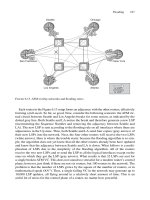
router is still reachable by non-transit packets. Figure 6.8 shows you the network impact
of a router that has the Overload Bit set. New York has the Overload Bit set in its
most recent LSP. Therefore, the routers in the network re-calculate their paths and
re-route around New York. For instance, Washington to Pennsauken traffic is moved
through the Frankfurt path. However, the local prefixes (and the loopback) IP address
of the New York router are still reachable. Local traffic therefore still goes directly to
New York.
The remaining two bits are the IS bits which indicate the topologies that the sender is in.
Each router is always in a Level-1 topology even if the router software lets turn you off

the Level-1 entirely off a Router. This is admitted a bit odd. So Bit 1 must always be set.
However, Bit 2 is variable. If it is set the router is also present in the Level 2 topology.
156 6. Generating, Flooding and Ageing LSPs
You can examine the contents of the Attribute block by issuing a show isis
database. This command is supported on both IOS and JUNOS routers, as shown in
the following:
IOS command output
Amsterdam# show isis database
[… ]
IS-IS Level-1 Link State Database:
LSPID LSP Seq Num LSP Checksum LSP Holdtime ATT/P/OL
LSPs and Revision Control 157
172.16.1/24
Pennsauken
LSP
New-York, Seq 0x2fc
Lifetime 1200 s, OL
Link Up to Pennsauken
Link Up to Wash D.C.
Pennsauken
Frankfurt
London
Washington
NewYork
Paris
FIGURE 6.8. The overloaded routers’ local prefixes are still reachable while transit-traffic is
kept away
New-York.00-00 0x00002fac 0xC24F 60128 1/0/0
[… ]
IS-IS Level-2 Link State Database:

LSPID LSP Seq Num LSP Checksum LSP Holdtime ATT/P/OL
LINX-gw.00-00 0x00000128 0xB8EF 36163 0/0/1
LINX-gw.01-00 0x00000128 0x455A 42001 0/0/0
VIX-gw.00-00 0x00000123 0xEFC1 5023 0/0/0
[… ]
In JUNOS, you can get a quick overview of the status of some of the bits by issuing
the show isis database command. If you want to see the Attribute block for
one LSP specifically, then you can request a specific LSP’s extensive output by
issuing a show isis <LSP> extensive. There are various levels of output for the
show isis database command. You can see the default and how the extensive
modifier changes the output in the following:
JUNOS command output
hannes@New-York> show isis database
IS-IS level 1 link-state database:
LSP ID Sequence Checksum Lifetime Attributes
New-York.00-00 0x2fac 0xc24f 62063 L1 Attached
[… ]
4 LSPs
IS-IS level 2 link-state database:
LSP ID Sequence Checksum Lifetime Attributes
LINX-gw.00-00 0x128 0xb8ef 36063 L1 L2 Overload
LINX-gw.01-00 0x128 0x455a 41901 L1 L2
VIX-gw.00-00 0x123 0xefc1 4922 L1 L2
[… ]
12 LSPs
hannes@New-York> show isis database LINX-gw extensive
LINX-gw.00-00 Sequence: 0x128, Checksum: 0xb8ef, Lifetime:
36063 secs
IS neighbor: London.01 Metric: 2000
IP prefix: 2.168.9.225/32 Metric: 0 Internal

IP prefix: 172.16.6.0/28 Metric: 2000 Internal
[… ]
Packet: LSP id: Vienna-ts1.00-00, Length: 98 bytes, Lifetime:
36063 secs
Checksum: 0xb8ef, Sequence: 0x128, Attributes: 0x7 <L1 L2 Overload>
NLPID: 0x83, Fixed length: 27 bytes, Version: 1, Sysid length: 0 bytes
Packet type: 20, Packet version: 1, Max area: 0
158 6. Generating, Flooding and Ageing LSPs
The use of the Overload Bit is one of the more interesting stories of IS-IS. The reason
why and when this bit is set has changed dramatically over the years. At first, the use was
straightforward: there were many router memory constraints. Memory in the late 1980s
compared to today was expensive, and the chips had little capacity. In the late 1980s,
most routers were running with 512 KB of memory. So memory was definitely a con-
straint, and the Overload Bit was used as intended.
But what about today? Memory isn’t really an issue for IS-IS now. All modern Internet
core routers have at least 256 MB of memory, and in many cases, they have even more
memory. For example, the Juniper Networks T640 router has a route-processor that has
a massive 2 GB for storing routing information. And IS-IS is not a particularly memory-
intensive protocol. Massive amounts of memory are typically needed for storing BGP
routes and paths. Even in the largest networks in the world, IS-IS does not consume more
than 1.5 to 2.0 MB of memory. To give an idea how big these modern IS-IS networks are,
think of an L1L2 router that is on the IS-IS Level 2 backbone with 1200 or more other
routers. In addition, consider 200 or more routers at IS-IS Level 1. Thus, the link-state
database is quite large. True enough, and yet it still does not consume more than between
0.1% and 1% of a modern route processor’s memory. So what is it that drives the setting
of the Overload Bit today? The answer to this is addressed in the next section.
6.3.4.3 Applications of the Overload Bit
In an Internet core router there are always two routing protocols running. One is for gather-
ing topological knowledge and one carries a bulk amount of reachability information.
The Interior Gateway Protocol (IGP) discovers the topological knowledge of the internal

core network of an ISP. IS-IS is a member of the large family of IGPs. For the reachabil-
ity information about bulk routes (Internet routes and customer routes), there is the
Border Gateway Protocol (BGP), the interdomain routing protocol of the Internet. Each
protocol does what it can do best. IS-IS quickly discovers, and then re-routes the internal
network. Unfortunately, IS-IS is not very good in transporting a bulk amount of routing
information across the internal network. IS-IS is in good company in being unsuited for
this task with the rest of the IGPs (RIP, OSPF, EIGRP etc.).
All of the IGPs suffer from the same protocol defect, in that all of the IGPs do not have
any flow-control mechanisms built into the protocol. This is the reason that they fail
when a large number of routes have to be carried across the internal network. As long as
the IGP routers are loaded moderately, there is not much of a problem. However, as with
human beings, everything is different under stress. Once the network is exposed to
protocol-related stress (a large amount of re-routing, heavy LSP processing, many flap-
ping links, and so on), plus a large amount of BGP reachability information, the network
starts to churn. Churning IGPs was the typical reason in the 1990s when people like the
NOC-team managers and the Chief Technology Officer got paged out of bed in the middle
of the night.
These lessons were learned and the implementations of the routing protocols did get
better. There has also been more experience gained in network design. The pragmatic
design rule today is that there must not be any other IP reachability information in the
LSPs and Revision Control 159
IGP other than /30, /31 (point-to-point link IP sub-nets) and /32 routes (loopback addresses).
No customer routes, no server farm routes, nothing except the IP sub-nets needed to run
the internal infrastructure is put into the IGP’s database. Common practice is that all of
the IP reachability information is injected into BGP, which, because BGP runs on top of
TCP, is very good in terms of flow-control. So if a BGP peer wants to throttle down a
neighbouring speaker that is too fast, the router simply delays the TCP acknowledgements.
Delayed TCP ACKs emulate a small bandwidth link. The fast speaker will back off and
reduce the pacing of the route transmission.
But if BGP is so good, then why do we need IGPs like IS-IS? To answer this, you have

to understand that there is some mutual dependency between the IGP and BGP. First of
all, BGP runs on top of TCP, and in order for TCP to work, you need valid internal routes
to get your BGP session up and running. Furthermore BGP needs some information
about how far a BGP speaker is away to determine the best route – it is the IGP that sup-
plies that information. On the downside BGP converges (produces consistent informa-
tion in all BGP routers) very slowly particularly because it is not very good in detecting
that a neighbour is down as it has very slow paced keep-alive timers. Once the BGP
neighbour is determined to be down in the worst case, it can take up to 2 minutes for a
BGP router to declare a neighbour down. IS-IS is much quicker (orders of 10–30 sec-
onds) to detect absent peers. It is the slowness of BGP, more precisely the slowness of
iBGP (BGP distributing information to the internal network), that mandates the use the
Overload Bit today.
Consider the scenario shown in Figure 6.9. It shows a transit provider providing ser-
vice to the customer ASs 2 and 3. The iBGP connections as they should be in the
converged state are represented in the diagram as dotted curves. However, the internal
BGP sessions to Core Router #2 are down because we had to reboot Core Router #2 (the
reason for this reboot is unimportant, but happens occasionally). The router reboots,
starts its routing processes (IS-IS and BGP), and tries to get the iBGP sessions up, but it
can’t! This is because IS-IS has not yet learned about the internal topology to acquire the
necessary routing information in order to get the internal BGP sessions, which rely on
TCP, up. IS-IS starts to discover its directly connected neighbours (Core Router #1, #3,
Border Router A, B) and starts to synchronize its link-state databases. Database synchro-
nization is discussed in more detail in Chapter 8.
After database synchronization, the IS-IS routing process schedules an SPF calcula-
tion and feeds the routing information resulting from that calculation into its local
routing table. This is the beginning of the black hole state where packets flowing into a
router have no place to go. Border Routers A and B immediately send Core Router
#2 traffic targeted to local AS 2 and 3. The problem is that Core Router #2 does not
yet have the transit BGP routes to know where to forward that traffic, as the iBGP
sessions are not established yet. After a while, the sessions to the iBGP speakers are

established (this can last up to several minutes) and Core Router #2 will have built up
accurate forwarding states to pass on the traffic and so as not to black hole the packets
any longer.
What can be done in IS-IS to help avoid entering a black-hole scenario? Consider what
would happen if Core Router #2 sets the Overload Bit when sending its first LSP. During
the subsequent SPF calculation, the Border Routers A and B will detect the Overload Bit
160 6. Generating, Flooding and Ageing LSPs
during processing Core Router #2’s LSP and will therefore eliminate Core Router #2 as
a possible way to send transit traffic. The transit traffic will be routed around Core Router
#2 over Core Routers #1 and #3. The good news is that Core Router #2’s local sub-nets
will still be reachable even if the router sets the Overload Bit, so the iBGP sessions to all
the internal routers can be established successfully during the overload condition.
Most IS-IS implementations, including IOS and JUNOS software, support static set-
ting of the Overload Bit. The following configuration statements show how to set the
Overload Bit statically. The set-overload-bit command sets the Overload Bit for
both levels of the IS-IS instance, as shown in the following:
IOS configuration
The IOS set-overload-bit command sets the Overload Bit persistent static and does
not remove it after some time.
Amsterdam# show running-config
[… ]
router isis
set-overload-bit
[… ]
LSPs and Revision Control 161
FIGURE 6.9. IS-IS and BGP routing is mutually dependent on each other; if both do not converge at
the same time, traffic is black holed
140K Internet
Routes
Core Router #1

Core Router #3
Border Router B
Border Router A
Core Router #2
iBGP
eBGP
140K Internet
Routes