The Complete IS-IS Routing Protocol- P28 potx

10.3.1 Full SPF Run
The full SPF run is the heavyweight of SPF flavours. It both re-computes the topological
grid in an area as well as re-computes the reachable IP prefixes. Full SPF runs are typi-
cally triggered by the following events:
•
Local configuration change
•
Update to a known LSP, which contains an adjacency change
•
Local aged adjacency
•
Receipt of a new/unknown LSP
•
New Area-ID in the Level-1 network
•
Link metric change
•
Purging an LSP
•
Periodically for additional robustness (every 15 minutes)
The full SPF run is not scheduled immediately after the above trigger events. Instead it is
delayed for a configurable minimum amount of time. The most typical event from the
above list is a new or updated LSP. In IS-IS networks, as in any other network running
link-state routing protocols, there is a general observation that single LSP updates are
very rare. They are almost always accompanied by other LSPs, which follow shortly
after the first LSP shows up. The reason behind this is very clear: if a link fails there are
always two routers that need to re-originate their LSPs. So it is better to wait a couple of
milliseconds before starting an SPF calculation, which may tie the router down on the
order of 100s of milliseconds.
So routers delay the SPF calculation. The typical pre-SPF delay value is 100 or 200 ms
(depending on IOS or JUNOS). After the pre-SPF delay, the router freezes the link-state

database and does the SPF calculation. Freezing means that during this time, no LSP
additions or changes can be made.
10.3.1.1 Link-state Database Locking
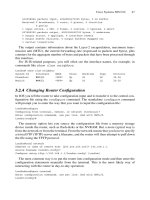
It is absolutely mandatory for an IS-IS implementation to freeze the database during an
SPF calculation run. An LSP change inserted during a run of the SPF calculation may
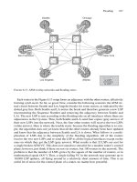
result in bogus routes. Consider Figure 10.10 to get an idea what will happen if the link-
state database is not locked. We are in the middle of an SPF calculation. The early stages
of the SPF calculation considered the path through Washington the best path in the network.
Now it is exploring the network downstream from Washington. Suddenly, the link between
Washington and New York goes down. Unfortunately, the New York–Washington path is
our best-path candidate. The SPF calculation does not backtrack through path candidates
to see if the path properties have changed. If the router does not lock the link-state database
then the result will be most likely bogus routes. Of course, IOS and JUNOS both lock the
database (as any serious IS-IS implementation has to) and queue any incoming LSPs for
insertion once the database is unlocked.
After the SPF calculation has completed, the router starts an SPF hold-down timer
which blocks further SPF runs for self-protection reasons.
258 10. SPF and Route Calculation
SPF Calculation Diversity 259
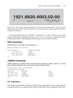
10.3.1.2 Self-protection
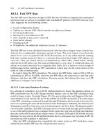
The purpose of hold-downs is to allow the IS-IS router to work less. Consider Figure 10.11
to see why SPF hold downs make sense. If there were no hold-down for SPF calculation,
then the average utilization of the control plane CPU would be very high. During an SPF
calculation (100–200 ms) the CPU utilization jumps to 100 per cent. But shortly there-
after it drops down to 0 per cent. If a network is shaky, then additional LSPs triggering
new SPF calculations will follow, raising the CPU utilization to 100 per cent once again
for a short period of time. By applying SPF hold-down timers, IS-IS keeps the intervals
between the SPF calculations large and so lowers the average CPU utilization spent for
SPF calculations. In other words, SPF hold-down is a self-protection mechanism to avoid
meltdown of the router’s control plane. SPF hold downs trade responsiveness for stability.

What is gained is a router control plane that is stable in every situation and does not go
down the “CPU churning spiral” when the network starts to get shaky. However, on the
other hand, a router loses responsiveness. Consider a router that is in the middle of an
87000600000
250000
22000 22000
315000
31500026000
London-ϾFrankfurt 22000
Frankfurt-ϾLondon 22000
Frankfurt-ϾParis 87000
Paris-ϾFrankfurt 87000
LSDB entry cost
315000Pennsauken-ϾLondon 315000
Washington D.C ϾParis 600000 648000
26000
via
Washington D.C 48000
298000
Pennsauken
oc192/STM-64 oc48/STM-16
New York
New York
oc48/STM-16
London
oc768/STM-256
Area 49.0001
Level 2-only
oc768/STM-256
Washington

oc192/STM-64
Frankfurt
oc12/STM-4
oc192/STM-64
Paris
UNKNOWN List
TENTative List
cost to root
Destination
New York New York
New York
New York
cost to root
Frankfurt
PATH List
FIGURE 10.10. If the contents of the LSDB are not locked during the SPF computation, bogus
routes will result
260
average utilization
15
20
25
t (s)
0
5 s hold down
20
40
100
CPU load [%]
5 s hold down

5 s hold down
5 s hold down
5 s hold down
60
80
5
10
Peak utilization
Peak utilization
Peak utilization
Peak utilization
Peak utilization
Peak utilization
F
IGURE
10.11. SPF hold-downs smooth the CPU utilization
SPF hold-down period: even if plenty of LSPs do rush in, the router has to wait until the
hold down period is over before scheduling the SPF calculation again. Then there are
considerations like “How short should the hold-down time be to still be responsive?” and
“How long should the hold-timer be to be stable enough?” and even “What is the optimal
hold-down timer value?”
Unfortunately there is no universal hold-down timer value that applies to all networking
scenarios. Hold-down timers are always a compromise between stability and responsive-
ness. Look at stability to start with: this mostly depends on network size and link stabil-
ity. Network engineers used to say “In a quiet environment, OSPF and IS-IS are quiet
protocols”.
In the infancy of link-state routing protocols there was usually a static SPF hold-down
timer of 5 seconds between SPF runs. This was a conservative timer, the better to scale
for large networks. Today, adaptive timers, which take into account the churn in the network,
are more common. The basic idea behind the new schemes is that the first couple of SPF

calculations are scheduled immediately without any notable delay and only subsequent,
persistent SPF runs are delayed. The more SPF runs need to be scheduled, the longer the
hold-down timer gets. Such schemes are a much better compromise between responsiveness
and stability than static timers can ever be.
The typical adaptive timer algorithm implementation reacts very fast, and is very
responsive at first. This covers 99 per cent of the typical network-changing events, which
are link failures. That means that two LSPs arrive within a very short window. For the
remaining 1 per cent of failure scenarios, the algorithm falls back to the older SPF hold-
down static intervals for self-protection reasons.
JUNOS and IOS have different ways of implementing hold-down timers. IOS imple-
ments a technique called exponential back off. Here the hold-down interval gets doubled
each time an SPF calculation is executed. The initial delay, the max-delay and the mini-
mum hold-down interval can be configured using the using the spf-interval
<max-holddown> [<initial-wait> <minimum-holddown>] configura-
tion command. The following shows a custom configuration of the SPF hold down
behaviour in IOS. This works as follows:
IOS configuration
In IOS there are three timers to control SPF hold-down. The first timer specifies the SPF
hold-down in the slower phase expressed in units of seconds. The second timer specifies
how many milliseconds to wait before scheduling the very first SPF calculation. The third
timer specifies the minimum SPF hold-down in the fast phase. The last two timers are
expressed in units of milliseconds.
London# show running-config
[… ]
router isis
spf-interval 5 200 1000
[… ]
SPF Calculation Diversity 261
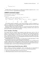
Figure 10.12 shows the timing behaviour of the exponential back-off algorithm compared
to the JUNOS style, called a “3 ϫ fast back-off” method. In IOS, the first SPF run is

delayed for 200 ms. Next, the minimum-hold-down timer kicks in, so scheduling of the
second SPF run will take at least 1000 ms as specified in the third argument of the spf-
interval configuration command. All subsequent SPF runs will get delayed for double
the previous hold-down time, 2 seconds for the third SPF run, 4 seconds for the fourth
SPF run, and so on. Similarly, the LSP origination interval, which was explained in
Chapter 6, “Generating, Flooding and Ageing LSPs”, also has a precaution that the hold-
down does not grow to infinite value. Clipping of the hold-down timer is done with the
first argument (5 seconds) of the spf-interval command. During every fast-build,
the SPF interval gets bigger until it hits the ceiling of 5 seconds. After a particular router
has not scheduled an SPF run for 20 seconds, the SPF hold-down state will be reset. This
means that from here on, any further SPF calculations will be scheduled “fast”, like the
first couple of SPF runs.
JUNOS takes a different approach. Instead of gradually getting slower, there is a fixed
number of fast runs, and after that the router falls back into slow scheduling mode. The
engineers at Juniper Networks argue that this linear form of back off has worked fine for
the past 10 years, and more sophisticated methods are not needed. In most implementations,
the static SPF hold-down period is set to 5 seconds and by straight switching between the
two modes, fast and slow, no harm is done.
JUNOS has an initial pre-SPF timer that defaults to 200 ms. It can be changed using
the spf-delay configuration command, which is available under the protocols
isis stanza. This command affects both the partial and the full SPF calculation and can
be changed in the range from 50 ms to 1000 ms.
JUNOS configuration
In JUNOS there is only one timer that controls SPF scheduling. The spf-interval con-
figuration command determines in units of milliseconds the initial-wait and inter-SPF wait
period when scheduling SPF calculations.
hannes@Vienna> show configuration
[… ]
protocols {
isis {

spf-delay 100;
interface lo0.0;
interface so-0/0/0;
}
}
All other values are hard coded into JUNOS. The number of fast runs is 3 and the min-
imum pre-SPF timer can go as low as 50 ms. In the above configuration example, the
router has to wait 100 ms before an SPF calculation is scheduled, and 100 ms between
SPF calculations.
262 10. SPF and Route Calculation
263
2000
4000
6000
8000
10000
12000
0
27000
5000 ms
hold down (max hold down)
After 20 s fallback to fast behaviour
IOS exponential hold-down behaviour
2000
4000
6000
8000
10000
12000
0

24000
After 20s fallback to fast behaviour
JUNOS (3x short, after that long) hold-down behaviour
First
LSP
rcvd
Second
LSP
rcvd
First
SPF
run
Second
SPF
run
Third
LSP
rcvd
Third
SPF
run
Fourth
LSP
rcvd
Fourth
SPF
run
1000 ms
hold down
2000 ms

hold down
4000 ms
hold down
t (ms)
t (ms)
First
LSP
rcvd
Second
LSP
rcvd
Third
LSP
rcvd
First
SPF
run
Second
SPF
run
Third
SPF
run
1000 ms
hold down
1000 ms
hold down
1000 ms
hold down
5000 ms

hold down (max hold down)
F
IGURE
10.12. IOS makes the hold-down interval exponentially longer – JUNOS starts with three short and after that uses long hold-do
wn intervals
10.3.1.3 Timer Compatibility Issues
It is recommended to keep at least the initial-wait timer the same across the IOS and
JUNOS routers in a network. Once they are the same it is certain that the SPF calculations
start and finish almost simultaneously. Due to the hop-by-hop routing paradigm, near
simultaneous SPF calculations and re-routing is desired to avoid transient loops. However,
it can never be guaranteed that two routers converge at the same time, but keeping the
timers current is usually good enough, or at least does not break the desired global conver-
gence intentionally.
The following two IOS and JUNOS configuration files are a good tradeoff between the
two schemes and have proven to work well even in large multi-vendor networks.
JUNOS configuration
An SPF delay of 100 ms means that the SPF algorithm converges fast and still provides
reasonable protection. The typical SPF run in large networks does not last longer than
100 ms. This 100 ms of quiet takes the average utilization down to 50 per cent.
hannes@Vienna> show configuration
[… ]
protocols {
isis {
spf-delay 100;
interface lo0.0;
interface so-0/0/0;
}
}
IOS configuration
The two 100 ms arguments make the initial-wait and minimum hold-down behaviour

exactly like JUNOS. The first argument specifies the maximum SPF hold-down value,
which is hard-coded in JUNOS as well.
London# show running-config
[… ]
router isis
spf-interval 5 100 100
[… ]
10.3.1.4 Performance and CPU Usage
The CPU cost of a plain, un-optimized SPF run is probably one of the most well-examined
algorithms in computer science. Before assessing worst-case figures, first consider two
factors: how many routers and how many links are in the network. Let the number of
routers be N and the number of links be L.
264 10. SPF and Route Calculation
SPF Calculation Diversity 265
It is actually very hard to predict the SPF runtime, as it is highly dependent on the
topology, that is, how the routers are meshed to each other. It has been shown above that
the tracking of nodes on the PATH list consumes the most cycles. So what is done is to
present a worst-case and an average-case scenario, considering the number of routers (N)
or the number of links (L). To find out what the real SPF runtime will be, and it will be
somewhere between the two figures, how densely meshed the network is has to be taken
into account.
For a router-based, worst case estimate, simply take a look at the number of routers
and the number of search operations, assuming that every router is in the worst case con-
nected to every other router (a full mesh). Therefore, for a total of N nodes, at maximum
N–1 iterations steps are needed for the search operation to find out if the actual path is
better than the TENTative path. This is quite intuitive. Mathematically speaking, the runtime
requirements of the SPF run equals N
*
N–1 or O(N^2). Squared growth is really, really
the worst case.

Exploring all the feasible path scales directly, along with the absolute number of links
it can be shown that the SPF computation time is proportional to the number of links in
the network. Mathematically speaking, O(L
*
log(L)).
For example, let the number of routers be 100 and the numbers of links be 400. Then
the worst-case estimate would be that O(N^2) CPU-time-units (100
*
100 ϭ 10000) are
spent. The abstract unit “CPU-time units” is used because such observations only make
sense in a comparative way. If there is a given number of nodes and a given number of
links in a network, and the current SPF run time, a good estimate of the CPU runtime in
the future, when the number of routers and the number of links is higher, can be made.
The pure link-based observation results in a computational complexity of L
*
log(L),
which is 400
*
(log(400)) ϭ 1040 of CPU time-units.
So there is a factor of 10 deviation between the two estimates. In reality both the number
of links and the number of routers need to be considered. Both figures are needed for the
meshing factor, that is, how densely a given set of routers is meshed. It will be shown
shortly that the link-based model is a much better approximation than the worst-case
estimate.
The model where the total SPF runtime equals N (log(N)*2*log(L)) turns out to work
best in practice. In this formula, both the number of links and the number of nodes plus
a factor of two go into the formula. The factor of two is needed because the two-way
check is part of the path selection algorithm. Based on that formula, the resulting calcula-
tions come very close to reality. See Table 10.1 for the best model of route-processor
CPU prediction around today.

The theoretical model was verified using a lab test based on two common route
processors: the Juniper Networks RE 3.0 taken from the M & T-Series of Routers, and
the GRP Routing Engine taking from the Cisco GSR 12000 series. The two route processors
were exercised using the Agilent QA Robot Router Control-Plane Stress Testing Software.
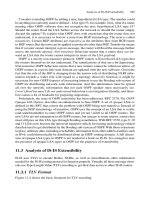
The Router Tester produces a grid, as shown in Figure 10.13.
Every 25 seconds, one link of the virtual topology was changed and the SPF runtimes
have been recorded using the show isis spf-log operational level CLI command
on IOS and show isis spf log on JUNOS.
IOS command output
London#show isis spf-log
Level 1 SPF log
When Duration Nodes Count Last trigger LSP Triggers
04:17:46 0.021189 408 1 virtual-5-3.00-00 DELADJ
TLVCODE
04:15:46 0.021224 408 1 PERIODIC
04:00:46 0.021712 408 1 PERIODIC
03:45:46 0.021323 408 1 PERIODIC
[… ]
JUNOS command output
hannes@Frankfurt> show isis spf log
IS-IS level 1 SPF log:
Start time Elapsed (secs) Count Reason
Sat Nov 1 15:04:34 0.017179 1 Periodic SPF
Sat Nov 1 15:19:03 0.017067 1 Periodic PF
Sat Nov 1 15:31:47 0.017081 1 Periodic SPF
Sat Nov 1 15:44:19 0.017334 1 Periodic SPF
[… ]
Sat Nov 1 15:45:07 0.017365 1 Updated LSP
[… ] virtual-5-3.00-00
Both outputs show the reason (trigger) and the duration of the SPF calculation.

The disparity between the theoretical prediction model and the simulation on the virtual
topology has been less than 3 per cent. Therefore, the model gives a good prediction of how
long the full SPF run will last in practice. The result of the simulation and the prediction
266 10. SPF and Route Calculation
TABLE
10.1. A prediction of real-world SPF runtime on common control plane CPUs.
Routers Links SPF runtime (ms) Juniper SPF runtime (ms) Cisco
Networks Routing Engine 3.0 Systems GRP 12000
100 250 1,92 4,80
200 500 4,97 12,42
400 1000 12,49 31,22
600 1500 21,18 52,94
800 2000 30,67 76,67
1000 2500 40,78 101,94
1500 3750 68,11 170,27
2000 5000 97,68 244,21
2500 6250 128,98 322,45
3000 7500 161,69 404,22
4000 10000 230,53 576,33
5000 12500 303,09 757,72
6000 15000 378,67 946,67
7000 17500 456,82 1142,04
8000 20000 537,19 1342,98
9000 22500 619,55 1548,86
10000 25000 703,67 1759,18
model are quite surprising. For even moderate to large topologies, the SPF calculation is
quickly finished after several tens of milliseconds. There are barely 30 IS-IS networks in
the world that have more than 400 routers and an SPF runtime greater than 50 ms
for their Level-2 routers. So for the majority of networks, SPF-runtime is an absolute
non-issue. It is certainly not the SPF runtime for the full SPF run that consumes a lot of

CPU resources.
10.3.2 Partial SPF Run
A partial SPF run only does recalculation leaf-related information. Partial runs are typically
triggered by the following events:
•
Metric of prefixes change
•
New prefixes
•
Deletion of prefixes
The partial SPF run is basically an extraction of all the prefixes in the link-state data-
base plus some information about the proximity of the prefixes (in simple words, a
SPF Calculation Diversity 267
SUT
F
IGURE 10.13. The SUT is exposed to a 7 ϫ 7 virtual grid to test SPF calculation time